Estimating aerodynamic roughness over complex surface terrain

Estimating aerodynamic roughness over complex surface terrain

Joanna M. Nield,1James King,2Giles F. S. Wiggs,2Julian Leyland,1Robert G. Bryant,3 Richard C. Chiverrell,4Stephen E. Darby,1Frank D. Eckardt,5David S. G. Thomas,2,5,6 Larisa H. Vircavs,1and Richard Washington2

Received 26 July 2013; revised 7 November 2013; accepted 11 November 2013; published 9 December 2013.

[1] Surface roughness plays a key role in determining aerodynamic roughness length (zo) and shear velocity, both of which are fundamental for determining wind erosion threshold and potential. Whilezocan be quantified from wind measurements, large proportions of wind erosion prone surfaces remain too remote for this to be a viable approach. Alternative approaches therefore seek to relatezoto morphological roughness metrics. However, dust-emitting landscapes typically consist of complex small-scale surface roughness patterns and few metrics exist for these surfaces which can be used to predictzofor modeling wind erosion potential. In this study terrestrial laser scanning was used to characterize the roughness of typical dust-emitting surfaces (playa and sandar) where element protrusion heights ranged from 1 to 199 mm, over which vertical wind velocity profiles were collected to enable estimation ofzo. Our data suggest that, although a reasonable relationship (R2>0.79) is apparent between 3-D roughness density andzo, the spacing of morphological elements is far less powerful in explaining variations inzothan metrics based on surface roughness height (R2>0.92). Thisfinding is in juxtaposition to wind erosion models that assume the spacing of larger-scale isolated roughness elements is most important in determiningzo. Rather, our data show that any metric based on element protrusion height has a higher likelihood of successfully predictingzo. Thisfinding has important implications for the development of wind erosion and dust emission models that seek to predict the efficiency of aeolian processes in remote terrestrial and planetary environments.

Citation: Nield, J. M., et al. (2014), Estimating aerodynamic roughness over complex surface terrain,J. Geophys. Res.

Atmos.,118, 12,948–12,961, doi:10.1002/2013JD020632.

1. Introduction

[2] The ability to quantify the momentum transfer between fluid flow and small-scale roughness elements is important in a myriad of environmental contexts including wind ero-sion and sediment entrainment schemes [e.g.Lettau, 1969;

MacKinnon et al., 2004; Lancaster, 2004;Lancaster et al., 2010], energy balance modeling [e.g. Brock et al., 2006;

Manes et al., 2008], and urban heat exchange [Oke, 1987]. This momentum transfer is parameterized by aerodynamic roughness,zo, and is a function of surface roughness,k, and

the arrangement and size of roughness elements [Raupach et al., 1991]. While vertical wind velocity profile or shear stress measurements can be used to measure zo directly

[King et al., 2008], there are many instances where only measurements of surface roughness (k) are available [Greeley et al., 1997]. Relationships between k to zo are

therefore required [MacKinnon et al., 2004], particularly for small-scale (sub-cm) roughness patterns, which to date have been little studied [Manes et al., 2008] and present additional challenges due to their continuous and complex morphologies [Marticorena et al., 2006]. Aerodynamic roughness over larger patterns is generally parameterized through investigations of discrete roughness elements at a wide range of spatial scales from small-scale wind tunnel studies [Brown et al., 2008;Cheng et al., 2007;King et al., 2008], medium-scale vegetation, and nebkha dune elements [Gillies et al., 2007;King et al., 2006;Lancaster and Baas, 1998; Marticorena and Bergametti, 1995; Raupach, 1992;

Raupach et al., 1993; Wolfe and Nickling, 1993] to large-scale building roughness elements of major cities [Castro et al., 2006;Grimmond and Oke, 1999;Millward-Hopkins et al., 2011;Rotach, 1995;Zaki et al., 2011] and remote sens-ing investigations [Blumberg and Greeley, 1993; Laurent

The copyright line for this article was changed on 23 OCT 2014 after original online publication.

1_{Geography and Environment, University of Southampton, Southampton,} UK.

2_{School of Geography and the Environment, Oxford University Centre} for the Environment, University of Oxford, Oxford, UK.

3_{Department of Geography, University of Sheffield, Sheffield, UK.} 4

School of Environmental Sciences, University of Liverpool, Liverpool, UK. 5_{Department of Environmental and Geographical Science, University of} Cape Town, Cape Town, South Africa.

6_{School of Geography, Archaeology and Environmental Studies,} University of the Witwatersrand, Johannesburg, South Africa.

Corresponding author: J. M. Nield, Geography and Environment, University of Southampton, Highfield, Southampton, SO17 1BJ, UK. ([email protected])

©2013. The Authors.

This is an open access article under the terms of the Creative Commons Attribution License, which permits use, distribution and reproduction in any medium, provided the original work is properly cited.

et al., 2005;Prigent et al., 2005]. In wind tunnel studies that assessed element configuration Cheng et al. [2007] and

Brown et al. [2008] found that the roughness element den-sity, rather than configuration, had the greatest influence on shear stress partitioning. Most aeolian transportfield studies only consider discrete roughness elements such as vegeta-tion, but the performance of sediment entrainment schemes for surfaces with continuous microroughness is less well quantified [MacKinnon et al., 2004] or parameterized using grain size [Darmenova et al., 2009]. Playas (or salt pans [Shaw and Bryant, 2011]) and small-scale rocky terrain surfaces (e.g., desert stony surfaces [Bullard et al., 2011] and sandar [Prospero et al., 2012]) typically comprise crusts or rock patterns of connected roughness elements at different scales. Although these elements are shorter than more commonly studied vegetation elements [e.g., Eamer and Walker, 2010;Brown and Hugenholtz, 2011;Weligepolage et al., 2012;Paul-Limoges et al., 2013], they still have the potential to significantly alterzoand the threshold wind stress

for sediment transport [Wiggs and Holmes, 2011]. These complex, rough, continuous surfaces present additional challenges for measurement and turbulence characterization, such thatfield studies to date have generally only undertaken transect measurements to characterize their roughness [e.g.,

Lettau, 1969;Lyles and Allison, 1979;Greeley et al., 1995;

Lancaster, 2004; Brock et al., 2006]. However, with the development of new technologies such as terrestrial laser scanning (TLS), the opportunity now exists to characterize surface roughness metrics in high resolution (mm scale) and in 3-D. These data sets can provide vital estimations ofzoin

areas where measuring aerodynamic profiles are infeasible but shear stress and erosion potential calculations are essential. [3] TLS is a technique whereby spatial coordinates of a

surface are measured remotely in a short time (minutes) over a moderate area (tens of square meters), thus enabling quan-tification of surface roughness at sub-cm scale [Buckley et al., 2008]. TLS has been used in a range of environments to spe-cifically measure small-scale surface roughness including (i) sand and soils [Eitel et al., 2011;Haubrock et al., 2009;Nield et al., 2011; Nield and Wiggs, 2011; Rodriguez-Caballero et al., 2012;Sankey et al., 2010;Smith et al., 2011], (ii) veg-etation [Anderson et al., 2010; Antonarakis et al., 2009;

Weligepolage et al., 2012], (iii) snow and ice [Kaasalainen et al., 2011;Nield et al., 2013;Wirz et al., 2011], and (iv) rocks [Fardin et al., 2004; Khoshelham et al., 2011] and has shown promise in relating these patterns to aerodynamic roughness [Hugenholtz et al., 2013]. Here we apply TLS to elucidate pattern variability over a broad range of roughness element sizes and pattern distributions associated with 20 typical playa and sandar dust-emitting surfaces [Mahowald et al., 2003;

Prospero et al., 2012]. We relate the quantified morphological characteristics (flat to cobble) to velocity profile-determined aerodynamic roughness (zo) values and provide a continuum

of predictive measurements for relatively smooth, complex patterns that are typically prone to wind erosion.

2. Background: Quantifying Surface Roughness

[4] The availability of accurate, high-resolution DEMs

derived from TLS surveys opens up the possibility of using a myriad of different terrain analysis techniques to quantify surface roughness magnitude and variation in one, two, or

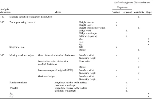
three dimensions. Conceptually, these different methodolo-gies define the magnitude of the surface elements’ height and spacing, or the variability of the surface patterning, as indicated in Table 1.

2.1. One-Dimensional Methods

[5] The simplest methods for characterizing surfaces

con-sider the height distribution of the surface, where the maxi-mum and standard deviation of height are taken to indicate element magnitude and roughness (surface variability), respectively [Glenn et al., 2006]. These nonspatially explicit metrics are commonly used as a measure of surface rough-ness in the analysis of complex large-scale building city-scapes or forested terrain [Nakayama et al., 2011].

2.2. Two-Dimensional Methods

[6] Two-dimensional (2-D) methods that characterize the

spatial aspects of surface roughness have traditionally been undertaken using transects of varying length. For example, in glacial researchMunro[1989] adapted theLettau[1969] method (LM) to characterize complex ice roughness. This LM method is calculated using equations (1–3) from

Munro[1989] and has been compared to aerodynamic mea-surements made by a number of researchers (e.g., Brock et al. [2006]). In the LM method transect lines are detrended and centered over a zero mean. The zero-up-crossing method [Goda, 2000] can then be used to calculate how many times the zero line is crossed in an upward direction through the transect line to give the frequency of continuous groups of positive height deviations:

kLM¼0:5h s

S (1)

s¼h

_X

2f (2)

S¼ X f

2

(3)

where kLM is the geometric roughness length equivalent

of measured aerodynamic roughness using the LM method,

h* is the average obstacle height (twice the standard devia-tion of the detrended elevadevia-tion in equadevia-tion (2)),sis the sil-houette area,Sis the unit ground area,Xis the length of the transect, andfis the roughness element frequency (number of continuous groups of positive height deviations above the mean elevation—calculated using the zero-up-crossing method in this instance).

[7] The zero-up-crossing method enables wavelength and

heights for each element to be calculated along a transect. The converse zero-down-crossing method can be used to de-termine when the zero line is crossed in a downward direc-tion, and the difference between neighboring up and down crossing pairs determines the ridge width and the distance between down and up pairs defines the interridge spacing (Sp). While discrete elements are generally assumed to be

(λ2-D) can then be specified from equation (4), assuming a

rectangular element cross section.

λ2-D¼ b1h1 L2L1

(4)

whereb1is the element width perpendicular to the wind

di-rection,h1is the element height,L1is the element wavelength

perpendicular to the wind direction, and L2 is the element

wavelength parallel to the wind direction.

[8] Similarly, a basal to frontal area ratio (RBF) can be

calculated using equation (5).

RBF¼ L2b1 h1b1

(5)

[9] Variograms are used in a range of continuous surface

roughness studies to assess pattern scaling, including in gravel river beds [Hodge et al., 2009;Huang and Wang, 2012], soil

[Croft et al., 2012, 2013;Sankey et al., 2012], and snow sur-faces [Schirmer and Lehning, 2011]. Commonly derived values include the sill, which is the value of semi-variance (y) at which convergence occurs and indicates roughness within the data, and the range, which is the corresponding lag distance (x) at convergence and indicates the point at which surface structures are no longer related.

2.3. Three-Dimensional Methods

[10] Three-dimensional (3-D) methods capture the full spatial

variability of the surface either locally via moving windows, or globally via complete surface analysis. Similar to the 2-D method, the standard deviation of elevations can be measured spatially by quantifying the convergent standard deviation value within moving windows of increasing size [Frankel and Dolan, 2007], as has been used in a variety of applications including bi-ological crust roughness [Rodriguez-Caballero et al., 2012].

Figure 1. Examples of (a) irregular salt pan, (b) regular, polygonal salt pan, and (c) sandur surface

patterns measured using the TLS.

Table 1. Classification of Different Physical Surface Roughness Metrics in Terms of Pattern Variability, Shape, and Magnitude

Analysis

dimension Metric

Surface Roughness Characterization

Magnitude

Variability Shape Vertical Horizontal

1-D Standard deviation of elevation distribution x

2-D Zero-up-crossing transects Height (mean) x

Height (max) x

Height (standard deviation) x

Ridge width x

Ridge wavelength x

Interridge spacing x

RBF x

λ2-D x

kLM x

Semivariogram Sill x

Range x

3-D Moving window analysis Mean of elevation standard deviations Interface width x

Saturation length x

Standard deviation of elevation standard deviations

Peak value x

Range x

Root-mean-squared height (RMSH) Interface width x

Saturation length x

Maximum height Interface width x

Saturation length x

Fourier transform magnitude relative toflat surface x

dominant wavelength x

Wavelet magnitude relative toflat surface x

dominant wavelength x

RSA x

Taking the average of any descriptive statistic at each moving window size enables us to specify an interface width (the max-imum roughness value) and saturation length (window size at which values converge) of that statistic [Barabasi and Stanley, 1995]. The interface width identifies dominant rough-ness and the saturation length is a measure of the range of wavelength populations. The standard deviation within each moving window can also be calculated for the same surfaces where the peak value identifies the maximum roughness vari-ability for each surface. Moving window analyses can be used to identify convergent values of standard deviation of eleva-tions, maximum height (within each moving window), and root-mean-squared height, RMSH (equation (6)), which are

commonly calculated metrics in soil surface roughness studies [Eitel et al., 2011;Haubrock et al., 2009;Nield et al., 2011;

Sankey et al., 2011].

RMSH¼

ffiffiffiffiffiffiffiffiffiffiffiffiffiffiffiffiffiffiffiffiffiffiffiffi ∑n

i¼1 ziμ

ð Þ2

n1

v u u t

(6)

whereziis the height within each grid cell included in the moving

window,μis the mean elevation within the moving window, and

nis the number of grid cells within the moving window. [11] Fourier transform and wavelet analyses can be used to

determine dominant wavelengths of surface topography [Harrison and Lo, 1996] and, following the methods of

Perron et al. [2008] andBooth et al. [2009], have been used to identify landscape roughness variation (e.g., seafloor rip-ples [Lyons et al., 2002] and glacial ice [Nield et al., 2013]). Fourier transforms are advantageous over single transect methods as they identify the strength of spatial relationships for different spacing and can determine multiple wavelength dominance. Wavelet analysis is similar to Fourier transform analysis, but it calculates spectra locally and so it is able to identify trends on spatially heterogeneous surfaces. Mexican Hat wavelets are typically used as they replicate the roughness element shape [Booth et al., 2009]. Pattern variations can be identified by normalizing both Fourier transform and wavelet spectra using spectra from measurements of a smooth surface. [12] The actual area of a continuous spatial surface can be

calculated following the methods ofJenness[2004], thereby enabling an areal roughness density to be calculated (equa-tion (7)). It is also possible to quantify the roughness density volumetrically (λvol) within a unit volume (equation (8)) in a

similar way to the volumetric porosity methods ofGrant and Nickling[1998].

RSA¼ SAridge

SAbox

(7)

λvol¼ Vridge

Vbox

(8)

Table 2. Surface Description for Each Sitea

Site Name Surface Type Pattern Description

A1/H1 salt pan polygonal ridges A2/H1 salt pan polygonal ridges A3/H1 salt pan polygonal ridges A4/H2 salt pan mixed continuous with domed ridges A5/H2 salt pan mixed polygonal ridges and degraded surfaces A6/H1 salt pan mixed domed ridges and degraded surfaces A7/H2 salt pan degraded surface

A8/H4 salt pan continuous surface with microdomes A9/H2 salt pan polygonal ridges A10/H4 salt pan flat, continuous surface A11/H2 salt pan low polygonal ridges A12/H2 salt pan mixed degraded with occasional ridges B1/H1 salt pan polygonal ridges

B2/H1 salt pan mixed polygonal ridges and degraded surfaces B3/H3 sandur stabilized terrace with rounded volcanic

fluvial sediments

B4/H6 sandur active braided river with volcanicfluvial sediments

C1/H5 salt pan polygonal ridges C2/H1 salt pan polygonal ridges

D1/H2 salt pan mixed continuous with occasional polygonal ridges

D2/H2 salt pan mixed continuous with occasional domed ridges

a

Site names are based on cluster analysis (Figures 4 and 5). Refer to Figures 1 and 6 for photos and TLS planform DEMs of each site.

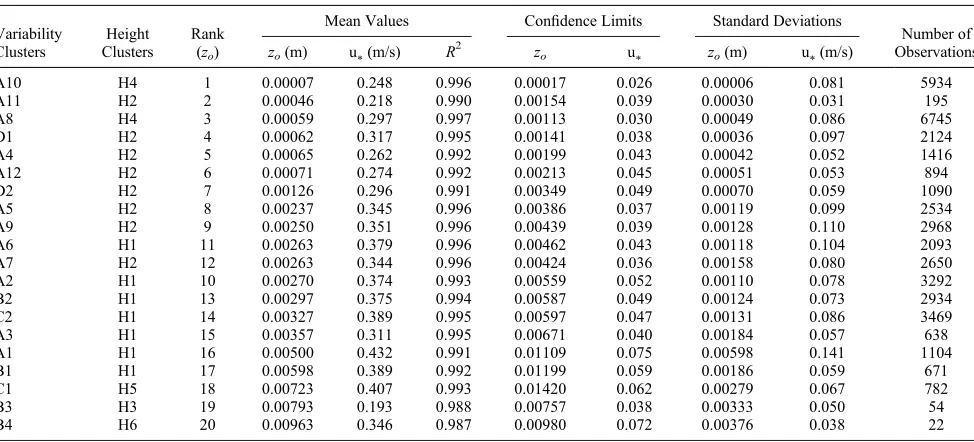
Table 3. Wind Data for Each Site Ordered byzoMagnitude

Variability Clusters

Height Clusters

Rank (zo)

Mean Values Confidence Limits Standard Deviations

Number of Observations zo(m) u_*(m/s) R

2

zo u_* zo(m) u_*(m/s)

A10 H4 1 0.00007 0.248 0.996 0.00017 0.026 0.00006 0.081 5934

A11 H2 2 0.00046 0.218 0.990 0.00154 0.039 0.00030 0.031 195

A8 H4 3 0.00059 0.297 0.997 0.00113 0.030 0.00049 0.086 6745

D1 H2 4 0.00062 0.317 0.995 0.00141 0.038 0.00036 0.097 2124

A4 H2 5 0.00065 0.262 0.992 0.00199 0.043 0.00042 0.052 1416

A12 H2 6 0.00071 0.274 0.992 0.00213 0.045 0.00051 0.053 894

D2 H2 7 0.00126 0.296 0.991 0.00349 0.049 0.00070 0.059 1090

A5 H2 8 0.00237 0.345 0.996 0.00386 0.037 0.00119 0.099 2534

A9 H2 9 0.00250 0.351 0.996 0.00439 0.039 0.00128 0.110 2968

A6 H1 11 0.00263 0.379 0.996 0.00462 0.043 0.00118 0.104 2093

A7 H2 12 0.00263 0.344 0.996 0.00424 0.036 0.00158 0.080 2650

A2 H1 10 0.00270 0.374 0.993 0.00559 0.052 0.00110 0.078 3292

B2 H1 13 0.00297 0.375 0.994 0.00587 0.049 0.00124 0.073 2934

C2 H1 14 0.00327 0.389 0.995 0.00597 0.047 0.00131 0.086 3469

A3 H1 15 0.00357 0.311 0.995 0.00671 0.040 0.00184 0.057 638

A1 H1 16 0.00500 0.432 0.991 0.01109 0.075 0.00598 0.141 1104

B1 H1 17 0.00598 0.389 0.992 0.01199 0.059 0.00186 0.059 671

C1 H5 18 0.00723 0.407 0.993 0.01420 0.062 0.00279 0.067 782

B3 H3 19 0.00793 0.193 0.988 0.00757 0.038 0.00333 0.050 54

where RSAis the areal roughness density based on surface

area, SAridgeis the actual surface area of each site, SAboxis

the planform area of the site, Vridgeis the element volume

above a plane intersecting the lowest surface point, and

Vboxis the volume of air within which the elements reside,

1 m above the lowest surface point.

[13] We assimilate all of the above methods to classify

TLS-measured surface element configurations both in mag-nitude, shape, and variability using cluster analysis and then determine multiple linear regression relationships between surface metrics andzoto identify which of these key surface

characteristics (magnitude, shape, or variability) has a greater influence on estimatingzo.

3. Study Sites and Field Methods

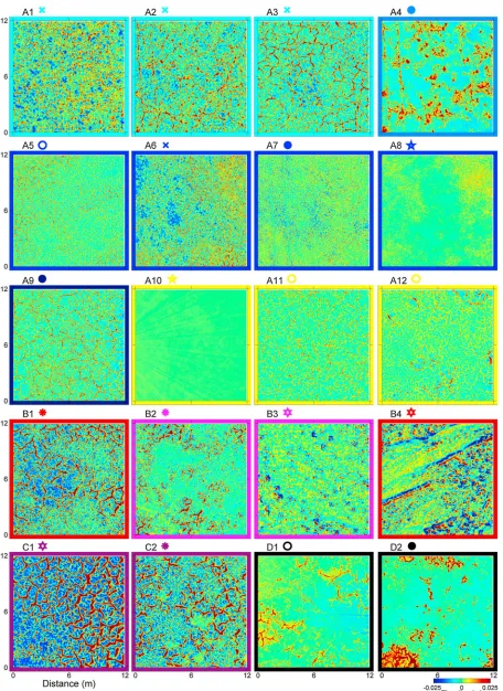
[14] Twenty surfaces spanning a range of element

magni-tudes (flat to cobbles) and pattern configurations (regular to ir-regular) typical of dust-emitting landscapes (Figure 1; Table 2) were measured using a Leica ScanStation TLS in July, August 2011, and August 2012. Eighteen surfaces were located on Sua Pan, part of the Makgadikgadi Salt Pan complex in central Botswana (20.5754°S, 25.959°E). Sua experiences ephemeral surfaceflooding [Eckardt et al., 2008] and is one of southern Africa’s most important aeolian dust source areas [Bryant et al., 2007;Prospero et al., 2002;Washington et al., 2003;

Zender and Kwon, 2005]. The pan surface comprises a polygon crust (Figures 1a and 1b) of varying morphology and in various states of formation and degradation. The measured surfaces ranged from newly formed, flat crust, to well-formed polygons (Figure 1b). A number of surfaces were degraded with broken and deflated ridges, and some surfaces contained a mix of flat, newly formed crust and extruding and broken crust ridges. Two further surfaces with larger

element heights were measured at Kotarjökull and Falljökull sandar in Southeast Iceland (63.925°N, 16.792°W and 63.950°N, 16.832°W, respectively) which are a major source of high-latitude dust [Prospero et al., 2012]. At Kotarjökull we sampled an inactive, stabilized terrace surface with rounded volcanic fluvial deposits. At Falljökull sandur we sampled the active surface, with braided river channels sur-rounding the measurement site and volcanicfluvial sediments (Figure 1c). Both sandar areflat and exposed to the dominant wind fetch from the south east for several kilometers.

[15] High-resolution surface topography was measured

with a specified resolution of 0.005 m at 30 m for the salt crust and 0.01 m at 50 m and 70 m for the Kotarjökull sandur and Falljökull sandur sites, respectively. Upwind of each in-strument setup for data analysis, 144 m2sections of data were extracted. Data were reduced to a digital elevation model (DEM) of 0.01 m grid resolution, by assigning the average elevation value in each cell to that grid. Mixed pixels were not noticeably influential in point cloud measurements due to the relatively flat surfaces and high incident angle. Replicate scans of the same surface area at two salt pan sites (flat and ridged) during the day indicated mean surface differ-ences less than 0.003 m, which is below the mean error values of 0.0032 to 0.0034 m recorded from modeled and measured Leica TLS data by Hodge [2010]. Empty cells were interpolated in Matlab (Mathworks Inc.) using the nat-ural neighbor (continuous convex hull triangulation) method. Occluded areas were limited to the ridge and rock sides fac-ing away from the TLS on the surfaces with taller elements. Analysis undertaken on independent 55 m squares pro-duced similar metric results, suggesting interpolation of away facing elements did not adversely influence analysis of the larger surface areas. Larger-scale surface gradients on the sandar were removed by subtracting the underlying

0 1 2 3 4 5 6 7 8 9 10

B1 B2 B3 B4 C1 C2 D1 D2 0

1 2 3 4 5 6 7 8 9 10

A1 A2 A3 A4 A5 A6 A7 A8 A9 A10 A11 A12

0 8000 16000 24000

spatial frequency (m−1₎

amplitude relative to A10

0 1000 2000 3000 4000 5000 6000

101 ₁₀0 ₁₀-1 ₁₀-2 ₁₀1 ₁₀0 ₁₀-1 ₁₀-2

101

100

10-1 ₁₀2 ₁₀-1 ₁₀0 ₁₀1 ₁₀2

wavelength (m)

b)Wavelet

a)Fourier transform

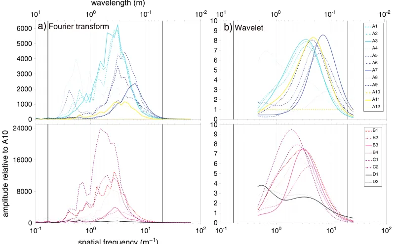
Figure 3. (a) Fourier transform and (b) wavelet spectra arranged and colored using variability cluster

surface calculated using a 0.26 m2moving window average. Manual measurements of surface bumps using the raw TLS point data along six transects for each sandur following the Gaussian bumpfitting methods ofKean and Smith [2006a, 2006b] produced similar mean height (difference<0.001 m) and wavelength (difference<0.05 m) values as the automated transects on the detrended surfaces.

[16] Wind speeds on Sua Pan were measured at four heights

above the surface (at 0.25 m, 0.47 m, 0.89 m, and 1.68 m) with Vector Instruments rotating cup anemometers (A-100R). Analysis was restricted to easterly wind measurements (45° to 135° from north; the dominant storm direction) within a 2-week period centered on the same day as the TLS measure-ments were collected at each site. At the sandur sites, wind speeds were measured at five heights above the surface (at 0.08 m, 0.48 m, 1.02 m, 1.69 m, and 2.4 m) with RM Young cup anemometers and wind measurements over 4 h periods were analyzed. All wind speed measurements from each site and location were averaged over 1 min to calculate shear velocity (u*) and aerodynamic roughness values (zo)

fol-lowing standard law of the wall profile methods [Oke, 1987]. Measurements werefiltered to minimize any buoyancy effects with a threshold for wind speed at the lowest anemometer height of 3 ms1_{and 1 ms}1_{for the salt pan and sandar,}

re-spectively. All instances where theR2values for the log-linear regression of height against wind speed to calculate u*andzo

that were below 0.98 were also discarded [Bauer et al., 1992;Namikas et al., 2003]. Table 3 indicates the number of measurements used for each calculation.

4. Spatial Variability in TLS-Measured Surface Roughness

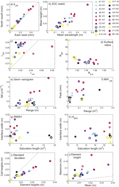
[17] The 20 measured surfaces covered a range of element

heights (0.001–0.036 m mean height and 0.007–0.199 m maximum heights using the zero-up-crossing method), ridge

spacing (0.058–0.536 m mean wavelength), and pattern variability (Figure 2).kLMvalues calculated in wind

perpen-dicular and parallel direction indicate that there was no dom-inant directional bias within the data (Figure 2a; correlation coefficient = 0.99,p<0.001). The mean wavelengths mea-sured by the zero-up-crossing transect method strongly corre-lated to the minimum wavelengths found using the Fourier transforms (Figures 2b and 3a; coefficient = 0.82). Wavelet peaks (Figure 3b) indicate the smallest wavelengths identi-fied by the Fourier analysis, and the wavelet peak widths span similar ranges, but the Fourier spectra are more advan-tageous as they identify individual wavelengths within the data set distribution and so are useful for identifying multiple scales of patterning across the surface.

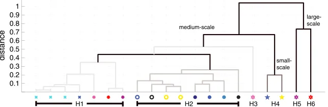
[18] The 20 surfaces were independently grouped using

clus-ter analysis into two sets to identify surfaces with similar pat-tern variability (Figure 4) or height characteristics (Figure 5) and to explore the relationships of these pattern types to aero-dynamic roughness. The metric sets used for each of the vari-ability and height clusters are defined a priori in Table 1, and planform plots of each surface arranged by pattern variability clusters are shown in Figure 6.

[19] The variability cluster analysis (Figures 4 and 6) identi-fied four main groups (based on greatest dendrogram distance gap). These groups (and subgroups) were qualitatively charac-terized by independent analysis of the normalized Fourier transform and wavelet spectra (Figure 3). Thefirst dendrogram arm separates regular (A, B and C) from irregular (D) surfaces. Group A is predominantly composed of uniform elements, Group B has occasional larger elements, and Group C consists of dominant larger-scale wavelengths. Within Group A, A1 to A3 have strong small-scale patterns, A5 to A9 have very weak large scale patterns, and A10 to A12 have occasional larger el-ements. A4 has a mix of patterns, indicated by multiple peaks of similar magnitude on the normalized Fourier transform spectra (Figure 3). Group B has larger elements and spacing

0.1 0.2 0.3 0.4 0.5 0.6 0.7 0.8 0.9 1

distance

large-scale

small-scale medium-scale

5 H 4 H 3 H 2

H 1

H H6

Figure 5. Dendrogram for height cluster groups (see Table 1 for list of contributing metrics). Colors

rep-resent variability clusters (Figure 4), and symbols correspond to height clustering. A1 A2 A3 A4 A5 A6 A7 A8 A9 A10 A11 A12 B1 B2 B3 B4 C1 C2 D1 D2 0.2

0.4 0.6 0.8 1 1.2 1.4 1.6

distance

Irregular Regular

dominant large-scale dominant

small-scale

occasional large elements uniform

elements

strong small-scale

pattern

weak large-scale pattern

large and small patches

occasional small elements mixed

pattern

generally than Group A, but it also has a mix of larger and smaller scale pattern types, organized in local patches, partic-ularly in the cases of B2 and B3 that have less intense medium scale Fourier transform peaks. Group C is dominated by large-scale elements and wavelengths and has the longest wave-length peaks within the Fourier and wavelet analyses. Group D consists of irregular elements (Figure 1a) with weak rela-tionships between both small and large wavelengths in both the Fourier and wavelet spectra. Visually, Group D consists of large elements in close proximity, isolated from other ele-ment assemblages byflat areas, as indicated by the larger sat-uration length for the RMSH moving window analysis compared to the other surfaces (Figure 2g).

[20] Clustering the surfaces using the height magnitude

met-rics from Table 1 produced six significant groups (Figure 5). The greatest dendrogram distances separated medium-scale groups (H1, H2, and H3) from small-scale (H4) and large-scale groups (H5 and H6).

[21] A number of metrics are particularly good at

distinguishing the different height and variability clusters. Maximum height within moving window separates the variability groups by saturation length and height groups by interface width (Figure 2h). Variability group D has a much larger RMSH saturation length than the rest of the surfaces,

but the height of its members (interface width) matches the re-lated height cluster groups (Figure 2g). Aside from the two sandur surfaces (B3/H3 and B4/H6),λ2-Doverpredicts

rough-ness density compared toλvol(Figure 2c). This is because the

sandur surfaces do not have the interconnected ridge pattern of the salt pan. For small heights (height cluster group H4), nonspatial and element height standard deviation are similar values, but as pattern magnitude increases (pattern variability group C), the standard deviation of element height increases at a greater rate than the nonspatial value (Figure 2i). Irrespective of pattern cluster group, the members of the larg-est height clusters (H5 and H6) are end-members for both mean and maximum element height (Figure 2j).

5. Aerodynamic Roughness Variability

[22] Mean and standard deviation values for wind profiles

measured at each site from the dominant wind direction are shown in Table 3. Aerodynamic roughness measurements in general followed the height cluster groups (Figure 5) and ranged from 7 105m at the smoothest site (A10/H4) to 9.6103_{m at the roughest site (B4/H6). H3 and H5 groups}

produced largerzovalues and group H2 generally produced

smallerzovalues. Shear velocity measurements ranged from Table 4. R2Values for Least Square Linear Regression Relationships Between the Natural Logs of Aerodynamic Roughness and the Surface Metrics; Asterisk IndicatespValue Below 0.002a

R2 Model Coefficients

Analysis

Dimension Metric

All Values

Excluding

Smooth Intercept Gradient

1-D Standard deviation of elevation distribution 0.75 0.58 0.65 1.37*

2-D Zero-up-crossing transects Height (mean) 0.79 0.65 0.28 1.33*

Height (max) 0.75 0.56 2.02 1.50* Height (std) 0.81 0.71 0.29 1.33* Ridge width 0.50 0.25 2.72 1.76* Ridge wavelength 0.60 0.38 3.43 1.89* Interridge spacing 0.67 0.50 1.82 1.89*

RBF 0.46 0.14 0.07 2.03*

λ2-D 0.51 0.19 0.73 2.10*

kLM 0.76 0.62 1.80 0.92*

Semivariogram Sill 0.79 0.67 0.60 0.67*

Range 0.07 0.08 6.26 0.73

3-D Moving window analysis Mean of elevation standard deviations Interface width 0.75 0.59 0.47 1.31* Saturation length 0.00 0.06 6.25 0.04 Standard deviation of elevation

standard deviations

Peak value 0.51 0.51 2.36 1.38*

Range 0.00 0.00 5.94 0.05

Root-mean-squared height (RMSH) Interface width 0.75 0.59 0.47 1.31* Saturation length 0.05 0.18 6.13 0.21 Maximum height Interface width 0.80 0.67 1.43 1.66* Saturation length 0.09 0.03 0.83 2.51 Fourier transform magnitude relative toflat surface 0.58 0.58 11.99 0.70*

dominant wavelength 0.15 0.15 6.26 0.35

Wavelet magnitude relative toflat surface 0.27 0.27 8.89 1.49

dominant wavelength 0.03 0.03 6.31 0.21

RSA 0.53 0.39 8.13 51.18*

λvol 0.79 0.66 0.01 1.55*

Height group 0.92 0.87 *

Shape group 0.86 0.78 *

Wavelength group 0.81 0.81 *

Variability group 0.86 0.86 *

0.19 to 0.43 ms1 _{and were not related to z}

o magnitude

(R2= 0.104). Confidence limits for shear velocities andzoranged

from 10 to 21% and 95 to 333% of the mean values, respectively.

6. Implications for Quantifying Aerodynamic Roughness of Complex Surfaces

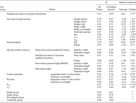
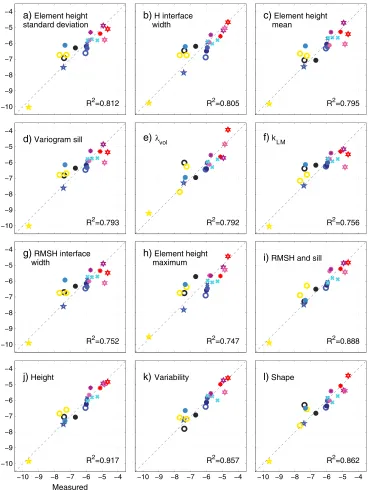
[23] The ability of different surface metrics to characterize

aerodynamic roughness is illustrated in Table 4 and Figure 7. In general, variations in aerodynamic roughness (zo) are

con-trolled more strongly by parameters that include some aspect

of surface roughness height in their metrics rather than surface roughness spacing. For example, metrics such as element mean height and standard deviation using the zero-up-crossing method, interface width of maximum height within a moving window, semivariogram sill, andλvolall haveR2values greater

than 0.79 when regressed againstzo(Figures 7a–7e). Surface

roughness descriptorskLM, RMSH interface width, and

maxi-mum element height also perform well (R2>0.74; Figures 7f– 7h). Of these metrics, the standard deviation of element heights, interface width of maximum height within a moving window, and semivariogram sill are less sensitive to the −10

−9 −8 −7 −6 −5 −4

a) Element height standard deviation

R2=0.812 R2=0.805

b)H interface width

c)Element height mean

R2=0.795

−10 −9 −8 −7 −6 −5 −4

d)Variogram sill

R2=0.793

e) λ_vol

R2=0.792

f)k

LM

R2=0.756

−10 −9 −8 −7 −6 −5 −4

R2=0.752

g)RMSH interface width

h)Element height maximum

R2=0.747 R2=0.888

i)RMSH and sill

−10 −9 −8 −7 −6 −5 −4 −10

−9 −8 −7 −6 −5 −4

j)Height

Predicted

Measured

R2=0.917

−10 −9 −8 −7 −6 −5 −4 k) Variability

R2=0.857

−10 −9 −8 −7 −6 −5 −4 l)Shape

R2=0.862

Figure 7. (a–i) Measured and predicted values of the natural log of aerodynamic roughness for the best

exclusion of the smooth surface (R2_{>0.66; Table 4). Multiple}

linear regressions were performed on each of the groups from Table 1 to determine the relationships between shape, height, variability, and wavelength groups (Figures 7j–7l).

lnð Þ ¼zo 0:45 heightþ0:37 variabilityþ0:20 shape

þ0:10 wavelength

þ0:72 R2¼0:90;p<1106 (9)

lnð Þ ¼zo 0:58 heightþ0:50 variability

þ0:48 R2¼0:90;p<1107 (10)

[24] Coefficients andR2values from the multiple linear

re-gressions confirm that height is the most significant of the pattern descriptors with respect to aerodynamic roughness, both for the combination of all metric descriptors (equation (9)) and the combination of height and variability groups only (equation (10)). When a surface consists of larger rough-ness elements (B3/H3, C1/H5, and B4/H6), the best metric predictors are the interface width of maximum height and element maximum height (Figures 7b and 7h). This agrees with wind tunnel studies that have found maximum height out-performs mean height for nonuniform blocks [Cheng and Castro, 2002;Hagishima et al., 2009]. However, these maxi-mum height-based metrics underpredict or overpredictzoon

surfaces with moderate element heights but underlying, weak large-scale pattern variability or irregularity (A4/H2, A11/ H2, A12/H2, D1/H2, and D2/H2). Modelingλvol(Figure 7e)

reduces the residual error for some of these surfaces, but has outliers relating to the height groups (D1/H2 and A12/H2), and is less able to predictzoon some larger surfaces (H5 and

H6). The other highly correlated metrics all perform similarly in terms of ability to predict zo on a uniform surface with

small-scale patterns (A1 to A3, A6 to A9, and B1 to B2). Moreover, our results suggest that if surfaces measured at high resolution are quantified using the suite of metrics discussed in this paper, over 90% of the variance can be explained for aero-dynamic roughness estimation.

[25] The combination of RMSH and variogram sill (Figure 7i)

performs best at reducing pattern specific outliers, but these metrics require detailed surface measurements. More common metrics typically measured using field transects include

element height (mean, maximum, and standard deviation) and element width or wavelength (spacing). If we consider only pairs of these commonly measured metrics, where each pair consists of one vertical and one horizontal metric, then irrespective of the exact pairing, multiple linear regressions generate larger coefficients for the height (vertical) component.

lnð Þ ¼zo 1:66 lnðHmeanÞ 0:63 lnðWmeanÞ

0:08 R2¼0:81;p<1106 (12)

lnð Þ ¼zo 1:48 lnðHmaxÞ 0:04 lnðWmeanÞ

2:0 R2¼0:75;p<1105 (13)

[26] where Hmean is the mean element height across all

transects;Hmaxis the maximum element height for each

tran-sect, averaged across all transects, and Wmean is the mean

element width.

[27] The inclusion of ridge width or wavelength does not

improve the R2_{value from regressions that include only a}

single height metric by more than 4%. This suggests that in environments where data are limited, an accurate measure-ment of the mean or maximum elemeasure-ment height may be suffi -cient to explain most of the variance in the aerodynamic roughness height.

[28] Roughness density (λ) is the most common shape

de-scriptor used to relate surface and aerodynamic roughness. Figure 8 compares values of mean height,λ, and standard de-viation of height from previous studies of unvegetated sur-faces (filtered for appropriate methodologies), and our study, resulting inR2values of 0.54, 0.33, and 0.47, respec-tively (n= 58, 41, 29). Some of the variation can be explained by the differences in methodology.Greeley et al. [1995] used a laser profiler, but the profile length was 1.2 m along each side of a triangle, so this method is likely to underpredict the presence of large roughness elements, as is evident by the larger residuals for higherzovalues.Gillies[1994] used

a laser scanner to characterize the surface, but this study was undertaken in a wind tunnel, which may explain the overprediction for very small values ofzo.MacKinnon et al.

[2004] assumed a cylindrical shape for roughness elements thatzowas measured over and, when this data set is excluded, R2values improve to 0.59, 0.69, and 0.74 for mean height,λ, −8 −7 −6 −5 −4 −3 −2 −1

−10 −9 −8 −7 −6 −5 −4 −3

ln(mean height)

ln(z

o

)

Lancaster (2004) TLS data (this study) Greeley et al. (1995) MacKinnon et al. (2004) Xian et al. (2002) Gillies ssp (1994) Gillies pro (1994)

−8 −7 −6 −5 −4 −3 −2 −1

ln(λ)

−8 −7 −6 −5 −4 −3 −2

ln(height standard deviation)

) c )

b )

a

Figure 8. Comparison of (a) mean height, (b) lambda, and (c) standard deviation of element height values

from TLS and published data [Gillies, 1994;Greeley et al., 1995;Lancaster, 2004;MacKinnon et al., 2004;

and standard deviation of height, respectively (n= 53, 36, 24).

Lancaster [2004] only examined elements with a diameter greater than 10 cm, resulting in underprediction of mean ele-ment height and λ for small surface roughness and is best modeled using maximum (equation (13)) rather than mean el-ement height (equation (12)). If these points are also excluded, then theR2value for mean height increases to 0.65 (n= 37). This suggests that if element heights are measured to high pre-cision, mean height performs as well or better thanλ2-Dfor

predictingzo. This agrees with studies of much larger

rough-ness elements that point to the need to include more weighting of element height rather than only roughness density when predicting sediment transport over complex surfaces [Gillies and Lancaster, 2013]. While our study has highlighted the im-portance of height characterization forzoestimation, further

re-search is needed into sedimentation patterns over these surfaces, and TLS is a useful technique to map these patterns at high resolution.

7. Conclusions

[29] Ourfindings show that when a surface is measured at

high (mm scale) spatial resolution, any metric combination that includes a height-related component will be able to pre-dict aerodynamic roughness (zo), but the optimal choice

de-pends on the pattern variability of the surface. For surfaces with large elements, or that exhibit mixed homogenous patches of large and small roughness elements, maximum height is the best predictor ofzowhile for more uniform

sur-faces, mean element height orλvolshould be used to predict zo. Multiple linear regressions indicate that, in general, height

is the most significant descriptor, and wavelength is less im-portant for continuous roughness elements found on crusted or rocky surfaces. Where it is possible to measure a complete DEM of surface elevations, a combination of variogram sill and RMSH is the best combination for aerodynamic rough-ness estimates as this combination is less sensitive to pattern variability. However, our data also suggest that the height of surface roughness provides a good explanation (R2>0.79) for most of the variance in aerodynamic roughness (zo) and

performs at least as well as the more complex roughness den-sity metrics. Aerodynamic roughness (zo) is a fundamental

parameter in wind erosion and dust emission modeling, crit-ical in the calculation of shear velocity (u*) and erosion

thresholds. This study is thefirst to recognize the significance of height for estimating aerodynamic roughness when small-scale complex surface roughness is accurately quantified, irrespective of comparator metric choice. This has very sig-nificant implications for the development of aerodynamic roughness predictors which are fundamental to the efficiency of wind erosion models, and, particularly, dust emission schemes in climate models.

[30] Acknowledgments. The Botswanafieldwork was partly funded by NERC as part of the DO4models project (NE/H021841/1), with travel support for Nield from a World University Network mobility grant and a University of Southampton SIRDF grant. The Iceland component was funded by a Royal Society Research Grant awarded to Nield (RG090467). Vircavs was supported by the EPSRC Vacation Bursary Scheme (EP/ J500537/1 Doctoral Training Account (University of Southampton)). Data processing was undertaken using the IRIDIS High Performance Computing Facility at the University of Southampton. R.T. Wilson is thanked for his assistance with the surface area calculations, J.A. Gillies, A.C.W. Baas, and C.S.B. Grimmond for insightful discussions, and two anonymous reviewers for helpful suggestions.

References

Anderson, K., J. Bennie, and A. Wetherelt (2010), Laser scanning offine scale pattern along a hydrological gradient in a peatland ecosystem, Landscape Ecol.,25(3), 477–492.

Antonarakis, A. S., K. S. Richards, J. Brasington, and M. Bithell (2009), Leafless roughness of complex tree morphology using terrestrial lidar, Water Resour. Res.,45, W10401, doi:10.1029/2008WR007666. Bauer, B. O., D. J. Sherman, and J. F. Wolcott (1992), Sources of uncertainty

in shear-stress and roughness length estimates derived from velocity profiles,Professional Geogr.,44(4), 453–464.

Blumberg, D. G., and R. Greeley (1993), Field studies of aerodynamic roughness length,J. Arid Environ.,25, 39–48.

Booth, A. M., J. J. Roering, and J. T. Perron (2009), Automated landslide mapping using spectral analysis and high-resolution topographic data: Puget Sound lowlands, Washington, and Portland Hills, Oregon, Geomorphology,109(3-4), 132–147.

Brock, B. W., I. C. Willis, and M. J. Shaw (2006), Measurement and param-eterization of aerodynamic roughness length variations at Haut Glacier d’Arolla, Switzerland,J. Glaciol.,52(177), 281–297.

Brown, O. W., and C. H. Hugenholtz (2011), Estimating aerodynamic roughness (zo) in mixed grassland prairie with airborne LiDAR,Can. J. Remote Sens.,37(4), 422–428.

Brown, S., W. G. Nickling, and J. A. Gillies (2008), A wind tunnel examina-tion of shear stress partiexamina-tioning for an assortment of surface roughness dis-tributions,J. Geophys. Res.,113, F02S06, doi:10.1029/2007JF000790. Bryant, R. G., G. R. Bigg, N. M. Mahowald, F. D. Eckardt, and S. G. Ross

(2007), Dust emission response to climate in southern Africa,J. Geophys. Res.,112, D09207, doi:10.1029/2005JD007025.

Buckley, S. J., J. A. Howell, H. D. Enge, and T. H. Kurz (2008), Terrestrial laser scanning in geology: Data acquisition, processing and accuracy considerations,J. Geol. Soc.,165, 625–638.

Bullard, J. E., S. P. Harrison, M. C. Baddock, N. Drake, T. E. Gill, G. McTainsh, and Y. Sun (2011), Preferential dust sources: A geomorpho-logical classification designed for use in global dust-cycle models, J. Geophys. Res.,116, F04034, doi:10.1029/2011JF002061.

Castro, I. P., H. Cheng, and R. Reynolds (2006), Turbulence over urban-type roughness: Deductions from wind-tunnel measurements,Boundary Layer Meteorol.,118(1), 109–131.

Cheng, H., and I. P. Castro (2002), Near wallflow over urban-like rough-ness,Boundary Layer Meteorol.,104(2), 229–259.

Cheng, H., P. Hayden, A. G. Robins, and I. P. Castro (2007), Flow over cube arrays of different packing densities,J. Wind Eng. Ind. Aerodynamics, 95(8), 715–740.

Croft, H., K. Anderson, and N. J. Kuhn (2012), Reflectance anisotropy for measuring soil surface roughness of multiple soil types,CATENA,93, 87–96.

Croft, H., K. Anderson, R. E. Brazier, and N. J. Kuhn (2013), Modellingfine scale soil surface structure using geostatistics,Water Resour. Res.,49, 1858–1870, doi:10.1002/wrcr.20172.

Darmenova, K., I. N. Sokolik, Y. Shao, B. Marticorena, and G. Bergametti (2009), Development of a physically based dust emission module within the Weather Research and Forecasting (WRF) model: Assessment of dust emission parameterizations and input parameters for source regions in Central and East Asia,J. Geophys. Res., 114, D14201, doi:10.1029/ 2008JD011236.

Eamer, J. B. R., and I. J. Walker (2010), Quantifying sand storage capacity of large woody debris on beaches using LiDAR,Geomorphology,118, 33–47. Eckardt, F. D., R. G. Bryant, G. McCulloch, B. Spiro, and W. W. Wood (2008), The hydrochemistry of a semi-arid pan basin case study: Sua Pan, Makgadikgadi, Botswana,Appl. Geochem.,23(6), 1563–1580. Eitel, J. U. H., C. J. Williams, L. A. Vierling, O. Z. Al-Hamdan, and

F. B. Pierson (2011), Suitability of terrestrial laser scanning for studying surface roughness effects on concentrated flow erosion processes in rangelands,CATENA,87(3), 398–407.

Fardin, N., Q. Feng, and O. Stephansson (2004), Application of a new in situ 3D laser scanner to study the scale effect on the rock joint surface rough-ness,Int. J. Rock Mech. Mining Sci.,41(2), 329–335.

Frankel, K. L., and J. F. Dolan (2007), Characterizing arid region alluvial fan surface roughness with airborne laser swath mapping digital topographic data,J. Geophys. Res.,112, F02025, doi:10.1029/2006JF000644. Gillies, J. A. (1994), A wind tunnel study of the relationships between

com-plex surface roughness form,flow geometry and shearing stress, PhD thesis, Department of Geography, University of Guelph.

Gillies, J. A., W. G. Nickling, and J. King (2007), Shear stress partitioning in large patches of roughness in the atmospheric inertial sublayer,Boundary Layer Meteorol.,122(2), 367–396.

Glenn, N. F., D. R. Streutker, D. J. Chadwick, G. D. Thackray, and S. J. Dorsch (2006), Analysis of LiDAR-derived topographic information for characterizing and differentiating landslide morphology and activity, Geomorphology,73(1-2), 131–148.

Goda, Y. (2000),Random Seas and Design of Maritime Structures, World Scientific, Singapore.

Grant, P. F., and W. G. Nickling (1998), Directfield measurement of wind drag on vegetation for application to windbreak design and modelling, Land Degradation Dev.,9(1), 57–66.

Greeley, R., D. G. Blumberg, A. R. Dobrovolskis, L. R. Gaddis, J. D. Iversen, N. Lancaster, K. R. Rasmussen, R. S. Saunders, S. D. Wall, and B. R. White (1995), Potential transport of windblown sand: Influence of surface rough-ness and assessment with radar data, inDesert Aeolian Processes, edited by V. P. Tchakerian, pp. 75–99, Chapman and Hall, New York.

Greeley, R., D. G. Blumberg, J. F. Mchone, A. Dobrovolskis, J. D. Iversen, N. Lancaster, K. R. Rasmussen, S. D. Wall, and B. R. White (1997), Applications of spaceborne radar laboratory data to the study of aeolian processes,J. Geophys. Res.,102(E5), 10,971–10,983.

Grimmond, C. S. B., and T. R. Oke (1999), Aerodynamic properties of urban areas derived, from analysis of surface form,J. Appl. Meteorol.,38(9), 1262–1292.

Hagishima, A., J. Tanimoto, K. Nagayama, and S. Meno (2009), Aerodynamic parameters of regular arrays of rectangular blocks with various geometries, Boundary Layer Meteorol.,132(2), 315–337.

Harrison, J. M., and C. P. Lo (1996), PC-based two-dimensional discrete Fourier transform programs for terrain analysis,Comp. Geosci.,22(4), 419–424.

Haubrock, S. N., M. Kuhnert, S. Chabrillat, A. Guntner, and H. Kaufmann (2009), Spatiotemporal variations of soil surface roughness from in-situ la-ser scanning,CATENA,79(2), 128–139.

Hodge, R. A. (2010), Using simulated Terrestrial Laser Scanning to analyse errors in high-resolution scan data of irregular surfaces, ISPRS J. Photogramm. Remote Sens.,65(2), 227–240.

Hodge, R., J. Brasington, and K. S. Richards (2009), Analysing laser-scanned digital terrain models of gravel bed surfaces: Linking morphology to sediment transport processes and hydraulics,Sedimentology,56(7), 2024–2043.

Huang, G. H., and C. K. Wang (2012), Multiscale geostatistical estimation of gravel-bed roughness from Terrestrial and Airborne Laser Scanning, Geosci. Remote Sens. Lett. IEEE,9(6), 1084–1088.

Hugenholtz, C. H., O. W. Brown, and T. E. Barchyn (2013), Estimating aerodynamic roughness (z0) from terrestrial laser scanning point cloud data over un-vegetated surfaces,Aeolian Res.,10, 161–169.

Jenness, J. S. (2004), Calculating landscape surface area from digital eleva-tion models,Wildlife Soc. Bull.,32(3), 829–839.

Kaasalainen, S., H. Kaartinen, A. Kukko, K. Anttila, and A. Krooks (2011), Application of mobile laser scanning in snow cover profiling,Cryosphere, 5(1), 135–138.

Kean, J. W., and J. D. Smith (2006a), Form drag in rivers due to small-scale natural topographic features: 1. Regular sequences,J. Geophys. Res.,111, F04009, doi:10.1029/2006JF000467.

Kean, J. W., and J. D. Smith (2006b), Form drag in rivers due to small-scale natural topographic features: 2. Irregular sequences,J. Geophys. Res.,111, F04010, doi:10.1029/2006JF000490.

Khoshelham, K., D. Altundag, D. Ngan-Tillard, and M. Menenti (2011), Influence of range measurement noise on roughness characterization of rock surfaces using terrestrial laser scanning,Int. J. Rock Mech. Mining Sci.,48(8), 1215–1223.

King, J., W. G. Nickling, and J. A. Gillies (2006), Aeolian shear stress ratio measurements within mesquite-dominated landscapes of the Chihuahuan Desert, New Mexico, USA,Geomorphology,82(3-4), 229–244. King, J., W. G. Nickling, and J. A. Gillies (2008), Investigations of the

law-of-the-wall over sparse roughness elements, J. Geophys. Res., 113, F02S07, doi:10.1029/2007JF000804.

Lancaster, N. (2004), Relations between aerodynamic and surface roughness in a hyper-arid cold desert: Mcmurdo Dry Valleys, Antarctica,Earth Surf. Processes Landforms,29(7), 853–867.

Lancaster, N., and A. Baas (1998), Influence of vegetation cover on sand transport by wind: Field studies at Owens Lake, California,Earth Surf. Processes Landforms,23(1), 69–82.

Lancaster, N., W. G. Nickling, and J. A. Gillies (2010), Sand transport by wind on complex surfaces: Field studies in the McMurdo Dry Valleys, Antarctica,J. Geophys. Res.,115, F03027, doi:10.1029/2009JF001408. Laurent, B., B. Marticorena, G. Bergametti, P. Chazette, F. Maignan, and

C. Schmechtig (2005), Simulation of the mineral dust emission frequen-cies from desert areas of China and Mongolia using an aerodynamic roughness length map derived from the POLDER/ADEOS 1 surface prod-ucts,J. Geophys. Res.,110, D18S04, doi:10.1029/2004JD005013. Lettau, H. (1969), Note on aerodynamic roughness-parameter estimation on

the basis of roughness-element description, pp. 828–832.

Lyles, L., and B. E. Allison (1979), Wind profile parameters and turbulence intensity over several roughness element geometries,Trans.Asae,22(2), 334–343.

Lyons, A. P., W. L. J. Fox, T. Hasiotis, and E. Pouliquen (2002), Characterization of the two-dimensional roughness of wave-rippled seafloors using digital photogrammetry,Oceanic Eng. IEEE J.,27(3), 515–524.

MacKinnon, D. J., G. D. Clow, R. K. Tigges, R. L. Reynolds, and P. S. Chavez (2004), Comparison of aerodynamically and model-derived roughness lengths (z(o)) over diverse surfaces, central Mojave Desert, California, USA,Geomorphology,63(1-2), 103–113.

Mahowald, N. M., R. G. Bryant, J. del Corral, and L. Steinberger (2003), Ephemeral lakes and desert dust sources,Geophys. Res. Lett., 30(2), 1074, doi:10.1029/2002GL016041.

Manes, C., M. Guala, H. Löwe, S. Bartlett, L. Egli, and M. Lehning (2008), Statistical properties of fresh snow roughness,Water Resour. Res.,44, W11407, doi:10.1029/2007WR006689.

Marticorena, B., and G. Bergametti (1995), Modeling the atmospheric dust cycle: 1. Design of a soil-derived dust emission scheme,J. Geophys. Res., 100(D8), 16,415–16,430.

Marticorena, B., et al. (2006), Surface and aerodynamic roughness in arid and semiarid areas and their relation to radar backscatter coefficient, J. Geophys. Res.,111, F03017, doi:10.1029/2006JF000462.

Millward-Hopkins, J. T., A. S. Tomlin, L. Ma, D. Ingham, and M. Pourkashanian (2011), Estimating aerodynamic parameters of urban-like surfaces with heterogeneous building heights,Boundary Layer Meteorol., 141(3), 443–465.

Munro, D. S. (1989), Surfaceroughness and bulk heattransfer on a glacier -Comparison with eddy-correlation,J. Glaciol.,35(121), 343–348. Nakayama, H., T. Takemi, and H. Nagai (2011), LES analysis of the

aerody-namic surface properties for turbulentflows over building arrays with various geometries,J. Appl. Meteorol. Climatol.,50(8), 1692–1712. Namikas, S. L., B. O. Bauer, and D. J. Sherman (2003), Influence of

averag-ing interval on shear velocity estimates for aeolian transport modelaverag-ing, Geomorphology,53(3-4), 235–246.

Nield, J. M., and G. F. S. Wiggs (2011), The application of terrestrial laser scanning to aeolian saltation cloud measurement and its response to chang-ing surface moisture,Earth Surf. Processes Landforms,36(2), 273–278. Nield, J. M., G. F. S. Wiggs, and R. S. Squirrell (2011), Aeolian sand strip

mobility and protodune development on a drying beach: Examining sur-face moisture and sursur-face roughness patterns measured by terrestrial laser scanning,Earth Surf. Processes Landforms,36(4), 513–522.

Nield, J. M., R. C. Chiverrell, S. E. Darby, J. Leyland, L. H. Vircavs, and B. Jacobs (2013), Complex spatial feedbacks of tephra redistribution, ice melt and surface roughness modulate ablation on tephra covered glaciers, Earth Surf. Processes Landforms,38, 94–102.

Oke, T. R. (1987),Boundary Layer Climates, Routledge, London. Paul-Limoges, E., A. Christen, N. C. Coops, T. A. Black, and

J. A. Trofymow (2013), Estimation of aerodynamic roughness of a harvested Douglas-fir forest using airborne LiDAR, Remote Sens. Environ.,136, 225–233.

Perron, J. T., J. W. Kirchner, and W. E. Dietrich (2008), Spectral signatures of characteristic spatial scales and nonfractal structure in landscapes, J. Geophys. Res.,113, F04003, doi:10.1029/2007JF000866.

Prigent, C., I. Tegen, F. Aires, B. Marticorena, and M. Zribi (2005), Estimation of the aerodynamic roughness length in arid and semi-arid regions over the globe with the ERS scatterometer,J. Geophys. Res., 110, D09205, doi:10.1029/2004JD005370.

Prospero, J. M., P. Ginoux, O. Torres, S. E. Nicholson, and T. E. Gill (2002), Environmental characterization of global sources of atmospheric soil dust identified with the Nimbus 7 Total Ozone Mapping Spectrometer (TOMS) absorbing aerosol product, Rev. Geophys., 40(1), 1002, doi:10.1029/ 2000RG000095.

Prospero, J. M., J. E. Bullard, and R. Hodgkins (2012), High-latitude dust over the North Atlantic: Inputs from Icelandic proglacial dust storms, Science,335(6072), 1078–1082.

Raupach, M. R. (1992), Drag and drag partition on rough surfaces,Boundary Layer Meteorol.,60(4), 375–395.

Raupach, M. R., R. A. Antonia, and S. Rajagopalan (1991), Rough-wall turbulent boundary layers,Appl. Mech. Rev.,44(1), 1–25.

Raupach, M. R., D. A. Gillette, and J. F. Leys (1993), The effect of rough-ness elements on wind erosion threshold, J. Geophys. Res., 98(D2), 3023–3029.

Rodriguez-Caballero, E., Y. Canton, S. Chamizo, A. Afana, and A. Sole-Benet (2012), Effects of biological soil crusts on surface roughness and implica-tions for runoff and erosion,Geomorphology,145, 81–89.

Rotach, M. W. (1995), Profiles of turbulence statistics in and above an urban street canyon,Atmos. Environ.,29(13), 1473–1486.

with LiDAR-derived landscape surface roughness following wildfire, Geomorphology,119(1-2), 135–145.

Sankey, J. B., J. U. H. Eitel, N. F. Glenn, M. J. Germino, and L. A. Vierling (2011), Quantifying relationships of burning, roughness, and potential dust emission with laser altimetry of soil surfaces at submeter scales, Geomorphology,135(1-2), 181–190.

Sankey, J. B., S. Ravi, C. S. A. Wallace, R. H. Webb, and T. E. Huxman (2012), Quantifying soil surface change in degraded drylands: Shrub encroachment and effects offire and vegetation removal in a desert grassland, J. Geophys. Res., 117, G02025, doi:10.1029/ 2012JG002002.

Schirmer, M., and M. Lehning (2011), Persistence in intra-annual snow depth distribution: 2. Fractal analysis of snow depth development,Water Resour. Res.,47, W09517, doi:10.1029/2010WR009429.

Shaw, P. A., and R. G. Bryant (2011), Pans, playas and salt lakes, inArid Zone Geomorphology, pp. 373–401, John Wiley, Ltd., Chichester, West Sussex, U. K.

Smith, M. W., N. J. Cox, and L. J. Bracken (2011), Terrestrial laser scanning soil surfaces: Afield methodology to examine soil surface roughness and overlandflow hydraulics,Hydrol. Processes,25(6), 842–860.

Washington, R., M. Todd, N. J. Middleton, and A. S. Goudie (2003), Dust-storm source areas determined by the total ozone monitoring

spectrometer and surface observations,Ann. Assoc. Am. Geogr.,93(2), 297–313.

Weligepolage, K., A. S. M. Gieske, and Z. Su (2012), Surface roughness analysis of a conifer forest canopy with airborne and terrestrial laser scanning tech-niques,Int. J. Appl. Earth Observation Geoinformation,14(1), 192–203. Wiggs, G., and P. Holmes (2011), Dynamic controls on wind erosion and

dust generation on west-central Free State agricultural land, South Africa,Earth Surf. Processes Landforms,36(6), 827–838.

Wirz, V., M. Schirmer, S. Gruber, and M. Lehning (2011), Spatio-temporal measurements and analysis of snow depth in a rock face,Cryosphere,5(4), 893–905.

Wolfe, S. A., and W. G. Nickling (1993), The protective role of sparse vegetation in wind erosion,Prog. Phys. Geogr.,17(1), 50–68.

Xue, X., T. Wang, Q. W. Sun, and W. M. Zhang (2002), Field and wind-tunnel studies of aerodynamic roughness length, Boundary Layer Meteorol., 104(1), 151–163.

Zaki, S. A., A. Hagishima, J. Tanimoto, and N. Ikegaya (2011), Aerodynamic parameters of urban building arrays with random geome-tries,Boundary Layer Meteorol.,138(1), 99–120.