White Rose Research Online URL for this paper:
http://eprints.whiterose.ac.uk/43561/
Article:
Feldpausch, TR, Banin, L, Phillips, OL et al. (7 more authors) (2011) Height-diameter
allometry of tropical forest trees. Biogeosciences, 8 (5). 1081 - 1106 . ISSN 1726-4170
https://doi.org/10.5194/bg-8-1081-2011
[email protected] https://eprints.whiterose.ac.uk/ Reuse
See Attached Takedown
If you consider content in White Rose Research Online to be in breach of UK law, please notify us by
www.biogeosciences.net/8/1081/2011/ doi:10.5194/bg-8-1081-2011
© Author(s) 2011. CC Attribution 3.0 License.
Biogeosciences
Height-diameter allometry of tropical forest trees
T. R. Feldpausch1,*, L. Banin1,*, O. L. Phillips1, T. R. Baker1, S. L. Lewis1, C. A. Quesada1,2, K. Affum-Baffoe3, E. J. M. M. Arets4,5, N. J. Berry1,**, M. Bird6,***, E. S. Brondizio7, P. de Camargo8, J. Chave9, G. Djagbletey10, T. F. Domingues11,****, M. Drescher5,12, P. M. Fearnside2, M. B. Franc¸a2, N. M. Fyllas1, G. Lopez-Gonzalez1, A. Hladik13, N. Higuchi2, M. O. Hunter14, Y. Iida15, K. A. Salim16, A. R. Kassim17, M. Keller14,18, J. Kemp19,
D. A. King20, J. C. Lovett21, B. S. Marimon22, B. H. Marimon-Junior22, E. Lenza22, A. R. Marshall23, D. J. Metcalfe24, E. T. A. Mitchard11, E. F. Moran7, B. W. Nelson2, R. Nilus25, E. M. Nogueira2, M. Palace14, S. Pati ˜no1, 26,
K. S.-H. Peh1,*****, M. T. Raventos***, J. M. Reitsma27, G. Saiz6,***, F. Schrodt1, B. Sonk´e28, H. E. Taedoumg28, S. Tan29, L. White30,******, H. W¨oll31, and J. Lloyd1,***
1Earth and Biosphere Institute, School of Geography, University of Leeds, Leeds, LS2 9JT, UK
2Instituto Nacional de Pesquisas da Amazonia (INPA), Manaus, Brazil
3Forestry Commission of Ghana, P.O. Box 1457, Kumasi, Ghana
4Centre for Ecosystem Studies, Alterra, Wageningen Univ. and Research Centre, 6700 AA, Wageningen, The Netherlands
5Programa de Manejo de Bosques de la Amazonia Boliviana (PROMAB), P.O. Box 107, Riberalta, Bolivia
6School of Geography and Geosciences, Univ. of St. Andrews, KY16 9AL, UK
7Department of Anthropology and the Anthropological Center for Training and Research on Global Environmental Change,
Indiana University, Bloomington, USA
8Centro de Energia Nuclear na Agricultura, Av. Centen˜ario, 303 CEP: 13400-970, Piracicaba, S˜ao Paulo, Brazil
9Universite Paul Sabatier/CNRS, Laboratoire EDB UMR 5174, batiment 4R3, 31062 Toulouse, France
10Forest Research Institute of Ghana (FORIG), Kumasi, Ghana
11School of GeoSciences, University of Edinburgh, Drummond St, Edinburgh, EH8 9XP, UK
12School of Planning, University of Waterloo, 200 University Avenue West, Waterloo, ON N2L 3G1, Canada
13Eco-anthropologie et Ethnobiologie, D’epartement Hommes, Natures, Soci’et’es, MNHN, 4, avenue du Petit Chˆateau
91800 Brunoy, France
14Complex Systems Research Center, Univ. of New Hampshire, Durham, NH, 03824, USA
15Graduate School of Environmental Science, Hokkaido University, Sapporo, 060-0810, Japan
16Kuala Belalong Field Studies Centre, Universiti Brunei Darussalam, Biology Department, Jalan Tungku Link, BE1410,
Brunei Darussalam
17Forest Research Institute Malaysia (FRIM), 52109 Kepong, Selangor Darul Ehsan, Malaysia
18Int. Institute of Tropical Forestry, USDA Forest Service, San Juan, 00926, Puerto Rico
19Queensland Herbarium, Department of Environment and Resource Management, Townsville QLD 4810, Australia
20Biological and Ecological Engineering, Oregon State University, Corvallis, OR 97331, USA
21CSTM – Twente Centre for Studies in Technology and Sustainable Development, University of Twente; Postbus 217;
7500 AE; Enschede, The Netherlands
22Universidade do Estado de Mato Grosso, Caixa Postal 08, CEP 78690-000, Nova Xavantina, MT, Brazil
23CIRCLE, Environment Department, University of York, UK, and Flamingo Land, North Yorkshire, UK
24CSIRO Ecosystem Sciences, Tropical Forest Research Centre, Atherton, QLD 4883, Australia
25Forest Research Centre, Sabah Forestry Department, Sandakan, 90715, Malaysia
26Universidad Nacional de Colombia sede Amazonia, Km 2 v´ıa Tarapac´a, Leticia, Amazonas, Colombia
27Bureau Waardenburg bv, P.O. Box 365, 4100 AJ Culemborg, The Netherlands
28Plant Systematic and Ecology Laboratory, Department of Biology, Higher Teachers Training College, University of
Yaounde I, P.O. Box 047 Yaounde Cameroon
Correspondence to:
29Sarawak Forestry Corporation, Kuching, Sarawak, Malaysia
30Institut de Recherche en Ecologie Tropicale (IRET), BP 7847, Libreville, Gabon
31Sommersbergseestr. 291, 8990 Bad Aussee, Austria
∗These authors contributed equally to this work.
∗∗now at: Ecometrica, Unit 3B Kittle Yards, Edinburgh, EH9 1PJ, UK
∗∗∗now at: School of Earth and Environmental Science, James Cook University, P.O. Box 6811, Cairns,QLD 4870, Australia ∗∗∗∗now at: Instituto de Astronomia, Geof´ısica e Ciˆencias Atmosf´ericas – Universidade de S˜ao Paulo, 05508-090, Brasil ∗∗∗∗∗now at: Dept. of Zoology, Univ. of Cambridge, Downing Street, Cambridge, CB2 3EJ, UK
∗∗∗∗∗∗now at: Agence Nationale des Parcs Nationaux, Pr´esidence de la R´epublique, R´epublique Gabonaise, Gabon
Received: 13 September 2010 – Published in Biogeosciences Discuss.: 25 October 2010 Revised: 11 March 2011 – Accepted: 21 March 2011 – Published: 5 May 2011
Abstract. Tropical tree height-diameter (H:D) relationships may vary by forest type and region making large-scale es-timates of above-ground biomass subject to bias if they ig-nore these differences in stem allometry. We have therefore developed a new global tropical forest database consisting of 39 955 concurrentHandDmeasurements encompassing 283 sites in 22 tropical countries. Utilising this database, our objectives were:
1. to determine if H:D relationships differ by geographic region and forest type (wet to dry forests, including zones of tension where forest and savanna overlap).
2. to ascertain if the H:D relationship is modulated by cli-mate and/or forest structural characteristics (e.g. stand-level basal area,A).
3. to develop H:D allometric equations and evaluate bi-ases to reduce error in future local-to-global estimates of tropical forest biomass.
Annual precipitation coefficient of variation (PV), dry
sea-son length (SD), and mean annual air temperature (TA)
emerged as key drivers of variation in H:D relationships at the pantropical and region scales. Vegetation structure also played a role with trees in forests of a highAbeing, on av-erage, taller at any givenD. After the effects of environ-ment and forest structure are taken into account, two main regional groups can be identified. Forests in Asia, Africa and the Guyana Shield all have, on average, similar H:D relation-ships, but with trees in the forests of much of the Amazon Basin and tropical Australia typically being shorter at any givenDthan their counterparts elsewhere.
The region-environment-structure model with the lowest Akaike’s information criterion and lowest deviation esti-mated stand-levelHacross all plots to within a median−2.7 to 0.9% of the true value. Some of the plot-to-plot variability in H:D relationships not accounted for by this model could be attributed to variations in soil physical conditions. Other
things being equal, trees tend to be more slender in the ab-sence of soil physical constraints, especially at smallerD. Pantropical and continental-level models provided less ro-bust estimates ofH, especially when the roles of climate and stand structure in modulating H:D allometry were not simul-taneously taken into account.
1 Introduction
numbers. Here, we analyse a new, global, wet to dry tropical forest tree height-diameter database of nearly forty thousand individual tree height measurements. Our aim is to improve understanding of tropical tree allometric differences and re-duce uncertainty in tropical biomass carbon estimates at the regional, continental and global scale.
We considered it likely that tropical tree H:D allometry would be found to vary substantially along spatial and envi-ronmental gradients. For example, altitudinal transects have shown that stand-level averageHdeclines more sharply with elevation than does the averageD (Grubb, 1977), with the latter sometimes even increasing with altitude (Lieberman et al., 1996). Soil substrate may also interact with altitude to modulate H:D relationships (Aiba and Kitayama, 1999). In-dependent of altitude, plot-to-plot variability has also been observed. For example, Ketterings (2001) suggested that site-specific H:D relationships were required for accurate biomass estimates of mixed secondary forests in Indonesia.
There are also indications that climatic regime can influ-ence H:D allometry. Hydraulic limitation theory predicts that tree height is ultimately limited by water availability, and thus gradients in maximum tree height may be expected to coincide with rainfall distribution (Ryan and Yoder, 1997; Ryan et al., 2006). But as water becomes more limiting, there are no associated reasons forDto be similarly reduced. In-deed, a greater sapwood cross sectional area per unit height may well be advantageous in water limited environments in terms of water transport efficiency. Bullock (2000) observed trees in a very dry deciduous forest in Mexico to be excep-tionally “thick” for a given height, with a logarithmic H:D al-lometric scaling coefficient much smaller than those reported for wetter forests.
Forest structure, e.g. stem density, may also affect individ-ual tree H:D allometry and mono-specific plantation spac-ing experiments have been used to demonstrate these ef-fects. For example, working with Cordia alliodora in Costa Rica, Hummel (2000) found that trees that were more widely spaced tended to have similarH but a greaterDthan those that were more closely packed. These differences may be as-sociated with either the increased competition for light or the reduced wind stress in more densely packed stands (Henry and Aarssen, 1999). It would also be expected that trees growing in regions characterized by occasional but extreme wind events such as cyclones or hurricanes would also tend be shorter for a givenDthan those growing in less perturbed environments due to a need to withstand windthrow events (de Gouvenain and Silander, 2003).
Despite the above considerations, most estimates of tropi-cal forest stand-level biomass and/or productivity have been based on measurements of tree diameters alone or a combina-tion of diameter and wood density,ρW(Baker et al., 2004b;
Chambers et al., 2001; Malhi et al., 2004, 2006; Nascimento and Laurance, 2002). Equations to improve biomass esti-mates by including tree height as an additional factor do, however, exist (Brown et al., 1989; Chave et al., 2005) and
analysis of such equations has shown that tree height helps explain a significant further amount of variation in above-ground biomass. For example, as shown by the pantropi-cal equations of Chave et al. (2005), the most important pa-rameters in estimating biomass (in decreasing order of im-portance) wereD,ρW,H and forest type (classified as dry,
moist or wet forest) with the inclusion ofH reported to re-duce the standard error of biomass estimates from 19.5 to 12.5% (Chave et al., 2005). Similarly, differences inHalone led to reductions in biomass estimates of between 4 and 11% in Southern Amazonian forests (dominated by shorter trees) as compared to using an uncorrected biomass model devel-oped in Central Amazonia (Nogueira et al., 2008b).
In practice, height is rarely included as a parameter in above-ground biomass calculations (but see Lewis et al., 2009). This omission of tree height in tropical forest biomass estimates has resulted, at least in part, from of a lack of applicable equations to estimate treeH fromD. Although many site specific equations exist, and with some more gen-eral analyses having been undertaken, especially in conjunc-tion with the rapidly proliferating literature on size depen-dent constraints on productivity and underlying “optimality theory” (e.g., Niklas and Spatz, 2004), to our knowledge we are currently limited to one pantropical moist forest H:D al-lometric equation derived from a dataset of ca. 4000 trees sampled in Venezuela, Puerto Rico and Papua New Guinea (Brown et al., 1989). Improved understanding of variation in
H:D relationships within and across the major tropical forest
regions should contribute to the development of more accu-rate models for biomass estimation.
To address the above questions, this study examines allo-metric differences for trees in 283 tropical forest sample plots spanning a broad range of climatic conditions, with data from all major tropical forest regions of the world. Our objectives were to:
1. determine if tree H:D relationships differ with geo-graphic location;
2. ascertain the extent to which geographical differences in
H:D relationships result from site, climate and/or forest
structural characteristics; and,
3. develop H:D allometric equations and evaluate their biases to reduce error in local and pantropical forest biomass estimates.
2 Materials and methods
Fig. 1. Location of study sites. Symbols are proportional to plot sample sizes for tree height measurements. See Supplement, Table S1 for
plot details.
of diameter at breast height (1.3 m)≥1 dm (Fig. 1, Supple-ment, Table S1). In most cases permanent sample plots had been established, with tree height measured primary in old-growth (n=36 386) and some secondary (n=3569) forest with stand-level tree basal area (A, m2ha−1) and stem den-sity typically measured non-destructively using standardized international inventory methods (e.g., Phillips et al., 2010). In brief, all live trees and palms with stems greater than 1 dm diameter at breast height were measured to the nearest 1 mm at 1.3 m height or 0.5 m above deformations, buttresses or stilt-roots, where the stem became uniform. Trees had usu-ally been identified to species by a local botanist. The vege-tation sampled spanned a wide range of stem diameters, stem densities and basal areas (Table 1), withAranging from 5.7 to 7.1 m2ha−1in semi-deciduous old-growth forests in South America and Australia, to a maximum of 65.7 m2ha−1 in old-growth forests in Australia.
2.1 Study locations and climate
Measurements were made in 22 countries in geographically distinct regions (e.g., Brazilian versus Guyana Shield) in Africa, Asia, Australia and South America. Climate data (mean annual precipitation,PA, precipitation coefficient of
variation,PV, dry season length,SD, and mean annual
tem-perature, TA) and altitude were obtained from WorldClim
global coverage at a 2.5 min resolution based on meteoro-logical station data from 1950–2000 (Hijmans et al., 2005). We definedSD as the total months per year with <0.10 m
precipitation (this monthly rate being roughly equivalent to the typical transpiration rate of a tropical forest in the ab-sence of water limitations: Shuttleworth, 1988; Malhi and Wright, 2004). The PV is calculated asσ/µ where µ is
the mean andσ the standard deviation on the mean monthly precipitation values for each site. As detailed below, data utilised for this analysis consist mostly of previously unre-ported measurements with much of the new data from Africa being made available through the AfriTRON network (Lewis
et al., 2009), previously reported and new height data from South America through the RAINFOR network (Baker et al., 2009; Lloyd et al., 2010) and with substantial new contribu-tions for Asia (Banin, 2010).
2.1.1 Africa
Three geographic regions were identified, viz. West, Central and East Africa with a total of 11 801 trees measured. West African measurements were made in Ghana and Liberia, along with previously published data (M¨uller and Nielsen, 1965), sampled acrossPA varying from 1.21 to 2.38 m a−1
(Table 1). Central African sites comprise plots sampled in Southern Cameroon and Gabon. These sites represent aPA
ranging from 1.59 m a−1 in the north to 1.83 m a−1 in the south. East African sites had been established in Uganda and Tanzania, withPAranging from 1.20 to 1.87 m a−1.
Precip-itation is seasonal at all African sites, withPVvarying from
0.40 to 0.93. The number of months with precipitation less than 0.1 m per month varies from 1 to 8 months across the African sites (Table 1).
2.1.2 South America
Plots from South America were classified into four regions based on geography and substrate origin. These consisted of Western Amazonia (Ecuador, Peru and Colombia), with soils mostly originating from recently weathered Andean de-posits (Quesada et al., 2009b), the Southern Amazonian area of the Brazilian Shield (Bolivia and Brazil), the Guyana Shield (Guyana, French Guiana, Venezuela), and Eastern-Central Amazonia (Brazil) comprised of old sedimentary substrates derived from the other three regions. Tree height was measured for a total of 17 067 trees in South Amer-ica. Western Amazonian sites incorporated moist and wet forests with PA from 1.66 to 3.87 m a−1. In the Brazilian
Table 1. Environmental and forest structure variables tested in models, including minimum, maximum, median, mean±StDev, basal area (A, m2ha−1), tree stem density (DS, ha−1) mean annual precipitation (PA, m a−1) precipitation coefficient of variance (PV), mean annual
temperature (TA), dry season (SD, no. months<0.1 m), altitude (AL, m a.s.l.) for primary and secondary forests in Africa, Asia, Australia
and South America.
C. Africa E. Africa W. Africa Brazilian Shield E.C. Amazonia Guyana Shield W. Amazonia SE. Asia Australia Grand Mean
A(m2ha−1)
Min/Max 11.9/42.9 17/53.7 22.6/34.6 7.1/32.4 1.7/47.7 16/37 15.6/39 11.2/52 5.7/65.7 1.7/65.7
Median 35.8 33.9 27.4 20.4 25.0 27.7 29.0 34.4 54.3 29.2
Mean±StDev 33.4±7.5 34±8.6 27.8±2.5 22.2±5.3 23.5±10.2 27.6±5.4 27.8±2.9 32.2±8.0 50.2±12.2 32.4±12.6
DS(ha−1)
Min/Max 286/1056 230/639 126/608 236/828 153/927 297/992 278/814 NA 340/1153 126/1153
Median 429 453 413 539 608 511 530 NA 885 530
Mean±StDev 451±98 462±105 414±75 551±110 595±173 515±99 559±74 NA 871±181 586±204
PA(m a−1)
Min/Max 1.59/1.83 1.12/1.87 1.21/2.38 0.82/2.36 1.78/2.64 1.38/3.42 1.66/3.86 1.09/3.80 0.67/2.84 0.67/3.86
Median 1.66 1.38 2.33 1.64 2.21 2.64 1911 2.67 1.67 1.96
Mean±StDev 1.70±0.72 1.43±0.15 2.20±0.22 1.67±0.27 2.16±0.29 2.73±0.49 2.23±0.64 2.45±0.66 1.78±0.45 2.08±0.54
PV
Min/Max 0.57/0.75 0.42/0.89 0.40/0.93 0.56/0.81 0.33/0.85 0.24/0.47 0.15/0.66 0.14/0.86 0.72/1.11 0.15/1.11
Median 0.65 0.70 0.40 0.75 0.63 0.44 0.55 0.30 0.86 0.59
Mean±StDev 0.66±0.06 0.69±0.20 0.46±0.1 0.75±0.06 0.61±0.13 0.42±0.06 0.48±0.20 0.32±0.17 0.85±0.09 0.60±0.21
TA(◦C)
Min/Max 23.3/25.4 15.3/24.9 25.7/26.7 21.5/26.1 25.7/27.1 25.1/26.6 23.7/26.5 15.5/27.5 18.4/25.7 15.3/27.5
Median 23.7 20.9 25.9 25.0 26.8 26.6 26.3 26.4 22.3 25.7
Mean±StDev 24.0±0.7 21.2±2.0 26.0±0.2 24.7±0.6 26.5±0.6 26±0.7 25.9±0.8 26.0±1.5 21.8±1.7 24.7±2.2
SD(months)
Min/Max 4/5 3/8 1/6 3/9 1/6 0/4 0/5 0/6 4/10 0/10
Median 4 6 1 5 5 1 4 0 7 4.0
Mean±StDev 4.2±0.4 5.7±1.5 1.7±1.1 5.2±0.9 4.4±1.6 1.4±0.9 3.1±2.2 0.5±1.7 6.4±1.1 3.7±2.4
AL(m a.s.l)
Min/Max 236/858 281/1779 11/327 83/731 9/256 90/407 98/511 14/2178 14/1054 9/2178
Median 597 1066 159 341 102 90 172 135 812 213
Mean±St Dev 529±195 1094±260 187±52 338±72 100±80 143±95 197±77 211±276 669±346 347±328
to 2.36 m a−1. Vegetation formations in the Guyana Shield included dry and moist forests withPAranging from 1.35 to
3.42 m a−1. Eastern-Central Amazonian sites included dry and moist forest in the Brazilian states of Amazonas and Par´a withPA ranging from 1.78 to 2.64 m a−1. The PV ranged
from 0.15 to 0.85 across all South American sites andSD
ranged from 0 to 9 months (Table 1).
2.1.3 Asia
We classified forests in Asia as a single region for this study because of small sample size, with a total of 2616 trees sam-pled. Wet and moist forests were sampled in Sarawak, Sabah and Brunei (making up Northern Borneo), Kalimantan (In-donesian Borneo) and Peninsular Malaysia, and data from dry forests were compiled from the literature for Cambodia and Thailand (Yamakura et al., 1986; Aiba and Kitayama, 1999; Hozumi et al., 1969; Ogawa et al., 1965; Sabhasri et al., 1968; Neal, 1967; Ogino et al., 1967). Precipitation ranged from 1.09 to 3.80 m a−1, with SD between 0 and 6
months andPVvarying from 0.14 to 0.86 (Table 1).
2.1.4 Australia
Australian measurements were taken in tropical “dry scrub” and moist forest in Northern Australia, which taken together with published data (Graham, 2006) provided measurements for a total of 8471 trees. All trees sampled were from North-ern Queensland where precipitation varies over very short distance from coastal to inland sites, withPA ranging from
0.67 to 2.84 m a−1,SDranging from 4 to 10 months and with
highPV between 0.72 to 1.11. Although at an unusually
low rainfall for what is generally considered tropical forest, nearly 90% of the species within the “scrub forests” of in-land Australia are also found in the more typical dry tropi-cal forests which occur at much higher precipitation regimes closer to the Queensland coast (Fensham, 1996) and have thus been included in the current study (see also Sect. 2.4).
2.2 Tree height and diameter
a subset of trees was sampled,H was generally measured by stratified 1 dm diameter classes to aid in the development of plot-specific H:D curves, with a minimum of 10 individuals randomly selected from each diameter class (i.e., 1 to 2,>2 to 3,>3 to 4 dm, and>4 dm) (sampling methods are detailed further in Table S1). Tree heights had been measured with Vertex hypsometers (Vertex Laser VL400 Ultrasonic-Laser Hypsometer III, Hagl¨of Sweden), laser range-finders (e.g., LaserAce 300 and LaserAce Hypsometer; MDL), mechani-cal clinometers, physimechani-cally climbing the tree with a tape mea-sure, or by destructive means (detailed by site in Table S1). To examine how tree H was related to stem D, indepen-dent of external factors such as recent damage by treefall, we exluded from the analysis all trees known to be broken or with substantial crown damage and all palms. Tree architec-tural differences were first evaluated by continent and region using the Kruskal-Wallis non-parametric multiple compari-son test from the pgirmess package (Giraudoux, 2010) in “R” (R Development Core Team, 2009).
2.3 Soil chemical and physical characteristics
Soil physical and chemical properties had also been sam-pled in a subset of plots in South America, Africa, Asia and Australia using standard protocols (Quesada et al., 2010). Briefly, a minimum of five samples were taken in each plot up to 2 m depth (substrate permitting), a soil pit dug to 2 m depth and soil sampled an additional 2 m depth from the base of the pit. Exchangeable cations were determined by the sil-ver thiourea method (Pleysier and Juo, 1980), soil carbon in an automated elemental analyser as described by Pella (1990) and Nelson and Sommers (1996), and particle size analysed using the Boyoucos method (Gee and Bauder, 1986). An in-dex of soil physical properties was calculated for each site (Quesada et al., 2010). This “Quesada Index”,5, is based on measures of effective soil depth, soil structure, topogra-phy and anoxia.
2.4 Classification of vegetation types
Classifying forests according to environmental factors (e.g. precipitation) and forest structure (e.g. basal area, stem den-sity) has in the past been found useful in segregating vege-tation to apply appropriate allometric equations (e.g., Brown et al., 1989). To explore the success of simplified allomet-ric equations (which do not require the input of multiple en-vironmental parameters) we classified vegetation based on forest life zones (sensu Chave et al., 2005) forests being classed as dry (PA<1.5 m), moist (1.5 m≤PA≤3.5 m) or
wet (PA>3.5 m) (Table 1, Fig. S1). We distinguished
tran-sitional forest from savanna as vegetation formations that do not normally support a grass-dominated understory (i.e. canopy closure). Successional status was assigned as either old-growth or secondary forest.
2.5 Model development and evaluation
A number of allometric models describing the relationship between H and D have been described in the past taking many linear and non-linear forms (e.g., Fang and Bailey, 1998). For this study we initially tested equations of five forms: log–linear, log–log, Weibull, monomolecular, and rectangular hyperbola (see Supplement, Table S2). Log– linear and log–log are the most frequently used (e.g., Brown et al., 1989) and have been suggested as the most parsimo-nious models (Nogueira et al., 2008a). On the other hand, asymptotic functions have been argued to be useful for com-parisons between forests since a maximum height parameter is fitted using iterative non-linear regression (Bailey, 1980). These functions relate H to D at 1.3 m, with maximum height, Hmaxbeing one important parameter in the
associ-ated model fit.
In order to inform our choice of model, we first compared the ability of the five allometric functions to predict H at multiple scales (pantropical, continental, regional and plot). To fit these alternative models, we used the “nlme” pack-age (Pinheiro et al., 2010) in the R software with associ-ated parameters estimassoci-ated as forest- or region-specific con-stants (Supplement, Table S3). Plot-level models (with indi-vidual parameters for each plot) did not consistently explain a greater percent of the variability in the data compared to that of more aggregated large-scale models. A comparison of the deviation of models of different forms is shown in the Supplement, Table S4, Fig. S2.
Irrespective of geographic scale, models of the log–log form had the lowest deviation from measured values, with the residuals of treeH not showing any detectable trend by diameter class when the log–log relationship was applied (Fig. S3). In the case of this dataset, asymptotic functions such as the Weibull form, which may provide an estimate of ecologically meaningfulHmax, provided poorer estimates of Hrelative to the log–log models for dry and wet, but not for moist forests. The greatest constraint on non-linear models was that they frequently did not converge (e.g., 30% of the time for the Weibull function for plot-level fits).
Based on the above analysis, we therefore chose the log(H )∝log(D)parameterisation for a more detailed study of the effects of location, stand structure and environment on tree H:D relationships.
2.5.1 The multi-level log–log model
Using multilevel modeling techniques (Snijders and Bosker, 1999), we first considered the relationship betweenHandD
Considering tree-to-tree variation as the only source of “residual” error, the global average H:D relationship can be defined as
log(Htp)=β0p+β1log(Dtp)+Rtp, (1)
whereHtp is the tree height (measured on tree “t” located
within plot “p”), β0p is an intercept term which, as
indi-cated by its nomenclature, can vary between plots,β1is the
slope of the regression between the log-transformedH and
D (common to all trees and plots) andRtp is the residual.
Withβ0p taken as common to all plots, Eq. (1) then
trans-forms to a simple log–log regression equation. Although in most cases the residual term is not specifically written. Tak-ing the fitted (fixed) effects only then
elog(Htp)=eβ0p+β1log(Dtp), (2)
which simplifies to
Htp=eβ0pDtpβtp. (3)
Thus, in any log–log model fit which follows, the intercept term can be taken to represent the (natural) logarithm of the value ofHtpwhenDtp=1 dm with the slope representing a
“scaling coefficient”, i.e. the proportional change inHtpfor
any given change inDtp.
The intercept term of Eq. (1) can be split into an average intercept and plot dependent deviations. Firstly we write
β0p=γ00+U0p, (4)
whereγ00 is the average intercept for the trees sampled and U0p is a random variable controlling for the effects of
varia-tions between plots (i.e. with a unique value for each plot). Then, using a general notation, we can combine Eqs. (1) and (4) to yield
log(Htp)=γ00+β1log(Dtp)+U0p+Rtp (5)
whereβ1describes howH varies with the natural logarithm
ofD but with the same value for all trees within all plots. Equation (5) is a “two-level random intercept model” with trees (level 1) nested within plots (level 2). For theU0p, just
as is the case for theRtp, it is assumed they are drawn from
normally distributed populations and the population variance of the lower level residuals (Rtp) is likewise assumed to be
constant across trees. Note that the mean value ofU0p≡0
for the dataset as a whole. As is the normal case in any least-squares regression model, within each plot the meanRtp=0.
Although Eq. (5) allows for different plots to have differ-ent intercepts through the randomU0pterm, it also specifies
an invariant slope for the H:D scaling relationship (i.e., in-dependent of plot). A plot-in-dependent (random) slope effect does, however, turn out to be important as part of the cur-rent study (see Sects. 3.1 and 3.2) and can be incorporated by takingβlp=γ10+Ulplog(Dlp) and then adding the
addi-tional random term to Eq. (5) to give
log(Htp)=γ00+γ10log(Dtp)+U0p+U1plog(Dtp)+Rtp (6)
We refer to Eq. (6) as a “pantropical” equation. Associated with the random terms is variability at both the plot and the tree level as well as a covariance betweenU0p andUlp. We
denote the associated variances (var) and the level 2 (plot) covariance (cov) as
var(Rtp)=σ2, var(U0p)=τ02, var(U1p)=τ12 (7)
cov(U0p,U1p)=τ01.
Equations (6 and 7) form the basis of our analysis, but with Eq. (6) subsequently modified, in the following steps, to ex-amine how continental or regional location, climate and stand structure also modulate the H:D relationship. For example, effects of stand structure and climate can be included by adding new terms to Eq. (6) viz.
log(Htp)=γ00+ς01A+ M X
E=1
η0E+γ10log(Dtp)+ [U0p (8)
+U1plog(Dtp)+Rtp]
whereς01 is an additional fixed-effect “intercept” term
de-scribing the effect ofAandMis the number of environmen-tal variables (E) examined, and withη0Ebeing the associated
additional fixed effect “intercept” terms for the environmen-tal effects. We refer to Eq. (8) as a “pantropical-environment-structure” equation where the first three terms represent the (fixed) intercept effects, the next term defining the (fixed) slope effect and the three last (square bracketed) terms rep-resenting the random (plot and residual) effects.
Alternatively, fixed-effect “continent” terms can be in-cluded using categorical (indicator) variables. For example, contrasting continents with indicator variables then set 0 for Asia, 1 for Australia, 2 for Africa, and 3 for South America and affecting both the slope and intercept terms. Expressed formally this is
log(Htp)=γ00+γ10log(Dtp)+ NX−1 C=1
[γ0C+γ1Clog(Dtp)] (9)
+[U0p+U1plog(Dtp)+Rtp]
whereCis an indicator variable as described above andNis the number of continents sampled (in this case four). Within Eq. (9), a tree within a given plot is given a value of 1 if that plot is located within the relevant continent but zero other-wise. We refer to Eq. (9) as a “continent” level equation. It is also possible to include effects such as stand structure and climate within the continental level equations, such that
log(Htp)=γ00+γ10log(Dtp)+
NX−1
C=1
[γ0C+γ1Clog(Dtp)] (10)
+ς01A+ M X
E=1
η0E+ [U0p+U1plog(Dtp)+Rtp]
Also considered here are equations based on a simple for-est moisture class classification (viz. “Dry”, “Moist” and “Wet”) rather than environmental variables (Sect. 2.1.4) as has been applied, for example, by Chave et al. (2005). We refer to these as “classification” equations. For example, a “continent-classification-structure” equation is
log(Htp)=γ00+γ10log(Dtp)+ NX−1 C=1
[γ0C+γ1Clog(Dtp)] (11)
+ς01A+ JX−1 κ=1
χ0F+ [U0p+Ulplog(Dlp)+Rtp]
where F denotes the forest moisture class as defined by Holdridge (1967), with indicator variable values used here of 0 for “dry forest” (PA≤1.5 m), 1 for “moist forest”,
(1.5 m< PA≤3.5 m) and 2 for “wet forest” (PA>3.5 m),
andκdefines the number of forest classes (in this caseκ=3). It is also possible to write region-specific (R) equations similar to the continent-specific equations above. For exam-ple, at the regional level, Eq. (9) becomes
log(Htp)=γ00+γ10log(Dtp)+ JX−1 R=1
[γ0R+γ1Rlog(Dtp)] (12)
+ς01A+ M X
E=1
η0E+ [U0p+Ulplog(Dlp)+Rtp]
whereJ is the number of regions (in our case 9) and again with an indicator variable; where here we set Asia=0, Australia=1, Central Africa=2, East Africa=3, West Africa=4, Brazilian Shield=5, East-Central Amazonia=
6, Guyana Shield=7 and West Amazonia=8.
Multilevel models were developed using lme in the “R” software platform. Differences between models were evalu-ated using analysis of variance and comparison of Akaike’s Information Criterion (AIC), a tool for model selection where the model with the lowest AIC indicates the best model, i.e. that which offers the best fit whilst penalising for number of parameters (Akaike, 1974).
The most parsimonious models were selected based on analysis of the residuals and AIC. Models were also com-pared using a “pseudo”R2comparing the random variance terms as in Eq. (7) to those from an “empty model” (with a fitted intercept term only) as explained in Chapt. 7 of Snid-jers and Boskers (1999). Model performance was assessed a posteriori as the deviation in predicted values from mea-sured values,(Htp− ˆHtp)/Htp, whereHˆtpis the fitted value.
To evaluate deviations in model estimates we compared our final models to the only other pantropical moist and wet for-est H:D models known to us, as described earlier (Brown et al., 1989), with deviations computed for their data based on the above technique. Stand-level medians were compared to reduce the influence of either unusually large or small trees on comparisons.
2.5.2 Centering of explanatory data, units, and variable selection
For the interpretation of results, it is useful for the fitted vari-ables to have an interpretable meaning when the explanatory values equal zero (Snijders and Bosker, 1999). We thus cen-tered the climate and environment explanatory variables by subtracting the grand mean, so thatx=0 at its average value. As shown in the Appendix, this approach results in no change in the slopes of the fitted relationships, but gives our model intercept an interpretable meaning, this being the natural log-arithm ofHwhenD=1. It is for this reason we expressD
here in decimetres rather than than the more usually referred to centimetres; our model intercepts then being interpretable as log(H )at the often used minimumDfor forest inventory measurements (Phillips et al., 2010).
For the models including environmental effects we first tested for significant correlations amongst climatic variables extracted from the 2.5 min resolution WorldClim dataset, as described in Sect. 2.1 (Hijmans et al., 2005) and selected a preliminary subset of non-correlated variables. Tree den-sity (ha−1) andAfor stems≥1 dm were both tested as for-est structural variables. Statistical models were then tfor-ested in a forward selection fashion with a step-wise removal of explanatory variables that did not improve the model. Tree density was always non-significant and significant environ-mental variables includedPV,SD, andTA. Interestingly,PV
proved to be a stronger predictor than mean annual precipi-tation for all models tested.
2.5.3 Goodness of fit and residual analysis
In order to evaluate any biases in the models, level 2 (plot) residuals were examined as a function of A, PV, SD, and D, as well as versus PA andAL as shown for the
region-environment-structure model the Supplement, (Fig. S3). Fur-ther to this, we also investigated possible relationships be-tween plot level residuals and a range of soil fertility and physical characteristics for the 81 plots for which such data were available (Sect. 2.3). These analyses were performed for both the pantropical-environment-structure and regional-environment-structure models using robust nonparametric regression techniques (Terpstra and McKean, 2005; McKean et al., 2009).
3 Results
3.1 Tree height, continent and climate
3.1.1 Global and continental patterns
0 10 20 30 40 50 60 A fr ic a A si a A u st ra li a S .A m er ic a 0 10 20 30 40 50 60 A fr ic a A si a A u st ra li a S .A m er ic a 0 10 20 30 40 50 60 A fr ic a A si a A u st ra li a S .A m er ic a 0 10 20 30 40 50 T re e h ei gh t (m ) 0 10 20 30 40 50 ab ac a a b c 0 10 20 30 40 50 a
a a b
0 10 20 30 40 50 60 T re e h ei gh t (m ) a b a b bc c 0 10 20 30 40 50 60 a b c d 0 10 20 30 40 50 60 b a
c d T re e h ei gh t (m ) a b a b Dry forests Moist forests Wet forests
1 dm <D< 2 dm
1 dm <D< 2 dm
1 dm <D< 2 dm
2 dm <D< 4 dm
2 dm <D< 4dm
2 dm <D< 4 dm
D> 4 dm
D> 4 dm
D> 4 dm
a
[image:10.595.47.287.67.360.2]b 1 dm <D< 2 dm
Fig. 2. Tree height distribution by diameter class and continent
for dry, moist, and wet forests in Africa, Asia, Australia and South America. Bars indicate upper and lower 0.05 quantiles. Different letters within each panel indicate significant differences (p <0.05).
example, for the smallestDclass the median height for moist forest trees in South America is 1.6 m less than for Asia (p <0.05) with trees from Asia generally taller than other continents: Differences for moist and wet forest trees are substantial atD >4 dm with moist forest Asian trees having a median height 4.3 m taller than in those in Africa, 7.3 m taller than those in South America and 9.3 m taller than Aus-tralia. Even more impressive are the differences between wet forests for this highest diameter class for which Asian trop-ical forest trees have a median height of 40.9 m; this being about 50% greater than the median of 27.3 m observed for South American forests.
3.1.2 Pantropical model
Results from fitting the pantropical model of Eq. (5) are shown in the first data column of Table 2, for which we ob-tainγ00=2.45. It then readily follows thatHˆ forD=1 dm
ise2.45=11.6 m; this being the predicted tree height atD=1 dm taken across the entire dataset. The fitted scaling coeffi-cient of 0.53 is much less than unity. Thus, for a doubling of
Dto 2 dm,Hˆ increases only to 16.7 m whilst forD=4 dm
ˆ
Hbecomes 24.2 m.
The intercept variance associated with plot location,τ02, is estimated at 0.178 and over three times the residual term as-sociated with the tree-to-tree (within-plot) variability (σ2=
0.054). That is to say, different plots differ considerably in their intercept terms. Estimating the lower and upper 0.1 quantiles as Hˆ±1.3τ0 (Snijders and Bosker, 1999) gives
10% of all plots having an average tree height (D=1 dm) of 6.7 m or lower. For a plot with a typically high intercept (0.9 quantile) the equivalent estimate is 19.9 m. A similar calcula-tion can be undertaken for the random slope term,τ12, where
the equivalent confidence interval ranges from 0.47 to 0.67. Thus, the plot within which a tree is located exerts a strong influence on its H:D allometry – this to a large degree also being shared by other trees in the same plot.
3.1.3 Pantropical-structure-environment model
The second column of Table 2 shows the effect of the addi-tion of stand structure and climate to the pantropical model. The fitted model can be written in terms of its fixed effects only:
log(H )=2.53+0.0098A˜+0.337P˜V−0.063S˜D (13) +0.020T˜A+0.53log(D)
which provides a simple general equation describing the re-lationship betweenH(m) andD(dm) for individual trees ac-counting for effects of stand basal area (A), precipitation co-efficient of variation (PV), dry season length (SD), and mean
annual temperature (TA). Note the tilde above each of the
four intercept-modifying terms in Eq. (13). This is to signify that, for this equation (and all equations in the main text), the stand structural and environmental variables have been centered to aid interpretation of the fitted parameters. Cor-responding “non-centered” equations applicable for practi-cal use in the field along with their method of derivation are given in the Appendix.
The addition of stand-level basal area (A) to the model as an intercept term is important, with the estimate of 0.0098±
0.001 being highly significantly different from zero. The in-tercept term of the regression also increases withPVbut
de-clines withSD. Temperature also affects the intercept term;
with all else being equal, trees in stands growing at a higher
TAtending to have a greaterHat any givenD.
Table 2. Effect of continent, forest structure and climate on model estimates of the relationship between tree height (ln(H ), m) and diameter (ln(D), dm) for grand-mean-centered structural and environmental data, including the effect of hierarchical structure (random: plot). For the continent based models the base value is Asia with the continent-classification-structure model also having dry forests as an additional base value. Significant terms are bold (p <0.05). Precipitation dry season (SD, months), precipitation coefficient of variance (PV), mean annual
temperature (TA,◦C), forest moisture class (FM, dry, moist, wet), tree basal area (A, m2ha−1). NA: not applicable. See Appendix A for
working equations.
Pantropical- Pantropical- Continental- Continent- Continent-Only environment-structure Only environment-structure classification-structure
Fixed effects Coeff. S.E. Coeff. S.E. Coeff. S.E. Coeff. S.E. Coeff. S.E.
γ00=Intercept (pantropical) 2.4478 0.0151 2.5302 0.013
γ00=Intercept (Asia) 2.5473 0.0483 2.5018 0.0385 2.0212 0.0583
γ10=Coefficient of ln(D): (pantropical) 0.5320 0.0070 0.5296 0.007
γ10=Coefficient of ln(D): (Asia) 0.5767 0.0200 0.5720 0.0197 0.5714 0.0198
γ01=Intercept (Africa–Asia) –0.2224 0.0557 –0.0747 0.0463 –0.1724 0.0475
γ02=Intercept (Australia–Asia) –0.1382 0.0674 –0.1023 0.0616 –0.2935 0.0591
γ03=Intercept (S. America–Asia) –0.0536 0.0519 0.1112 0.0422 0.0215 0.0449
γ11=Coefficient of ln(D): (Africa–Asia) 0.0403 0.0228 0.0436 0.0226 0.0447 0.0227
γ12=Coefficient of ln(D): (Australia–Asia) –0.0565 0.0265 –0.0559 0.0262 –0.0557 0.0263
γ13=Coefficient of ln(D): (S. America–Asia) –0.0913 0.0216 –0.0897 0.0213 –0.0877 0.0214
ς01=Intercept (A−32.4): m2ha−1 0.0098 0.0010 0.0121 0.0011 0.0120 0.0010
η01=Intercept (PV−0.57) 0.3368 0.0009 0.4647 0.0979 NA NA
η02=Intercept (SD−3.7) : months –0.0632 0.0089 –0.0677 0.0090 NA NA
η03=Intercept (TA−24.7):◦C 0.0204 0.0055 0.0157 0.0059 NA NA
χ01=Intercept (moist forest–dry forest) 0.1804 0.0269
χ02=Intercept (wet forest–dry forest) 0.1456 0.0652
Random effects Var. comp. S.E. Var. comp. S.E. Var. comp. S.E. Var. comp. S.E. Var. comp. S.E.
Level-two (plot) random effects:
τ2
0=var (U0p) 0.1782 0.0251 0.0377 0.0115 0.0541 0.0138 0.0318 0.0106 0.0369 0.0114 τ12=var (U1p) 0.0102 0.0060 0.0100 0.0060 0.0065 0.0048 0.0063 0.0047 0.0064 0.0047
τ01=cov (U0p,U1p) –0.0374 –0.0126 –0.0095 –0.0082 –0.0084
Level-one (residual) variance:
σ2=var (Rtp) 0.0536 0.0138 0.0536 0.0536 0.0138 0.0536 0.0138 0.0536 0.0138
AIC –1861.2 –2037.4 –1945.6 –2122.6 –2068.9
coefficient itself. But rather, simply the intercept term, read-ily interpretable here as log(H )atD=1 dm.
3.1.4 Continental-level models
The third column of Table 2 shows the results from a second approach, where continent has been included as an indicator variable as in Eq. (9) with the fixed effect “continent” terms significantly modulating both the slope and intercept of the log(H ):log(D)relationship. With the same random effects structure retained as for the pantropical model of Eq. (7), a significant improvement relative to the pantropical model (based on diameter alone) was observed as shown by the sig-nificant decrease in AIC from−1861 to−1945 and the re-ductions in all level-two (plot) residual effects. Nevertheless, the inclusion of the geographically explicit “continent” terms did not provide as much explanatory power as the addition of climate and stand structure variables to the pantropical model (AIC= −2037).
This continental model highlights significant differences between some of the fixed-effect parameters amongst conti-nents. Specifically, models for South America and Asia have statistically similar intercepts, but the intercept term is sig-nificantly lower for both Australia and Africa. On the other hand, H:D models for Asia and Africa have similar slopes,
both of which are significantly higher than for Australia and South America.
Given the clear effects of both continental location and en-vironment/structure on H:D allometry we joined the two to see the overall effect, this being the continent-environment-structure model of Column 4 of Table 2. Here some of the parameter values are significantly different compared to the preceding models, with a further reduction in the variance as-sociated with the level-2 plot variance intercept term. Over-all, the importance of accounting for continental location, climate and structure as intercept terms can be seen by this substantially lower plot-level intercept variance of 0.032, as compared to 0.178 for the simple pantropical model.
The final column of Table 2 shows the results for the continent-classification-structure of Eq. (10). Here we have eliminated the climate variables in the continental-environment-structure forest-structure model by simply as-signing forests to three moisture classes (dry, moist, wet). This simple classification produced highly significant estimates for the associatedχ01 andχ02 intercept terms and
Table 3. Effect of region, forest structure and climate on model estimates of the relationship between the natural logarithm of tree height,
log(H )– measuremed in metres, and the natural logarithm of diameter at breast height, log(D)– measured in decimetres, for grand-mean-centered structural and environmental data. For the region-based models the base value is Asia with the region-classification-structure model also having dry forests as an additional base value. Significant terms are bold (p <0.05). Precipitation dry season (SD: months), precipitation
coefficient of variance (PV), mean annual temperature (TA:◦C), forest moisture class (FM: dry, moist, wet), tree basal area (A, m2ha−1)
NA: not applicable. See Appendix A for working equations.
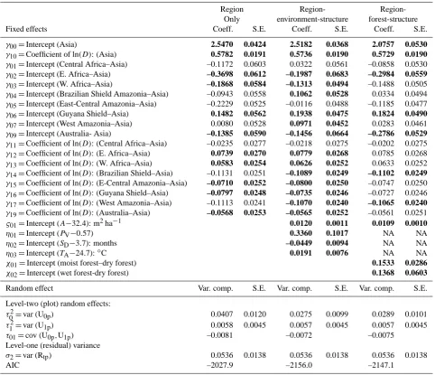
Region Region- Region-Only environment-structure forest-structure Fixed effects Coeff. S.E. Coeff. S.E. Coeff. S.E.
γ00=Intercept (Asia) 2.5470 0.0424 2.5182 0.0368 2.0757 0.0530
γ10=Coefficient of ln(D): (Asia) 0.5782 0.0191 0.5736 0.0190 0.5729 0.0190
γ01=Intercept (Central Africa–Asia) –0.1172 0.0603 0.0322 0.0561 –0.0858 0.0530
γ02=Intercept (E. Africa–Asia) –0.3698 0.0612 –0.1987 0.0683 –0.2984 0.0559
γ03=Intercept (W. Africa–Asia) –0.1868 0.0584 –0.1313 0.0494 –0.1488 0.0505
γ04=Intercept (Brazilian Shield Amazonia–Asia) –0.0943 0.0558 0.1062 0.0528 0.0334 0.0494 γ05=Intercept (East-Central Amazonia–Asia) –0.2229 0.0525 –0.0116 0.0488 –0.1185 0.0477
γ06=Intercept (Guyana Shield–Asia) 0.1482 0.0562 0.1938 0.0475 0.1824 0.0490
γ07=Intercept (West Amazonia–Asia) 0.0080 0.0528 0.0971 0.0452 0.0283 0.0461
γ09=Intercept (Australia- Asia) –0.1385 0.0590 –0.1456 0.0664 –0.2786 0.0529
γ11=Coefficient of ln(D): (Central Africa–Asia) –0.0235 0.0277 –0.0218 0.0275 –0.0202 0.0275
γ12=Coefficient of ln(D): (E. Africa–Asia) 0.0739 0.0270 0.0779 0.0268 0.0785 0.0268
γ13=Coefficient of ln(D): (W. Africa–Asia) 0.0583 0.0254 0.0626 0.0252 0.0633 0.0252
γ14=Coefficient of ln(D): (Brazilian Shield–Asia) –0.1131 0.0251 –0.1089 0.0249 –0.1102 0.0249
γ15=Coefficient of ln(D): (E-Central Amazonia–Asia) –0.0710 0.0252 –0.0800 0.0250 –0.0747 0.0250 γ16=Coefficient of ln(D): (Guyana Shield–Asia) –0.0797 0.0248 –0.0735 0.0246 –0.0727 0.0246
γ17=Coefficient of ln(D): (West Amazonia–Asia) –0.1113 0.0241 –0.1070 0.0240 –0.1065 0.0240
γ19=Coefficient of ln(D): (Australia–Asia) –0.0568 0.0253 –0.0565 0.0252 –0.0561 0.0251
ς01=Intercept (A−32.4): m2ha−1 0.0120 0.0011 0.0109 0.0010
η01=Intercept (PV−0.57) 0.3360 0.1017 NA NA
η02=Intercept (SD−3.7): months –0.0449 0.0094 NA NA
η03=Intercept (TA−24.7):◦C 0.0191 0.0076 NA NA
χ01=Intercept (moist forest–dry forest) 0.1533 0.0286
χ02=Intercept (wet forest-dry forest) 0.1368 0.0603
Random effect Var. comp. S.E. Var. comp. S.E. Var. comp. S.E.
Level-two (plot) random effects:
τ02=var (U0p) 0.0407 0.0120 0.0275 0.0099 0.0289 0.0101
τ12=var (U1p) 0.0058 0.0045 0.0057 0.0045 0.0057 0.0045
τ01=cov (U0p,U1p) –0.0081 –0.0072 –0.0075
Level-one (residual) variance
σ2=var (Rtp) 0.0536 0.0138 0.0536 0.0138 0.0536 0.0138
AIC –2027.9 –2156.0 –2147.1
3.2 Regional-level models
Figure 3 summarizes the tree height data by region, with trees again partitioned according to three size classes (D <2 dm, 2≤D≤4 dm and D >4 dm) and according to the forest moisture classification as described above. This shows that in dry forests the median height of trees in the smallestD
class (1 to 2 dm D) on the Guyana Shield is significantly greater than trees in East and West Africa, on the Brazilian Shield and in Australia. For moist forests, the tallest trees in this size-class were encountered on the Guyana Shield
0 10 20 30 40 50 ab b ab accac ac
0 10 20 30 40 50 c a
bcaba ab cd 0 10 20 30 40 50 c ab d bc d c b a c a d 0 10 20 30 40 50 60 a b c a b d d e e 0 10 20 30 40 50 60 c e a b d
de e e cf
0 10 20 30 40 50 60 a b g a ced d h ef c fg 0 10 20 30 40 50 60 A si a C en tr al A fr ic a E as t A fr ic a W es t A fr ic a A u st ra lia B ra zi li an S h ie ld E as t-C en tr al A m az o n ia G u ya n a S h ie ld W es t A m az o n ia C en tr al A m er ic as a b 0 10 20 30 40 50 60 A si a C en tr al A fr ic a E as t A fr ic a W es t A fr ic a A u st ra li a B ra zi li an S h ie ld E as t-C en tr al A m az o n ia G u ya n a S h ie ld W es t A m az o n ia C en tr al A m er ic as a b a a b
1 dm <D< 2 dm 1 dm <D< 2 dm
1 dm <D< 2 dm
2 dm <D< 4 dm
2 dm <D< 4 dm
2 dm <D< 4 dm
Dry forests
Wet forests
D> 4 dm
D> 4 dm
D> 4 dm
T re e h ei gh t (m ) T re e h ei g h t (m ) T re e h ei gh t (m ) T re e h ei gh t (m ) 0 10 20 30 40 50 60 A si a C en tr al A fr ic a E as t A fr ic a W es t A fr ic a A u st ra li a B ra zi li an S h ie ld E as t-C en tr al A m az o n ia G u ya n a S h ie ld W es t A m az o n ia C en tr al A m er ic as Moist forests
[image:13.595.309.545.63.278.2]D> 4 dm
Fig. 3. Tree height distribution by diameter class and region for
dry, moist, and wet forests. Bars indicate upper and lower 0.05 quantiles. Different letters within each panel indicate significant differences (p <0.05).
Similar to the models that included continent, assigning re-gion as a fixed effect while retaining plot as a random effect also resulted in significant improvement in the model relative to the multilevel model based onDalone, with significant differences among regions and withA, and climate variables also being significant (Table 3). Nevertheless, comparing the AIC and the plot random-effect terms of the continental-level models (Table 2), the overall improvement with this in-creased level of complexity, although significant, was also relatively modest (AIC of−2156 versus −2127), with the coefficients for the structural and environmental parameters hardly changed.
Figure 4 illustrates the ability of the region-environment-structure model to predict stand-level height from diameter measurements. Here we have estimatedH from associated
Don the same tree and then presented each plot’s medianHˆ
so predicted (denoted △
H) against the actual measured median height,H∩. This shows that the region-environment-structure model successfully predictsH∩, except for some of the tallest
0 10 20 30 40
0 1 0 2 0 3 0 4 0
Measured median height (m)
P re d ic te d m ed ia n h ei g h t (m ) S.E. Asia C. Africa E. Africa W. Africa Brazilian Shield E.-C. Amazon Guyana Shield W. Amazon Australia
Fig. 4. Median predicted tree height versus measured tree height by
plot for the region-environment-structure model. The solid red line indicates the 1:1 relationship.
stands on the Guyana Shield where △
His an underestimate of
∩
H. Plots of the model residuals versusA,PV,SDandD, as
well as versus annual precipitation, are presented in the Sup-plement, (Fig. S3). This shows the model to provide a reli-able, unbiased estimate of tree heights across a wide range of environmental conditions and stand basal areas. The ex-plained variance of the region-environment-structure model as quantified by the calculation of a “pseudo”R2gives anR2
for level 1 (within plots) of 0.61 and a level-2 (between-plot)
R2of 0.80.
The modelled relationship between the region-only and region-environment-structure model (the latter with all cen-tered structural/environmental terms set to zero) are shown in Fig. 5a and b, respectively. Figure 5a can be considered to show the differences observed in the average H:D relation-ship for the different regions with Fig. 5b showing the results of subtracting the effects of environment and forest structure from these observed regionally dependent relationships. Fig-ure 5b suggests a broad separation of the nine regions into two fundamental groups. Those with a higherHˆ at any given
[image:13.595.49.285.65.396.2]5 10 15 20
0
20
4
0
6
0
Diameter (dm)
S.E. Asia C. Africa E. Africa W. Africa Brazilian Shield E.-C. Amazon Guyana Shield W. Amazon Australia Pantropical
Diameter (dm)
5 10 15 20
0
20
4
0
6
0
Diameter (dm)
T
re
e
h
ei
gh
t
(m
)
[image:14.595.103.495.62.236.2](a) (b)
Fig. 5. Model predictions showing fitted relationship between tree height (H) and diameterDfor the different regions (a) region-only model;
(b) region-environment-structure model. Also shown in each panel is the associated pantropical model (pantropical only or
pantropical-environment-structure), this showing the relationship betweenH andDfor the dataset as a whole.
3.3 Plot-to-plot variation
Although the estimated 0.8 of the between-plot variance ac-counted for by the regional-environment-structure model is quite high, it was also of interest to evaluate whether the remaining 0.2 could be related to other factors; some as-pect of soil physical and/or chemical properties being the most obvious candidates. Detailed soil data are available for a large number of South American sites sampled as part of the RAINFOR network (Quesada et al., 2010), with addi-tional soil data and soil profile descriptions from some of the sites included in the H:D analyses above having been collected in Australia, Bolivia, Brazil, Brunei, Cameroon, French Guiana, Ghana, Malaysia and Peru over recent years and analyzed with the same methodology.
Although an examination of the relationships between soil chemistry (exchangeable cations, total soil P, soil C/N), soil texture and variability in plot-effect terms revealed no sta-tistically significant relations (p >0.05), robust regression techniques revealed plot intercept terms to be related to the index of soil physical properties developed by Quesada et al. (2010), a measure of effective soil depth, soil structure, topography and anoxia. Fig. 6 shows that the random plot intercept term for both the continent-environment-structure and regional-environment-structure models declines signifi-cantly as5increases, with the relationship being stronger for the former (P <0.001 versusP <0.05 ). Interestingly, many of the lower outliers in the regional-environment-structure model plot (Fig. 6b) were identified as forests existing at the lowest rainfall extremes for their region, generally existing with savanna/forest transition zones.
The random slope intercept, although showing a slight ten-dency to increase with5, showed no overall statistically sig-nificant relationship with 5 for the
regional-environment-structure model and only being significant atP <0.05 for the continent-environment-structure model.
4 Discussion
4.1 Comparison with other models
Based on our preliminary analyses as provided in the Sup-plement, we chose a log(H ):log(D)model for our analysis only after also considering other commonly applied tropical
H:D allometric functions. Such equations included a
combi-nation of log–linear and asymptotic forms of up to three pa-rameters (Bullock, 2000; Thomas, 1996; Bailey, 1980; Fang and Bailey, 1998). Although it has been suggested that log– normal and log–log relationships often do equally well in fit-ting height to diameter, we found that log–normal relation-ships were insufficient for normalizing data and had higher deviation than log–log models.
Cessation of tree height growth in older trees (Kira, 1978) and relatively similar individual tree canopy heights within sites has given rise to calls for the application of asymptotic curve-fitting to model monotonic H:D relationships (Bul-lock, 2000). For individual species, girth continues to in-crease while height remains virtually constant. This height model selection based on biologically meaningful parame-ters such as species maximum height (Hmax) has the
advan-tage of allowing forHmaxcomparisons between species and
for the evaluation of inter-relationships between structural at-tributes and functional groups. For example,Hmaxmay
y =0.113 0.0202- x
-0.5 -0.4 -0.3 -0.2 -0.1 0.0 0.1 0.2 0.3 0.4 0.5
In
te
rc
ep
t
,
lo
g
(m
)
0 2 4 6 8 10 Quesada Index
-0.5 -0.4 -0.3 -0.2 -0.1 0.0 0.1 0.2 0.3 0.4 0.5
In
te
rc
ep
t
,
lo
g
(m
)
0 2 4 6 8 10 Quesada Index
Central Africa West Africa S.E. Asia
Australia Brazilian Shield C.E. Amazon
Western Amazon Guyana Shield Column 36 Transitional forests
[image:15.595.129.465.63.276.2](a) (b)
Fig. 6. Relationship between plot-level intercept residual terms and the Quesada et al. (2010) index of soil physical properties (a)
pantropical-environment-structure model; (b) regional-pantropical-environment-structure model.
and Poorter et al. (2006) found that approximately one-fourth of the species examined in a Bolivian forest failed to exhibit asymptotic H:D relationships. In those species exhibiting asymptotic relations it is unclear whether the reduction in tree height growth with height in mature stands represents the approach to critical maximum height, or alternatively, the response of tall trees attaining a canopy position and reduced competition for light (King, 1990). In any case, because of the wide variation observed in individual species H:D rela-tionships (Poorter et al., 2006), and because of inter-species variations in Hmax (Baker et al., 2009), it is unlikely that
any single meaningful asymptotic relationship will apply for a typically diverse tropical forest stand. It is probably for this reason that, at the plot level, we found that the asymp-totic function failed to consistently converge for dry and wet forests, and that this function grossly overestimated height in many of our forests when the function did converge.
When our pantropical closed-canopy dry and moist for-est models are compared to the second most comprehensive pantropical data set (Brown et al., 1989), that being based on 3824 tree measurements, a strikingly close correspondence was indicated between the slope coefficients of the two equa-tions. Although such small differences could be taken to in-dicate a robust H:D relationship at the pantropical level, thus supporting the theory of a universal H:D scaling relationship (e.g., Niklas and Spatz, 2004), differences in tree architec-ture become apparent when the Brown moist model is com-pared to our region-specific models. The Brown moist mod-els only estimateH to within−22% to+4% of the median of measured values. This is a substantial bias compared to our more sophisticated models that include environment and
forest structure to accurately estimate H (Supplement, Ta-ble S3, Fig. S2). Moreover, as shown in TaTa-ble 3, Fig. 5 and discussed further below, significant differences in the H:D scaling exponent also exist for the different tropical regions, even once these variations in stand structure and environment are taken into account.
4.2 Plot-to-plot variations
It has been demonstrated that trees exhibit variations in ar-chitectural properties, both within and across sites (Nogueira et al., 2008b; Sterck and Bongers, 2001; O’Brien et al., 1995; Osunkoya et al., 2007; Poorter et al., 2003, 2006). The pantropical tree architecture dataset presented here rep-resents a first step towards unifying our understanding of global tree architecture data. Our aim here was to examine whether and how forest structure, geography and climate in-teract to affect tropical tree H:D allometric relationships. We have found significant differences in H:D allometries at con-tinental and regional scales as well as detecting significant effects of climate and forest structure.
As trees grow taller and crowns extend laterally, trees necessarily invest in stem diameter growth to support large crowns, replace functionally inactive vessels, and resist the increased wind stress. Although interpretable as giving rise to asymptotic H:D relationships (Sterck et al., 2005), this phenomenon can also be viewed in terms of the allometric scaling coefficient (β1) in Eq. (1) necessarily being less than
both in meters) should apply. This relates toH=20.2D0.67
in the form and units of the current model and from the calcu-lations associated with the pantropical model in Sect 3.1.2 it appears that some trees found atD=1 dm were approaching heights only just less than their buckling limit and also that some plots have allometric scaling coefficients very close to the theoretical 0.67 maximum (King et al., 2009). Neverthe-less, as the slope and intercept of the plot random effect terms were negatively correlated, it seems unlikely for both to oc-cur simultaneously. Rather, it would seem that in plots where trees tend to be close to their buckling limit at D=1 dm they subsequently grow with allometric scaling coefficients considerably below the theoretical 0.67 limit, thus assum-ing a greater safety margin as they grow taller. This is not surprising as light competition and hence premium on ver-tical growth, is most severe at lower levels, while daytime wind speeds, and hence the risk of direct mechanical dam-age, may increase more-or-less exponentially with canopy height (Kruijt et al., 2000).
Overall, structural and environmental effects on H:D al-lometry observed were expressed as changes in the intercept rather than in the slope of the log–log models (Tables 2 and 3). Since the intercept in our model has a meaningful in-terpretation (being the natural logarithm of the height of the average tree atD=1 dm), this means that effects of envi-ronment on forest tree H are already evident at the late-sapling stage with the scaling coefficient for all regions, stand structures and environmental conditions below the theoreti-cal buckling limit mentioned above.
4.3 Vegetation structure effects
We found stand basal area(A), but not stem density, to be an important driver of variation in H:D allometry. All else being equal, forests with a greaterAtended to have taller trees at any givenD. As high stem densities can occur even in forests with lower stature and lower biomass, the stronger effect of
Acan probably be explained in terms of greater competition for light imposed by high basal area stands, this necessitat-ing the allocation of more resources to height versus diameter growth, thereby allowing trees to reach the upper layers more rapidly once gaps are formed and to increase their chance of survival. This supports findings from two old-growth forests in Malaysia which have differingAand corresponding dif-ferent H:D allometry, suggesting a general trend (King et al., 2009). King (1981) also cites data from Ek (1974) show-ing that widely spaced trees growshow-ing in open environments have thicker trunks than those of forest-grown trees of sim-ilar height; and, working with a Cordia alliodora plantation spacing trial in Costa Rica, Hummel (2000) found that trees that were more widely spaced tended to have a greater D
than those that were more closely packed, but with no effect of stem density onH. She interpreted this result in terms of classic plant population biology size-density theory (Yoda et al., 1963) as applied to commercial forestry management
operations (Drew and Flewelling, 1977). Here it is consid-ered that trees of a given age will generally all be of a sim-ilar height but with a lower average basal area (at any given age/height) when growing in a denser stand due to lower rates of light interception per tree. More densely packed stems may also benefit from wind-sheltering allowing stems to put fewer resources into diameter increment for stability; the ef-fects of light and wind-sheltering are thus difficult to separate (Henry and Aarssen, 1999).
4.4 Climatic effects
Results from the pantropical structure environment model provide strong evidence for environmental effects on tree
H:D relationships, which persisted even after continental or
regional location were taken into account. Precipitation co-efficient of variance (PV), numbers of months with<0.1 m
of rainfall (SD) and temperature (TA) were all highly
signifi-cant. It should also be noted that altitude (AL) andTAwere
strongly correlated; inclusion of one of these variables in the model negated the other. In all cases, environment was found to affect the intercept, but not the slope, of the H:D relation-ship.
4.4.1 Temporal distribution of rainfall
Dry-season length emerged as one key factor influencing
H:D relationships, with a longer dry season being associated
with stouter trees (Tables 2 and 3). The magnitude of this effect can be appreciated from the data underlying Fig. 7b, for whichPV=0.56 in all cases (close to the dataset
aver-age value), then calculating Hˆ withAandTA also at their
overall dataset average values. Applying Eq. (13) then for
D=1 dm, then we obtainHˆ =13.0 m forSD=3 months (as
for Cavalla, Liberia). On the other hand, forSD=9 months
(as for Tucavaca, Bolivia) we estimate forH only 8.9 m. For
D=5 dm, there is a difference inHˆ of nearly 10 m with
ˆ
H=20.9 m versus 30.5 m forSD=9 versus 3 months,
re-spectively. Dry season length thus exerts a strong effect on tropical forest tree H:D allometry.