City, University of London Institutional Repository
Citation
:
Alessandretti, L., ElBahrawy, A., Aiello, L. M. and Baronchelli, A. ORCID:
0000-0002-0255-0829 (2018). Machine Learning the Cryptocurrency Market. Complexity, 2018,
doi: 10.1155/2018/8983590
This is the accepted version of the paper.
This version of the publication may differ from the final published
version.
Permanent repository link: http://openaccess.city.ac.uk/19829/
Link to published version
:
http://dx.doi.org/10.1155/2018/8983590
Copyright and reuse:
City Research Online aims to make research
outputs of City, University of London available to a wider audience.
Copyright and Moral Rights remain with the author(s) and/or copyright
holders. URLs from City Research Online may be freely distributed and
linked to.
City Research Online:
http://openaccess.city.ac.uk/
[email protected]
Research Article
Anticipating Cryptocurrency Prices Using Machine Learning
Laura Alessandretti ,
1Abeer ElBahrawy ,
2Luca Maria Aiello ,
3and Andrea Baronchelli
2,41Technical University of Denmark, 2800 Kgs. Lyngby, Denmark
2City, University of London, Department of Mathematics, London EC1V 0HB, UK
3Nokia Bell Labs, Cambridge CB3 0FA, UK
4UCL Centre for Blockchain Technologies, University College London, UK
Correspondence should be addressed to Andrea Baronchelli; [email protected]
Received 29 May 2018; Revised 28 September 2018; Accepted 17 October 2018; Published 4 November 2018
Academic Editor: Massimiliano Zanin
Copyright © 2018 Laura Alessandretti et al. This is an open access article distributed under the Creative Commons Attribution License, which permits unrestricted use, distribution, and reproduction in any medium, provided the original work is properly cited.
Machine learning and AI-assisted trading have attracted growing interest for the past few years. Here, we use this approach to test the hypothesis that the inefficiency of the cryptocurrency market can be exploited to generate abnormal profits. We analyse daily data for1, 681cryptocurrencies for the period between Nov. 2015 and Apr. 2018. We show that simple trading strategies assisted by state-of-the-art machine learning algorithms outperform standard benchmarks. Our results show that nontrivial, but ultimately simple, algorithmic mechanisms can help anticipate the short-term evolution of the cryptocurrency market.
1. Introduction
The popularity of cryptocurrencies has skyrocketed in 2017 due to several consecutive months of superexponential growth of their market capitalization [1], which peaked at more than $800 billions in Jan. 2018. Today, there are more than1, 500actively traded cryptocurrencies. Between2.9and 5.8millions of private as well as institutional investors are in the different transaction networks, according to a recent survey [2], and access to the market has become easier over time. Major cryptocurrencies can be bought using fiat currency in a number of online exchanges (e.g., Binance [3], Upbit [4], Kraken [5], etc.) and then be used in their turn to buy less popular cryptocurrencies. The volume of daily exchanges is currently superior to $15 billions. Since 2017, over 170 hedge funds specialised in cryptocurrencies have emerged and Bitcoin futures have been launched to address institutional demand for trading and hedging Bitcoin [6].
The market is diverse and provides investors with many different products. Just to mention a few, Bitcoin was expressly designed as a medium of exchange [7, 8]; Dash offers improved services on top of Bitcoin’s feature set, includ-ing instantaneous and private transactions [9]; Ethereum is
a public, blockchain-based distributed computing platform featuring smart contract (scripting) functionality, and Ether is a cryptocurrency whose blockchain is generated by the Ethereum platform [10]; Ripple is a real-time gross settlement system (RTGS), currency exchange, and remittance network Ripple [11], and IOTA is focused on providing secure com-munications and payments between agents on the Internet of Things [12].
The emergence of a self-organised market of virtual currencies and/or assets whose value is generated primarily by social consensus [13] has naturally attracted interest from the scientific community [8, 14–30]. Recent results have shown that the long-term properties of the cryptocurrency marked have remained stable between 2013 and 2017 and are compatible with a scenario in which investors simply sample the market and allocate their money according to the cryptocurrency’s market shares [1]. While this is true on average, various studies have focused on the analysis and forecasting of price fluctuations, using mostly traditional approaches for financial markets analysis and prediction [31– 35].
The success of machine learning techniques for stock markets prediction [36–42] suggests that these methods
could be effective also in predicting cryptocurrencies prices. However, the application of machine learning algorithms to the cryptocurrency market has been limited so far to the analysis of Bitcoin prices, using random forests [43], Bayesian neural network [44], long short-term memory neural net-work [45], and other algorithms [32, 46]. These studies were able to anticipate, to different degrees, the price fluctuations of Bitcoin, and revealed that best results were achieved by neural network based algorithms. Deep reinforcement learning was showed to beat the uniform buy and hold strategy [47] in predicting the prices of 12 cryptocurrencies over one-year period [48].
Other attempts to use machine learning to predict the prices of cryptocurrencies other than Bitcoin come from nonacademic sources [49–54]. Most of these analyses focused on a limited number of currencies and did not provide benchmark comparisons for their results.
Here, we test the performance of three models in predict-ing daily cryptocurrency price for 1,681 currencies. Two of the models are based on gradient boosting decision trees [55] and one is based on long short-term memory (LSTM) recurrent neural networks [56]. In all cases, we build investment portfolios based on the predictions and we compare their performance in terms of return on investment. We find that all of the three models perform better than a baseline ‘simple moving average’ model [57–60] where a currency’s price is predicted as the average price across the preceding days and that the method based on long short-term memory recurrent neural networks systematically yields the best return on investment.
The article is structured as follows: In Materials and Methods we describe the data (see Data Description and Preprocessing), the metrics characterizing cryptocurrencies that are used along the paper (see Metrics), the forecasting algorithms (see Forecasting Algorithms), and the evaluation metrics (see Evaluation). In Results, we present and compare the results obtained with the three forecasting algorithms and the baseline method. In Conclusion, we conclude and discuss results.
2. Materials and Methods
2.1. Data Description and Preprocessing. Cryptocurrency data was extracted from the website Coin Market Cap [61], collecting daily data from 300 exchange markets platforms starting in the period between November 11, 2015, and April 24, 2018. The dataset contains the daily price in US dollars, the market capitalization, and the trading volume of 1, 681cryptocurrencies, where the market capitalization is the product between price and circulating supply, and the volume is the number of coins exchanged in a day. The daily price is computed as the volume weighted average of all prices reported at each market. Figure 1 shows the number of currencies with trading volume larger than𝑉𝑚𝑖𝑛over time, for different values of𝑉𝑚𝑖𝑛. In the following sections, we consider that only currencies with daily trading volume higher than 105 USD (United States dollar) can be traded at any given day.
cr
yp
to
cur
rencies
103
102 101
100
Ja
n 16
M
ay 16
S
ep 16 Jan 17
M
ay 17
S
ep 17 Jan 18
6GCH= $0
6GCH= $1000
6GCH= $10000
6GCH= $100000
Figure 1:Number of cryptocurrencies.The cryptocurrencies with volume higher than𝑉𝑚𝑖𝑛as a function of time, for different values of 𝑉𝑚𝑖𝑛. For visualization purposes, curves are averaged over a rolling
window of10days.
The website lists cryptocurrencies traded on public exchange markets that have existed for more than 30 days and for which an API and a public URL showing the total mined supply are available. Information on the market capitalization of cryptocurrencies that are not traded in the 6 hours preceding the weekly release of data is not included on the website. Cryptocurrencies inactive for 7 days are not included in the list released. These measures imply that some cryptocurrencies can disappear from the list to reappear later on. In this case, we consider the price to be the same as before disappearing. However, this choice does not affect results since only in 28 cases the currency has volume higher than 105USD right before disappearing (note that there are 124,328 entries in the dataset with volume larger than105USD).
2.2. Metrics. Cryptocurrencies are characterized over time by several metrics, namely,
(i) Price, the exchange rate, determined by supply and demand dynamics.
(ii) Market capitalization, the product of the circulating supply and the price.
(iii) Market share, the market capitalization of a currency normalized by the total market capitalization.
(iv) Rank, the rank of currency based on its market capitalization.
(v) Volume, coins traded in the last 24 hours.
(vi) Age, lifetime of the currency in days.
The profitability of a currency𝑐over time can be quanti-fied through thereturn on investment (ROI), measuring the return of an investment made at day𝑡𝑖 relative to the cost [62]. The index𝑖rolls across days and it is included between 0 and 895, with𝑡0 =November 11, 2015, and𝑡895 =April 24, 2018. Since we are interested in the short-term performance, we consider the return on investment after 1 day defined as
𝑅𝑂𝐼 (𝑐, 𝑡𝑖) = 𝑝𝑟𝑖𝑐𝑒 (𝑐, 𝑡𝑖) − 𝑝𝑟𝑖𝑐𝑒 (𝑐, 𝑡𝑖− 1)
Jan 16 May 16 Sep 16 Jan 17 May 17 Sep 17 Jan 18 day
0.00 0.05 0.10 0.15 0.20
roi
mean=0.011
Bitcoin mean=0.005
−0.05
[image:4.600.180.418.72.180.2]cryptos with volume>105
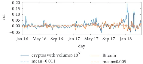
Figure 2:Return on investment over time.The daily return on investment for Bitcoin (orange line) and the average for currencies with volume larger than𝑉𝑚𝑖𝑛= 105USD (blue line). Their average value across time (dashed lines) is larger than0. For visualization purposes, curves are averaged over a rolling window of10days.
#.
#D
#1
Features
Features
Features
Features
Features
Features
Features
Features
Features
Features
Features
Features T
T
T T
T
T T
T
T T
T T
w w w w
Training Test
NC− 7NL;CHCHA NC− 7NL;CHCHA+ 1 ND NC− 1 NC
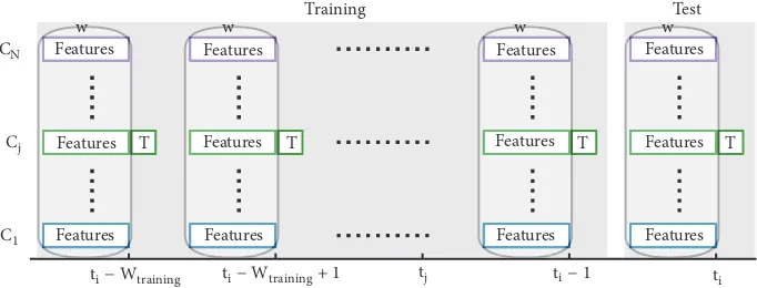
Figure 3:Schematic description of Method 1.The training set is composed of features and target (T) pairs, where features are various characteristics of a currency𝑐𝑖, computed across the𝑤days preceding time𝑡𝑗and the target𝑇is the price of𝑐𝑖at𝑡𝑗. The features-target pairs are computed for all currencies𝑐𝑖and all values of𝑡𝑗included between𝑡𝑖− 𝑊𝑡𝑟𝑎𝑖𝑛𝑖𝑛𝑔and𝑡𝑖− 1. The test set includes features-target pairs for all currencies with trading volume larger than105USD at𝑡𝑖, where the target is the price at time𝑡𝑖and features are computed in the𝑤days preceding𝑡𝑖.
In Figure 2, we show the evolution of the𝑅𝑂𝐼over time for Bitcoin (orange line) and on average for currencies whose volume is larger than𝑉𝑚𝑖𝑛= 105USD at𝑡𝑖− 1(blue line). In both cases, the average return on investment over the period considered is larger than 0, reflecting the overall growth of the market.
2.3. Forecasting Algorithms. We test and compare three supervised methods for short-term price forecasting. The first two methods rely on XGBoost [63], an open-source scalable machine learning system for tree boosting used in a number of winning Kaggle solutions (17/29 in 2015) [64]. The third method is based on the long short-term memory (LSTM) algorithm for recurrent neural networks [56] that have demonstrated to achieve state-of-the-art results in time-series forecasting [65].
Method 1. The first method considers one single regression model to describe the change in price of all currencies (see Figure 3). The model is an ensemble of regression trees built by the XGBoost algorithm. The features of the model are characteristics of a currency between time𝑡𝑗−𝑤and𝑡𝑗−1and the target is the ROI of the currency at time𝑡𝑗, where𝑤is a parameter to be determined. The characteristics considered for each currency are price, market capitalization, market
share, rank, volume, and ROI (see (1)). The features for the regression are built across the window between𝑡𝑗−𝑤and𝑡𝑗−1 included (see Figure 3). Specifically, we consider the average, the standard deviation, the median, the last value, and the trend (e.g., the difference between last and first value) of the properties listed above. In the training phase, we include all currencies with volume larger than105USD and𝑡𝑗between 𝑡𝑖−𝑊𝑡𝑟𝑎𝑖𝑛𝑖𝑛𝑔and𝑡𝑖. In general, larger training windows do not necessarily lead to better results (see results section), because the market evolves across time. In the prediction phase, we test on the set of existing currencies at day𝑡𝑖. This procedure is repeated for values of𝑡𝑖included between January 1, 2016, and April 24, 2018.
[image:4.600.129.469.243.371.2]#.
#D
#1
Features
Features
Features
T Features
Features
Features
T Features
Features
Features
T Features
Features
Features T w w
w w
Training Test
[image:5.600.129.470.73.203.2]NC− 7NL;CHCHA NC− 7NL;CHCHA+ 1 ND NC− 1 NC
Figure 4:Schematic description of Method 2.The training set is composed of features and target (T) pairs, where features are various characteristics of all currencies, computed across the𝑤days preceding time𝑡𝑗and the target𝑇is the price of𝑐𝑖at𝑡𝑗. The features-target pairs include a single currency𝑐𝑖, for all values of𝑡𝑗included between𝑡𝑖− 𝑊𝑡𝑟𝑎𝑖𝑛𝑖𝑛𝑔and𝑡𝑖− 1. The test set contains a single features-target pair: the characteristics of all currencies, computed across the𝑤days preceding time𝑡𝑖and the price of𝑐𝑖at𝑡𝑖.
quantities: price, market capitalization, market share, rank, volume, and ROI) across a window of length𝑤. The model for currency𝑐𝑖is trained with pairs features target between times𝑡𝑖− 𝑊𝑡𝑟𝑎𝑖𝑛𝑖𝑛𝑔and𝑡𝑖− 1. The prediction set includes only one pair: the features (computed between𝑡𝑖− 𝑤and𝑡𝑖− 1) and the target (computed at𝑡𝑖) of currency𝑐𝑖.
Method 3. The third method is based on long short-term memory networks, a special kind of recurrent neural net-works, capable of learning long-term dependencies. As for Method 2, we build a different model for each currency. Each model predicts the ROI of a given currency at day𝑡𝑖based on the values of the ROI of the same currency between days 𝑡𝑖− 𝑤and𝑡𝑖− 1included.
Baseline Method. As baseline method, we adopt the simple moving average strategy (SMA) widely tested and used as a null model in stock market prediction [57–60]. It estimates the price of a currency at day𝑡𝑖 as the average price of the same currency between𝑡𝑖− 𝑤and𝑡𝑖− 1included.
2.4. Evaluation. We compare the performance of various investment portfolios built based on the algorithms predic-tions. The investment portfolio is built at time 𝑡𝑖 − 1 by equally splitting an initial capital among the top𝑛currencies predicted with positive return. Hence, the total return at time 𝑡𝑖is
𝑅 (𝑡𝑖) = 1 𝑛 𝑛 ∑ 𝑐=1
𝑅𝑂𝐼 (𝑐, 𝑡𝑖) . (2)
The portfolios performance is evaluated by computing the Sharpe ratio and the geometric mean return. The Sharpe ratio is defined as
𝑆 (𝑡𝑖) = 𝑠𝑅 𝑅,
(3)
where 𝑅 is the average return on investment obtained between times 0 and𝑡𝑖and𝑠𝑅is the corresponding standard deviation.
The geometric mean return is defined as
𝐺 (𝑡𝑖) =√𝑇
𝑡𝑖 ∏ 𝑡𝑗=1
1 + 𝑅 (𝑡𝑗), (4)
where𝑡𝑖corresponds to the total number of days considered. The cumulative return obtained at 𝑡𝑖 after investing and selling on the following day for the whole period is defined as𝐺(𝑡𝑖)2.
The number of currencies 𝑛to include in a portfolio is chosen at𝑡𝑖by optimising either the geometric mean𝐺(𝑡𝑖−1) (geometric mean optimisation) or the Sharpe ratio𝑆(𝑡𝑖− 1) (Sharpe ratio optimisation) over the possible choices of𝑛. The same approach is used to choose the parameters of Method 1 (𝑤and𝑊𝑡𝑟𝑎𝑖𝑛𝑖𝑛𝑔), Method 2 (𝑤and𝑊𝑡𝑟𝑎𝑖𝑛𝑖𝑛𝑔), and the baseline method (𝑤).
3. Results
We predict the price of the currencies at day 𝑡𝑖, for all 𝑡𝑖 included between Jan 1, 2016, and Apr 24, 2018. The analysis considers all currencies whose age is larger than 50 days since their first appearance and whose volume is larger than $100000. To discount for the effect of the overall market movement (i.e., market growth, for most of the considered period), we consider cryptocurrencies prices expressed in BTC (Bitcoin). This implies that Bitcoin is excluded from our analysis.
3.1. Parameter Setting. First, we choose the parameters for each method. Parameters include the number of currencies 𝑛to include the portfolio as well as the parameters specific to each method. In most cases, at each day𝑡𝑖we choose the parameters that maximise either the geometric mean𝐺(𝑡𝑖−1) (geometric mean optimisation) or the Sharpe ratio𝑆(𝑡𝑖− 1) (Sharpe ratio optimisation) computed between times 0 and 𝑡𝑖.
May 16
Nov 16
May 17
Nov 17
May 18
cu
m
ula
ti
ve
r
et
u
rn
geometric mean optimization
Baseline Method 1
Method 2 Method 3
109
106
103
100
(a)
May 16
Nov 16
May 17
Nov 17
May 18
cu
m
ula
ti
ve
r
et
u
rn
Sharpe ratio optimization
Baseline Method 1
Method 2 Method 3
109
106
103
100
(b)
Figure 5:Cumulative returns.The cumulative returns obtained under the Sharpe ratio optimisation (a) and the geometric mean optimisation (b) for the baseline (blue line), Method 1 (orange line), Method 2 (green line), and Method 3 (red line). Analyses are performed considering prices in BTC.
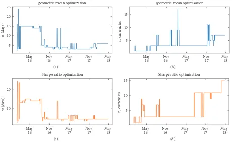
requirement for the𝑅𝑂𝐼to be different from 0) and𝑤 < 30. We find that the value of𝑤mazimising the geometric mean return (see Appendix Section A) and the Sharpe ratio (see Appendix Section A) fluctuates especially before November 2016 and has median value 4 in both cases. The number of currencies included in the portfolio oscillates between 1 and 11 with median at 3, both for the Sharpe ratio (see Appendix Section A) and the geometric mean return (see Appendix Section A) optimisation.
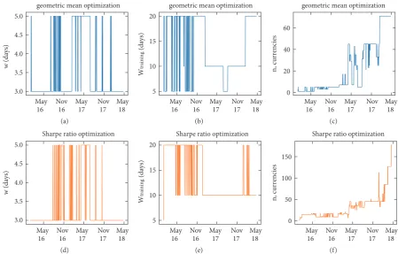
Method 1. We explore values of the window𝑤in{3, 5, 7, 10} days and the training period𝑊𝑡𝑟𝑎𝑖𝑛𝑖𝑛𝑔in{5, 10, 20}days (see Appendix Section A). We find that the median value of the selected window𝑤across time is 7 for both the Sharpe ratio and the geometric mean optimisation. The median value of𝑊𝑡𝑟𝑎𝑖𝑛𝑖𝑛𝑔 is 5 under geometric mean optimisation and 10 under Sharpe ratio optimisation. The number of currencies included in the portfolio oscillates between 1 and 43 with median at 15 for the Sharpe ratio (see Appendix Section A) and 9 for the geometric mean return (see Appendix Section A) optimisation.
Method 2. We explore values of the window𝑤in{3, 5, 7, 10} days and the training period 𝑊𝑡𝑟𝑎𝑖𝑛𝑖𝑛𝑔 in {5, 10, 20} days (see Appendix, Figure 10). The median value of the selected window𝑤across time is 3 for both the Sharpe ratio and the geometric mean optimisation. The median value of𝑊𝑡𝑟𝑎𝑖𝑛𝑖𝑛𝑔 is 10 under geometric mean and Sharpe ratio optimisation. The number of currencies included has median at 17 for the Sharpe ratio and 7 for the geometric mean optimisation (see Appendix Section A).
Method 3. The LSTM has three parameters: The number of epochs, or complete passes through the dataset during the training phase; the number of neurons in the neural network, and the length of the window 𝑤. These parameters are chosen by optimising the price prediction of three currencies (Bitcoin, Ripple, and Ethereum) that have on average the
largest market share across time (excluding Bitcoin Cash that is a fork of Bitcoin). Results (see Appendix Section A) reveal that, in the range of parameters explored, the best results are achieved for𝑤 = 50. Results are not particularly affected by the choice of the number of neurones nor the number of epochs. We choose 1 neuron and 1000 epochs since the larger these two parameters, the larger the computational time. The number of currencies to include in the portfolio is optimised over time by mazimising the geometric mean return (see Appendix Section A) and the Sharpe ratio (see Appendix Section A). In both cases the median number of currencies included is 1.
03- 2016 06- 2016 09- 2016 12- 2016 03- 2017 06- 2017 09- 2017 12- 2017 03- 2018
end
Baseline
(a) (b)
(c) (d)
03- 2016 06- 2016 09- 2016 12- 2016 03- 2017 06- 2017 09- 2017 12- 2017 03- 2018
end
03- 2016
06- 2016
09- 2016
12- 2016
03- 2017
06- 2017
09- 2017
12- 2017
03- 2018
st
ar
t
Method 1
Method 2
03- 2016
06- 2016
09- 2016
12- 2016
03- 2017
06- 2017
09- 2017
12- 2017
03- 2018
st
ar
t
Method 3
−1 −0.1 −0.01 0 0.01 0.1 1
[image:7.600.92.510.70.561.2]G-1
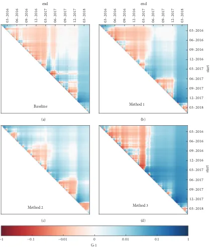
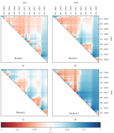
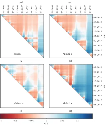
Figure 6:Geometric mean return obtained within different periods of time.The geometric mean return computed between time “start” and “end” using the Sharpe ratio optimisation for the baseline (a), Method 1 (b), Method 2 (c), and Method 3 (d). Note that, for visualization purposes, the figure shows the translated geometric mean return G-1. Shades of red refer to negative returns and shades of blue to positive ones (see colour bar).
gains also when fees up to1% are considered (see Appendix Section C).
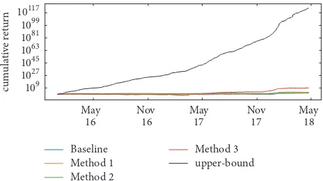
The cumulative return in Figure 5 is obtained by investing between January 1st, 2016 and April 24th, 2018. We investigate the overall performance of the various methods by looking at the geometric mean return obtained in different periods (see Figure 6). Results presented in Figure 6 are obtained under Sharpe ratio optimisation for the baseline (Figure 6(a)), Method 1 (Figure 6(b)), Method 2
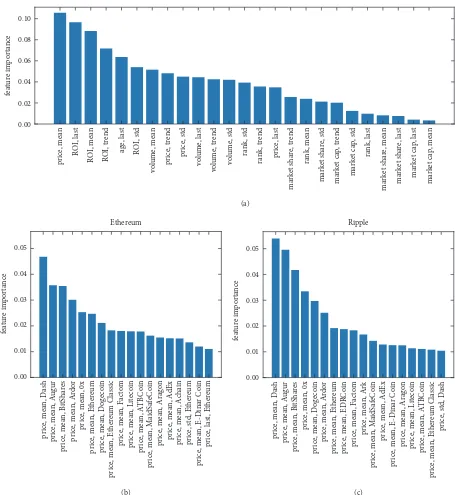
p rice , me an R O I, las t R O I, me an R O I, tr end age, l ast R O I, st d vol u me, me an p rice , tr end p rice , st d volu me, l ast vo lume , tr end vo lu me , st d ra nk, st d ra nk, tr end p rice , last ma rk et sha re , tr end ra nk, me an ma rk et sha re , s td ma rk et ca p , tr end ma rk et ca p , st d ra nk, last market shar e, me an market shar e, l ast ma rk et ca p , last ma rk et ca p , me an 0.00 0.02 0.04 0.06 0.08 0.10 fe at ur e im p o rt an ce p rice , me an, D ash p rice , me an, A ugur p rice , me an, B itS ha re s p rice , me an, Ar do r p rice , me an, 0x p rice , me an, E ther eum p rice , me an, D o ge co in p rice , me an, E ther eum Classic p rice , me an, F ac to m p rice , me an, L it eco in p rice , me an, A T B C o in p rice , me an, M aidSa fe C o in p rice , me an, Arag o n p rice , me an, A dEx p rice , me an, A cha in p rice , s td , E ther eum p rice , me an, E-Dina r C o in p rice
, last, E
[image:8.600.72.527.67.562.2]ther eum 0.00 0.01 0.02 0.03 0.04 0.05 fe at ur e im p o rt an ce Ethereum 0.00 0.01 0.02 0.03 0.04 0.05 p rice , me an, D ash p rice , me an , A u gur p rice , me an , B itS ha re s p rice , me an, 0x p rice , me an, D o ge co in p rice , me an, Ar do r p rice , me an, E ther eum p rice , me an, ED R C o in p rice , me an, F ac to m p rice , me an, Ark p rice , me an, M aidSa fe C o in p rice , me an, A dEx p rice , me an, E-Dina r C o in p rice , me an, Arag o n p rice , me an, L it eco in p rice , me an, A T B C o in p rice , me an, E ther eum Classic pr ic e, s td , D as h fe at ur e im p o rt an ce Ripple (a) (b) (c)
Figure 7:Feature importance for Methods 1 and 2.(a) The average importance of each feature for the XGBoost regression model of Method 1. Results are shown for𝑤 = 7and𝑊𝑡𝑟𝑎𝑖𝑛𝑖𝑛𝑔= 10. (b, c) Examples of average feature importance for the XGBoost regression model developed in Method 2. Results are shown for𝑤 = 3,𝑊𝑡𝑟𝑎𝑖𝑛𝑖𝑛𝑔= 10, for Ethereum (b) and Ripple (c). For visualization purposes, we show only the top features.
3.3. Feature Importance. In Figure 7, we illustrate the relative importance of the various features in Method 1 and Method 2. For Method 1, we show the average feature importance. For Method 2, we show the average feature importance for two sample currencies: Ethereum and Ripple.
3.4. Portfolio Composition. The 10 most selected currencies under Sharpe ratio optimisation are the following:
Baseline. Factom (91 days), E-Dinar Coin (89 days), Ripple (76 days), Ethereum (71 days), Steem (70 days), Lisk (70 days), MaidSafeCoin (69 days), Monero (58 days), BitShares (55 days), EDRCoin (52 days).
Method 2. Ethereum (63 days), Monero (61 days), Factom (51 days), Ripple (42 days), Dash (40 days), Maid Safe Coin (40 days), Siacoin (30 days), NEM (26 days), NXT (26 days), Steem (23 days).
Method 3. Factom (48 days), Monero (46 days), Ethereum (39 days), Lisk (36 days), Maid Safe Coin (32 days), E-Dinar Coin (32 days), BitShares (26 days), B3 Coin (26 days), Dash (25 days), Cryptonite (22 days).
4. Conclusion
We tested the performance of three forecasting models on daily cryptocurrency prices for 1, 681 currencies. Two of them (Method 1 and Method 2) were based on gradient boosting decision trees and one is based on long short-term memory recurrent neural networks (Method 3). In Method 1, the same model was used to predict the return on investment of all currencies; in Method 2, we built a different model for each currency that uses information on the behaviour of the whole market to make a prediction on that single currency; in Method 3, we used a different model for each currency, where the prediction is based on previous prices of the curren-cy.
We built investment portfolios based on the predictions of the different method and compared their performance with that of a baseline represented by the well-known simple moving average strategy. The parameters of each model were optimised for all but Method 3 on a daily basis, based on the outcome of each parameters choice in previous times. We used two evaluation metrics used for parameter optimisation: The geometric mean return and the Sharpe ratio. To discount the effect of the overall market growth, cryptocurrencies prices were expressed in Bitcoin. All strategies produced profit (expressed in Bitcoin) over the entire considered period and for a large set of shorter trading periods (different combinations of start and end dates for the trading activ-ity), also when transaction fees up to 0.2% are consid-ered.
The three methods performed better than the baseline strategy when the investment strategy was ran over the whole period considered. The optimisation of parameters based on the Sharpe ratio achieved larger returns. Methods based on gradient boosting decision trees (Methods 1 and 2) worked best when predictions were based on short-term windows of 5/10 days, suggesting they exploit well mostly short-term dependencies. Instead, LSTM recurrent neural networks worked best when predictions were based on ∼ 50 days of data, since they are able to capture also long-term dependencies and are very stable against price volatility. They allowed making profit also if transaction fees up to 1% are considered. Methods based on gradient boosting decision trees allow better interpreting results. We found that the prices and the returns of a currency in the last few days preceding the prediction were leading factors to anticipate its behaviour. Among the two methods based on random forests, the one considering a different model for each currency performed best (Method 2). Finally, it is worth noting that the three methods proposed perform better when
predictions are based on prices in Bitcoin rather than prices in USD. This suggests that forecasting simultaneously the overall cryptocurrency market trend and the developments of individual currencies is more challenging than forecasting the latter alone.
It is important to stress that our study has limitations. First, we did not attempt to exploit the existence of dif-ferent prices on difdif-ferent exchanges, the consideration of which could open the way to significantly higher returns on investment. Second, we ignored intraday price fluctuations and considered an average daily price. Finally, and crucially, we run a theoretical test in which the available supply of Bitcoin is unlimited and none of our trades influence the market. Notwithstanding these simplifying assumptions, the methods we presented were systematically and consistently able to identify outperforming currencies. Extending the current analysis by considering these and other elements of the market is a direction for future work.
A different yet promising approach to the study cryp-tocurrencies consists in quantifying the impact of public opinion, as measured through social media traces, on the market behaviour, in the same spirit in which this was done for the stock market [67]. While it was shown that social media traces can be also effective predictors of Bitcoin [68–74] and other currencies [75] price fluctuations, our knowledge of their effects on the whole cryptocurrency market remain limited and is an interesting direction for future work.
Appendix
A. Parameter Optimisation
In Figure 8, we show the optimisation of the parameters𝑤 (a, c) and𝑛(b, d) for the baseline strategy. In Figure 9, we show the optimisation of the parameters𝑤(a, d),𝑊𝑡𝑟𝑎𝑖𝑛𝑖𝑛𝑔 (b, e), and𝑛(c, f) for Method 1. In Figure 10, we show the optimisation of the parameters𝑤(a, d),𝑊𝑡𝑟𝑎𝑖𝑛𝑖𝑛𝑔 (b, e), and 𝑛 (c, f) for Method 2. In Figure 11, we show the median squared error obtained under different training window choices (a), number of epochs (b) and number of neurons (c), for Ethereum, Bitcoin and Ripple. In Figure 12, we show the optimisation of the parameter𝑛(c, f) for Method 3.
B. Return under Full Knowledge of
the Market Evolution
In Figure 13, we show the cumulative return obtained by investing every day in the top currency, supposing one knows the prices of currencies on the following day.
C. Return Obtained Paying Transaction Fees
geometric mean optimization May 16 Nov 16 May 17 Nov 17 May 18 5 10 15 20 25 w (da ys) (a)
geometric mean optimization
May 16 Nov 16 May 17 Nov 17 May 18 5 10 15 n, c ur rencies (b)
Sharpe ratio optimization
May 16 Nov 16 May 17 Nov 17 May 18 10 20 w (da ys) (c)
Sharpe ratio optimization
[image:10.600.71.531.78.361.2]May 16 Nov 16 May 17 Nov 17 May 18 5 10 15 n, c ur rencies (d)
Figure 8:Baseline strategy: parameters optimisation.The sliding window𝑤(a, c) and the number of currencies𝑛(b, d) chosen over time under the geometric mean (a, b) and the Sharpe ratio optimisation (c, d). Analyses are performed considering prices in BTC.
geometric mean optimization
May 16 Nov 16 May 17 Nov 17 May 18 4 6 8 10 w (da ys) (a)
geometric mean optimization
May 16 Nov 16 May 17 Nov 17 May 18 5 10 15 20 7 NL;CHCHA (da ys) (b)
geometric mean optimization
May 16 Nov 16 May 17 Nov 17 May 18 0 10 20 30 40 n, c ur rencies (c)
Sharpe ratio optimization
May 16 Nov 16 May 17 Nov 17 May 18 4 6 8 10 w (da ys) (d)
Sharpe ratio optimization
May 16 Nov 16 May 17 Nov 17 May 18 7 NL;CHCHA (da ys) 5 10 15 20 (e)
Sharpe ratio optimization
May 16 Nov 16 May 17 Nov 17 May 18 0 10 20 30 40 n, c ur rencies (f)
[image:10.600.75.524.416.702.2]May 16
Nov 16
May 17
Nov 17
May 18
geometric mean optimization
3.0 3.5 4.0 4.5 5.0
w (da
ys)
(a)
May 16
Nov 16
May 17
Nov 17
May 18
7
NL;CHCHA
(da
ys)
geometric mean optimization
5 10 15 20
(b)
May 16
Nov 16
May 17
Nov 17
May 18
geometric mean optimization
0 20 40 60
n, c
ur
rencies
(c)
May 16
Nov 16
May 17
Nov 17
May 18
Sharpe ratio optimization
3.0 3.5 4.0 4.5 5.0
w (da
ys)
(d)
May 16
Nov 16
May 17
Nov 17
May 18
7
NL;CHCHA
(da
ys)
Sharpe ratio optimization
5 10 15 20
(e)
May 16
Nov 16
May 17
Nov 17
May 18
Sharpe ratio optimization
0 50 100 150
n, c
ur
rencies
(f)
Figure 10:Method 2: parameters optimisation.The sliding window𝑤(a, d), the training window 𝑊𝑡𝑟𝑎𝑖𝑛𝑖𝑛𝑔(b, e), and the number of currencies𝑛(c, f) chosen over time under the geometric mean (a, b, c) and the Sharpe ratio optimisation (d, e, f). Analyses are performed considering prices in BTC.
10 20 30 40 50 60 70
w (days) 0.005
0.010 0.015 0.020
ms
e
Bitcoin Ripple
Ethereum Average
(a)
0 250 500 750 1000 1250 1500 1750 2000
epochs 0.004
0.006 0.008 0.010 0.012 0.014
ms
e
Bitcoin Ripple
Ethereum Average
(b)
Bitcoin Ripple
Ethereum Average
1.0 1.5 2.0 2.5 3.0 3.5 4.0 4.5 5.0
neurons 0.004
0.006 0.008 0.010 0.012 0.014 0.016
ms
e
[image:11.600.73.523.85.372.2](c)
Table 1:Daily geometric mean return for different transaction fees.Results are obtained considering the period between Jan. 2016 and Apr. 2018.
no fee 0.1% 0.2% 0.3% 0.5% 1%
Baseline 1.005 1.003 1.001 0.999 0.995 0.985
Method 1 1.008 1.006 1.004 1.002 0.998 0.988
Method 2 1.005 1.003 1.001 0.999 0.995 0.985
Method 3 1.025 1.023 1.021 1.019 1.015 1.005
1 2 3 4 5
n, c
ur
rencies
geometric mean optimization
May 16
Nov 16
May 17
Nov 17
May 18
(a)
1 2 3 4 5
n, c
ur
rencies
Sharpe ratio optimization
May 16
Nov 16
May 17
Nov 17
May 18
[image:12.600.73.529.193.331.2](b)
Figure 12:Method 3: parameters optimisation.The number of currencies𝑛chosen over time under the geometric mean (a) and the Sharpe ratio optimisation (b). Analyses are performed considering prices in BTC.
cu
m
ula
ti
ve
r
et
u
rn
Baseline Method 1 Method 2
Method 3 upper-bound
109 1027
1045 1063
1081 1099
10117
May 16
Nov 16
May 17
Nov 17
May 18
Figure 13:Upper bound for the cumulative return.The cumulative return obtained by investing every day in the currency with highest return on the following day (black line). The cumulative return obtained with the baseline (blue line), Method 1 (orange line), Method 2 (green line), and Method 3 (red line). Results are shown in Bitcoin.
1 for all methods, for fees up to0.2% (see Table 1). In this period, Method 3 achieves positive returns for fees up to1%. The returns obtained with a0.1% (see Figure 14) and0.2% (see Figure 15) fee during arbitrary periods confirm that, in general, one obtains positive gains with our methods if fees are small enough.
D. Results in USD
In this section, we show results obtained considering prices in USD. The price of Bitcoin in USD has considerably increased in the period considered. Hence, gains in USD (Figure 16) are higher than those in Bitcoin (Figure 5). Note
that, in Figure 16, we have made predictions and com-puted portfolios considering prices in Bitcoin. Then, gains have been converted to USD (without transaction fees). In Table 2, we show instead the gains obtained running predictions considering directly all prices in USD. We find that, in most cases, better results are obtained from prices in BTC.
E. Geometric Mean Optimisation
[image:12.600.184.416.386.516.2]Table 2: Geometric mean returns in USD.Results are obtained for the various methods by running the algorithms considering prices in BTC (left column) and USD (right column).
Geometric mean in USD (from BTC prices) Geometric mean in USD (from USD prices)
Baseline 1.0086 1.0141
Method1 1.0121 1.0085
Method2 1.0091 1.0086
Method3 1.0289 1.0134
03- 2016 06- 2016 09- 2016 12- 2016 03- 2017 06- 2017 09- 2017 12- 2017 03- 2018
end
Baseline
03- 2016 06- 2016 09- 2016 12- 2016 03- 2017 06- 2017 09- 2017 12- 2017 03- 2018
end
03- 2016
06- 2016
09- 2016
12- 2016
03- 2017
06- 2017
09- 2017
12- 2017
03- 2018
st
ar
t
Method 1
Method 2
03- 2016
06- 2016
09- 2016
12- 2016
03- 2017
06- 2017
09- 2017
12- 2017
03- 2018
st
ar
t
Method 3
(c) (d)
(a) (b)
−1 −0.1 −0.01 0 0.01 0.1 1
G-1
03- 2016 06- 2016 09- 2016 12- 2016 03- 2017 06- 2017 09- 2017 12- 2017 03- 2018
end
Baseline
03- 2016 06- 2016 09- 2016 12- 2016 03- 2017 06- 2017 09- 2017 12- 2017 03- 2018
end
03- 2016
06- 2016
09- 2016
12- 2016
03- 2017
06- 2017
09- 2017
12- 2017
03- 2018
st
ar
t
Method 1
Method 2
03- 2016
06- 2016
09- 2016
12- 2016
03- 2017
06- 2017
09- 2017
12- 2017
03- 2018
st
ar
t
Method 3
(c) (d)
(a) (b)
−1 −0.1 −0.01 0 0.01 0.1 1
G-1
Figure 15:Daily geometric mean return obtained under transaction fees of0.2%.The geometric mean return computed between time “start” and “end” using the Sharpe ratio optimisation for the baseline (a), Method 1 (b), Method 2 (c), and Method 3 (d). Note that, for visualization purposes, the figure shows the translated geometric mean return G-1. Shades of red refer to negative returns and shades of blue to positive ones (see colour bar).
May 16
Nov 16
May 17
Nov 17
May 18
cu
m
u
la
ti
ve
r
et
u
rn
(US
D)
geometric mean optimization
Baseline Method 1
Method 2 Method 3
1010
107
104
101
10−2
(a)
May 16
Nov 16
May 17
Nov 17
May 18
Baseline Method 1
Method 2 Method 3
cu
m
u
la
ti
ve
r
et
u
rn
(US
D)
Sharpe ratio optimization
109
106
103
100
[image:14.600.123.481.70.491.2](b)
03- 2016 06- 2016 09- 2016 12- 2016 03- 2017 06- 2017 09- 2017 12- 2017 03- 2018
end
Baseline
03- 2016 06- 2016 09- 2016 12- 2016 03- 2017 06- 2017 09- 2017 12- 2017 03- 2018
end
03- 2016
06- 2016
09- 2016
12- 2016
03- 2017
06- 2017
09- 2017
12- 2017
03- 2018
st
ar
t
Method 1
Method 2
03- 2016
06- 2016
09- 2016
12- 2016
03- 2017
06- 2017
09- 2017
12- 2017
03- 2018
st
ar
t
Method 3
(c) (d)
(a) (b)
−1 −0.1 −0.01 0 0.01 0.1 1
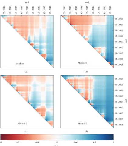
[image:15.600.91.513.69.551.2]G-1
Figure 17:Geometric mean return obtained within different periods of time.The geometric mean return computed between time “start” and “end” using the Sharpe ratio optimisation for the baseline (a), Method 1 (b), Method 2 (c), and Method 3 (d). Note that, for visualization purposes, the figure shows the translated geometric mean return G-1. Shades of red refer to negative returns and shades of blue to positive ones (see colour bar).
(Figure 17(b)), Method 2 (Figure 17(c)), and Method 3 (Figure 17(d)).
Data Availability
The data used to support the findings of this study are available from the corresponding author upon request.
Conflicts of Interest
The authors declare that they have no conflicts of interest.
References
[1] A. ElBahrawy, L. Alessandretti, A. Kandler, R. Pastor-Satorras, and A. Baronchelli, “Evolutionary dynamics of the cryptocur-rency market,” Royal Society Open Science, vol. 4, no. 11, November, 170623, 9 pages, 2017.
[2] G. Hileman and M. Rauchs, “Global Cryptocurrency Bench-marking Study,”Cambridge Centre for Alternative Finance, 2017. [3] Binance.com. (2017) Binance https://www.binance.com/. [4] Dunamu. (2017) Upbit https://upbit.com/.
[6] S. Foley, J. R. Karlsen, and T. J. Putniii, “Sex, Drugs, and Bitcoin: How Much Illegal Activity Is Financed Through Cryptocurren-cies?”SSRN Electronic Journal.
[7] S. Nakamoto,Bitcoin: A peer-to-peer electronic cash system, A peer-to-peer electronic cash system, Bitcoin, 2008.
[8] J. Barrdear and M. Kumhof, “The Macroeconomics of Central Bank Issued Digital Currencies,”SSRN Electronic Journal. [9] The Dash Network, (2018) Dash https://www.dash.org. [10] Ethereum Foundation (Stiftung Ethereum). (2018) Ethereum.
https://www.ethereum.org/.
[11] Ripple. (2013) Ripple https://ripple.com/. [12] (2018) Iota https://iota.org/.
[13] A. Baronchelli, “The emergence of consensus: a primer,”Royal
Society Open Science, vol. 5, no. 2, February, 172189, 13 pages,
2018.
[14] G. P. Dwyer, “The economics of Bitcoin and similar private digital currencies,”Journal of Financial Stability, vol. 17, pp. 81– 91, 2015.
[15] R. B¨ohme, N. Christin, B. Edelman, and T. Moore, “Bitcoin: Economics, technology, and governance,”Journal of Economic
Perspectives (JEP), vol. 29, no. 2, pp. 213–238, 2015.
[16] M. J. Casey and P. Vigna, “Bitcoin and the digital-currency revolution,”The Wall Street Journal, vol. 23, 2015.
[17] S. Trimborn and W. K. H¨ardle, “Crix or Evaluating Blockchain Based Currencies,”SSRN Electronic Journal, 2016.
[18] M. Iwamura, Y. Kitamura, and T. Matsumoto, “Is bitcoin the only cryptocurrency in the town? economics of cryptocurrency and friedrich a. hayek,”SSRN Electronic Journal, 2014.
[19] M. A. Cusumano, “The Bitcoin ecosystem,”Communications of
the ACM, vol. 57, no. 10, pp. 22–24, 2014.
[20] K. Wu, S. Wheatley, and D. Sornette,Classification of crypto-coins and tokens from the dynamics of their power law
capital-isation distributions , arXiv preprint, 1803.03088, 2018.
[21] A. Lamarche-Perrin, A. Orl´ean, and P. Jensen, “Coexistence of several currencies in presence of increasing returns to adoption,”Physica A: Statistical Mechanics and its Applications, vol. 496, pp. 612–619, 2018.
[22] P. M. Krafft, N. Della Penna, and A. S. Pentland, “An Experimen-tal Study of Cryptocurrency Market Dynamics,” inProceedings
of the the 2018 CHI Conference, pp. 1–13, Montreal QC, Canada,
April 2018.
[23] A. Rogojanu, L. Badea et al., “The issue of competing currencies. case studybitcoin,”Theoretical and Applied Economics, vol. 21, no. 1, pp. 103–114, 2014.
[24] L. H. White, “The market for cryptocurrencies,” the Cato
Journal, vol. 35, no. 2, pp. 383–402, 2015.
[25] P. Ceruleo,Bitcoin: a rival to fiat money or a speculative financial
asset?, 2014.
[26] M. N. Sayed and N. A. Abbas, “Impact of crypto-currency on emerging market focus on gulf countries,”Life Science Journal, vol. 15, no. 1, 2018.
[27] M. A. Javarone and C. S. Wright, “From Bitcoin to Bitcoin Cash: a network analysis,” inProceedings of the the 1st Workshop, pp. 77–81, Munich, Germany, June 2018.
[28] Y. Sovbetov,Factors influencing cryptocurrency prices: Evidence
from bitcoin, ethereum, dash, litcoin, and monero, Factors
influencing cryptocurrency prices, Evidence from bitcoin, 2018. [29] F. Parino, M. G. Beir´o, and L. Gauvin, “Analysis of the Bitcoin blockchain: socio-economic factors behind the adoption,”EPJ
Data Science, vol. 7, no. 1, 2018.
[30] S. Beguˇsi´c, Z. Kostanjˇcar, H. Eugene Stanley, and B. Podobnik, “Scaling properties of extreme price fluctuations in Bitcoin markets,”Physica A: Statistical Mechanics and its Applications, vol. 510, pp. 400–406, 2018.
[31] P. Ciaian, M. Rajcaniova, and D. Kancs, “The economics of BitCoin price formation,”Applied Economics, vol. 48, no. 19, pp. 1799–1815, 2016.
[32] T. Guo and N. Antulov-Fantulin,Predicting short-term bitcoin
price fluctuations from buy and sell orders , arXiv preprint, 2018.
[33] G. Gajardo, W. D. Kristjanpoller, and M. Minutolo, “Does Bitcoin exhibit the same asymmetric multifractal cross-correlations with crude oil, gold and DJIA as the Euro, Great British Pound and Yen?”Chaos, Solitons & Fractals, vol. 109, pp. 195–205, 2018.
[34] N. Gandal and H. Halaburda, “Can we predict the winner in a market with network effects? Competition in cryptocurrency market,”Games, vol. 7, no. 3, p. 16, 2016.
[35] H. Elendner, S. Trimborn, B. Ong, T. M. Lee et al., The cross-section of crypto-currencies as financial assets: An overview, Humboldt University, Berlin, Germany, 2016.
[36] D. Enke and S. Thawornwong, “The use of data mining and neural networks for forecasting stock market returns,”Expert
Systems with Applications, vol. 29, no. 4, pp. 927–940, 2005.
[37] W. Huang, Y. Nakamori, and S.-Y. Wang, “Forecasting stock market movement direction with support vector machine,”
Computers & Operations Research, vol. 32, no. 10, pp. 2513–2522,
2005.
[38] P. Ou and H. Wang, “Prediction of Stock Market Index Move-ment by Ten Data Mining Techniques,”Modern Applied Science
(MAS), vol. 3, no. 12, 2009.
[39] M. Gavrilov, D. Anguelov, P. Indyk, and R. Motwani, “Mining the stock market: Which measure is best?” inProceedings of the Sixth ACM SIGKDD International Conference on Knowledge
Discovery and Data Mining (KDD-2001), pp. 487–496, USA,
August 2000.
[40] K. S. Kannan, P. S. Sekar, M. M. Sathik, and P. Arumugam, “Financial stock market forecast using data mining techniques,”
inProceedings of the International MultiConference of Engineers
and Computer Scientists 2010, IMECS 2010, pp. 555–559, Hong
Kong, March 2010.
[41] A. F. Sheta, S. E. M. Ahmed, and H. Faris, “A comparison between regression, artificial neural networks and support vector machines for predicting stock market index,”Soft
Com-puting, vol. 7, p. 8, 2015.
[42] P. Chang, C. Liu, C. Fan, J. Lin, and C. Lai, “An Ensemble of Neural Networks for Stock Trading Decision Making,” in
Emerging Intelligent Computing Technology and Applications.
With Aspects of Artificial Intelligence, vol. 5755 ofLecture Notes
in Computer Science, pp. 1–10, Springer Berlin Heidelberg,
Berlin, Heidelberg, 2009.
[43] I. Madan, S. Saluja, and A. Zhao, Automated bitcoin trading via machine learning algorithms, 2015.
[44] H. Jang and J. Lee, “An Empirical Study on Modeling and Prediction of Bitcoin Prices with Bayesian Neural Networks Based on Blockchain Information,” IEEE Access, vol. 6, pp. 5427–5437, 2017.
[45] S. McNally, J. Roche, and S. Caton, “Predicting the Price of Bitcoin Using Machine Learning,” inProceedings of the 2018 26th Euromicro International Conference on Parallel, Distributed
and Network-based Processing (PDP), pp. 339–343, Cambridge,
[46] K. Hegazy and S. Mumford, Comparitive automated bitcoin trading strategies. 2016.
[47] A. G. Shilling, “Market Timing: Better Than a Buy-and-Hold Strategy,”Financial Analysts Journal, vol. 48, no. 2, pp. 46–50, 1992.
[48] Z. Jiang and J. Liang, “Cryptocurrency portfolio management with deep reinforcement learning,” inProceedings of the 2017
Intelligent Systems Conference (IntelliSys), pp. 905–913, London,
September 2017.
[49] Traderobot package, https://github.com/owocki/pytrader. [50] Cryptobot package, https://github.com/AdeelMufti/CryptoBot.
[51] Cryptocurrencytrader package, https://github.com/llens/Cryp-toCurrencyTrader.
[52] Btctrading package https://github.com/bukosabino/btctrading. [53] Bitpredict package, https://github.com/cbyn/bitpredict. [54] Bitcoin bubble burst, https://bitcoinbubbleburst.github.io/. [55] J. H. Friedman, “Stochastic gradient boosting,”Computational
Statistics & Data Analysis, vol. 38, no. 4, pp. 367–378, 2002.
[56] S. Hochreiter and J. Schmidhuber, “Long short-term memory,”
Neural Computation, vol. 9, no. 8, pp. 1735–1780, 1997.
[57] W. Brock, J. Lakonishok, and B. LeBaron, “Simple technical trading rules and the stochastic properties of stock returns,”The
Journal of Finance, vol. 47, no. 5, pp. 1731–1764, 1992.
[58] T. Kilgallen, “Testing the simple moving average across com-modities, global stock indices, and currencies,” Journal of
Wealth Management, vol. 15, no. 1, pp. 82–100, 2012.
[59] B. LeBaron, “The stability of moving average technical trading rules on the dow jones index,” Tech. Rep., 2000.
[60] C. A. Ellis and S. A. Parbery, “Is smarter better? A comparison of adaptive, and simple moving average trading strategies,”
Research in International Business and Finance, vol. 19, no. 3, pp.
399–411, 2005.
[61] coinmarketcap.com, https://coinmarketcap.com/.
[62] G. T. Friedlob and F. J. Plewa Jr, “Understanding return on investment,” in1em plus 0.5em minus 0.4em, John Wiley Sons, 4em, 1996.
[63] T. Chen and C. Guestrin, “XGBoost: a scalable tree boosting system,” inProceedings of the 22nd ACM SIGKDD International Conference on Knowledge Discovery and Data Mining, KDD 2016, pp. 785–794, August 2016.
[64] Inc. (2018) Kaggle, https://www.kaggle.com/.
[65] Z. C. Lipton, J. Berkowitz, and C. Elkan,A critical review of
recurrent neural networks for sequence learning , arXiv preprint,
2015.
[66] Bitcoinwiki, “Comparison of exchanges,” Comparison of
ex-changes, 2017, https://en.bitcoin.it/wiki/Comparison of
ex-changes.
[67] H. S. Moat, C. Curme, A. Avakian, D. Y. Kenett, H. Eugene Stanley, and T. Preis, “Quantifying wikipedia usage patterns before stock market moves,”Scientific Reports, vol. 3, 2013. [68] D. Kondor, I. Csabai, J. Sz¨ule, M. P´osfai, and G. Vattay,
“Inferring the interplay between network structure and market effects in Bitcoin,”New Journal of Physics, vol. 16, no. 12, 2014. [69] L. Kristoufek, “What are the main drivers of the bitcoin price?
Evidence from wavelet coherence analysis,”PLoS ONE, vol. 10, no. 4, 2015.
[70] D. Garcia and F. Schweitzer, “Social signals and algorithmic trading of Bitcoin,”Royal Society Open Science, vol. 2, no. 9, 2015.
[71] L. Kristoufek, “BitCoin meets Google Trends and Wikipedia: Quantifying the relationship between phenomena of the Inter-net era,”Scientific Reports, vol. 3, 2013.
[72] A. Urquhart, “What causes the attention of Bitcoin?”Economics
Letters, vol. 166, pp. 40–44, 2018.
[73] D. Garcia, C. J. Tessone, P. Mavrodiev, and N. Perony, “The dig-ital traces of bubbles: Feedback cycles between socio-economic signals in the Bitcoin economy,”Journal of the Royal Society
Interface, vol. 11, no. 99, article no. 0623, 2014.
[74] S. Wang and J. Vergne, “Correction: Buzz Factor or Innovation Potential: What Explains Cryptocurrencies’ Returns?” PLoS ONE, vol. 12, no. 5, p. e0177659, 2017.
[75] T. R. Li, A. S. Chamrajnagar, X. R. Fong, N. R. Rizik, and F. Fu,
Sentiment-based prediction of alternative cryptocurrency price
fluctuations using gradient boosting tree model , arXiv preprint,
Hindawi
www.hindawi.com Volume 2018
Mathematics
Journal ofHindawi
www.hindawi.com Volume 2018
Mathematical Problems in Engineering Applied Mathematics Hindawi
www.hindawi.com Volume 2018
Probability and Statistics Hindawi
www.hindawi.com Volume 2018
Hindawi
www.hindawi.com Volume 2018
Mathematical PhysicsAdvances in
Complex Analysis
Journal ofHindawi
www.hindawi.com Volume 2018
Optimization
Journal ofHindawi
www.hindawi.com Volume 2018
Hindawi
www.hindawi.com Volume 2018 Engineering Mathematics
International Journal of
Hindawi
www.hindawi.com Volume 2018
Operations Research
Journal of
Hindawi
www.hindawi.com Volume 2018
Function Spaces
Abstract and Applied AnalysisHindawi
www.hindawi.com Volume 2018
International Journal of Mathematics and Mathematical Sciences
Hindawi
www.hindawi.com Volume 2018
Hindawi Publishing Corporation
http://www.hindawi.com Volume 2013 Hindawi
www.hindawi.com
World Journal
Volume 2018
Hindawi
www.hindawi.com Volume 2018Volume 2018
Numerical Analysis
Numerical Analysis
Numerical Analysis
Numerical Analysis
Numerical Analysis
Numerical Analysis
Numerical Analysis
Numerical Analysis
Numerical Analysis
Numerical Analysis
Numerical Analysis
Numerical Analysis
Advances inAdvances in Discrete Dynamics in Nature and Society Hindawiwww.hindawi.com Volume 2018
Hindawi www.hindawi.com
Differential Equations
International Journal of
Volume 2018 Hindawi
www.hindawi.com Volume 2018
Decision Sciences
Hindawi
www.hindawi.com Volume 2018
Analysis
International Journal of
Hindawi
www.hindawi.com Volume 2018