City, University of London Institutional Repository
Citation
:
Movahedi, Y., Cukier, M., Andongabo, A. and Gashi, I. (2017). Cluster-based
Vulnerability Assessment Applied to Operating Systems. In: 2017 13th European
Dependable Computing Conference (EDCC). (pp. 18-25). IEEE. ISBN 978-1-5386-0602-5
This is the accepted version of the paper.
This version of the publication may differ from the final published
version.
Permanent repository link:
http://openaccess.city.ac.uk/id/eprint/17585/
Link to published version
:
Copyright and reuse:
City Research Online aims to make research
outputs of City, University of London available to a wider audience.
Copyright and Moral Rights remain with the author(s) and/or copyright
holders. URLs from City Research Online may be freely distributed and
linked to.
City Research Online: http://openaccess.city.ac.uk/ [email protected]
Cluster-based Vulnerability Assessment
Applied to Operating Systems
Yazdan Movahedi and Michel Cukier
Center for Risk and Reliability University of Maryland
College Park, USA {ymovahed, mcukier}@umd.edu
Ambrose Andongabo and Ilir Gashi
Center for Software Reliability City University London
London, U.K.
{ambrose.andongabo.1, ilir.gashi.1}@city.ac.uk
Abstract— Organizations face the issue of how to best allocate their security resources. Thus, they need an accurate method for assessing how many new vulnerabilities will be reported for the operating systems (OSs) they use in a given time period. Our approach consists of clustering vulnerabilities by leveraging the text information within vulnerability records, and then simulating the mean value function of vulnerabilities by relaxing the monotonic intensity function assumption, which is prevalent among the studies that use software reliability models (SRMs) and nonhomogeneous Poisson process (NHPP) in modeling. We applied our approach to the vulnerabilities of four OSs: Windows, Mac, IOS, and Linux. For the OSs analyzed in terms of curve fitting and prediction capability, our results, compared to a power-law model without clustering issued from a family of SRMs, are more accurate in all cases we analyzed.
Keywords— Vulnerability assessment, Nonhomogeneous Poisson process, Clustering, Software reliability models
I. INTRODUCTION
Security decision makers often use public data sources1 to
help make better decisions on, for example, what security products to choose, check for security trends, and estimate when new vulnerabilities that affect their installations will be publically reported. Several studies have applied software reliability models (SRMs) to estimate times between public reports of vulnerabilities [1]–[6]. The studies we are aware of estimate all vulnerabilities together. We postulate that such analysis may miss some trends that apply to separate categories of vulnerabilities, rather than all vulnerabilities together. Moreover, SRMs assume vulnerability detection to be an independent process. However, this process might not be independent due, for example, to the discovery of a new type of vulnerability that might prompt attackers to look for similar vulnerabilities [7]. This assumption may lead to sub-optimal predictions on the next reporting date of vulnerability, or the total number of new vulnerabilities reported in the next time interval. One way to mitigate these issues is to split vulnerabilities into separate clusters and ensure that the clusters are independent.
1 https://nvd.nist.gov/, https://exploit-db.com/ http://www.cvedetails.com/
In this paper we present an approach that does the following: - uses existing clustering techniques to group vulnerabilities into distinct clusters, using the textual information reported in these vulnerabilities as a basis for constructing the clusters;
- uses existing SRMs to make predictions on the number of new vulnerabilities that will be discovered in a given time period in the future for each of those clusters for a given OS;
- superposes the SRMs used for each cluster together into a single model for predicting the number of new vulnerabilities that will be discovered in a given time period for a given OS.
We have applied our approach on vulnerabilities of four different OSs: Windows (Microsoft), Mac (Apple), IOS (Cisco) and Linux. For these OSs, our approach when compared to a power-law model without clustering issued from a family of SRMs, gives more accurate curve fittings and predictions in all cases we analyzed.
The rest of the paper is structured as follows. Section II presents the related work. Section III details the dataset and how we processed the data. Section IV details the analysis. Section V presents the obtained results. Section VI discusses the results and lists the limitations. Finally, Section VII concludes the paper.
II. RELATED WORK
Rescorla [2], [3] proposed a VDM to find the number of undiscovered vulnerabilities for some OSs. In [4]–[6], Alhazmi and Malaiya proposed some regression models to simulate the vulnerability disclosure rate and predict the number of vulnerabilities that may potentially be present but may not yet have been found. Some studies have tried to increase the accuracy of vulnerability modeling. Joh et al. [14] proposed a new approach for modeling the skewness in vulnerability datasets by modifying common S-shaped models like Weibull and Gamma. However, all these models assume that the software under study has a finite number of vulnerabilities to be discovered [8]. While, in reality, releasing new patches might be accompanied by introducing new vulnerabilities to the product and dynamically change the number of vulnerabilities for a product. All these models provide better curve fitting results than predictions. This is because a model may provide an excellent fit for the available data points, but if the future detection trends are not consistent with the model, the model doesn’t predict well [14].
In addition to the vulnerabilities publication dates, software source code has been used for vulnerability assessment in the context of VDMs. Kim et al. [15] introduced a VDM based on shared source code measurements among multi-version software systems. In [16], Ozment and Schechter employed a reliability growth model to analyze the security of the OpenBSD OS by examining its source code and the rate at which new code has been introduced. Source code also proved not to be an adequately efficient measure in terms of prediction [7].
Clustering is a method of structuring data according to similarities and dissimilarities into natural groupings [17]. Clustering for vulnerabilities can be used for splitting real-world exploited vulnerabilities from those which were exploited during software test (Proof-of-Concept Exploits) [18], detecting exploited vulnerabilities versus non-exploited ones when there is not enough information about some vulnerabilities in database [19]. Lee et al. [20] investigated a distributed denial of service (DDoS) attack detection method using cluster analysis. Shahzad et al. [21] conducted a descriptive statistical analysis of a large software vulnerability dataset employing clustering on type-based vulnerability data. Huang et al. [22] classified NVD vulnerabilities employing several clustering algorithms to create a relatively objective classification criterion among the vulnerabilities.
III. DATASET AND DATA PROCESSING
The data used in this paper has been collected from the National Vulnerability Database (NVD) maintained by NIST. We developed Python scripts to scrape the publicly available data on vulnerabilities from NVD. We then stored the data in our own database, and identified each vulnerability by its Common Vulnerability Enumeration (CVE) identifier. We used the CVE ID to compare the reporting date of each vulnerability in NVD, with the dates in other public repositories on vulnerabilities2. We then update the reporting date on our
database to the earliest date that a given vulnerability was known
2 We looked at the following ones:http://www.cvedetails.com/,
https://cxsecurity.com/, http://www.security-database.com/ and http://www.securityfocus.com/
in any of these databases.
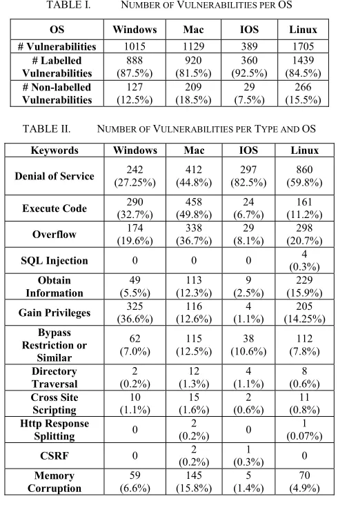
[image:3.612.318.563.313.684.2]For the rest of the paper, we will focus on the vulnerabilities reported for four well-known OSs: Windows(1995-2016), Mac (1997-2016), IOS (the OS associated with Cisco) (1992-2016), and Linux (1994-2016). We chose these OSs as they are most widely used, and had the most vulnerabilities in the databases. For each OS, we included all the vulnerabilities reported for any of its versions. For instance, all the vulnerabilities reported for mac_os, mac_os_server, mac_os_x, and mac_os_x_server were put together to create a vulnerability database for Mac. We did this to have enough data for each OS. The total number of vulnerabilities in NVD for these OSs is 4238. We used text information within vulnerabilities reports to then label the vulnerabilities. The keywords for labelling (e.g., denial, injection, buffer, execute) were extracted from these reports. Table I shows the total number of vulnerabilities as well as the number of labelled and non-labelled (vulnerabilities without any associated text information in the database) vulnerabilitiesfor these OSs. For the labelled vulnerabilities, we indicate the number and proportion of vulnerabilities associated with a specific keyword. Note that vulnerabilities can be labelled with more than one keyword. Details for each OS are in Table II.
TABLE I. NUMBER OF VULNERABILITIES PER OS
OS Windows Mac IOS Linux # Vulnerabilities 1015 1129 389 1705
# Labelled Vulnerabilities 888 (87.5%) 920 (81.5%) 360 (92.5%) 1439 (84.5%) # Non-labelled Vulnerabilities 127 (12.5%) 209 (18.5%) 29 (7.5%) 266 (15.5%)
TABLE II. NUMBER OF VULNERABILITIES PER TYPE AND OS
Keywords Windows Mac IOS Linux Denial of Service (27.25%) 242 (44.8%) 412 (82.5%) 297 (59.8%) 860
Execute Code (32.7%) 290 (49.8%) 458 (6.7%) 24 (11.2%) 161 Overflow (19.6%) 174 (36.7%) 338 (8.1%) 29 (20.7%) 298 SQL Injection 0 0 0 (0.3%) 4
Obtain Information 49 (5.5%) 113 (12.3%) 9 (2.5%) 229 (15.9%)
Gain Privileges (36.6%) 325 (12.6%) 116 (1.1%) 4 (14.25%) 205 Bypass
Restriction or Similar
62
(7.0%) (12.5%) 115 (10.6%) 38 (7.8%) 112
Directory Traversal 2 (0.2%) 12 (1.3%) 4 (1.1%) 8 (0.6%) Cross Site Scripting 10 (1.1%) 15 (1.6%) 2 (0.6%) 11 (0.8%) Http Response
Splitting 0
2
(0.2%) 0 (0.07%) 1
CSRF 0 (0.2%) 2 (0.3%) 1 0
For cluster analysis, we need to ensure that the features (keywords) are not correlated. Therefore, we checked the Pearson correlation coefficient for every two keywords per OS. When we found statistically significant correlation, we merged the correlated keywords with a title which included both terms. For instance, due to the high correlation of .99 (p-value<0.001, : = 0) between “Execute” and “Code” for all Oss, these terms were treated as “Execute Code”. The same applied for the keywords “SQL” and “Injection”. No other significant correlation was observed.
For clustering, we used the HPCLUS (High Performance Clustering) procedure in SAS 9.4 with the k-means and k-modes algorithms for clustering nominal input variables. This procedure uses the least square method in k-means to compute cluster centroids. Each iteration reduces the criterion (e.g., the least squared criterion for Euclidean distance) until convergence is achieved or the maximum iteration number is reached [23]. Additionally, we set our method to cluster the data based upon the associated principal component analysis (PCA) scores derived from the linear combinations of binary attributes for each OS. PCA reduces the number of features that might be correlated to independent linear combinations of them [17].
To estimate the best number of clusters the aligned box criterion (ABC) method was used. The cubic clustering criterion (CCC) is another common metric which is usually used in clustering applications to find the most suitable number of clusters [24]. Tibshirani et al. [25] proposed a gap statistics method which leverages Monte Carlo simulation for detecting the best number of clusters in a database. However, the ABC method improves the CCC and gap statistics methods by leveraging a high-performance machine-learning based analysis structure [23]. In addition, within-cluster dispersion was also used as an error measure (also called a ‘Gap’) by the ABC method [25]. In order to find the best number of clusters, we applied the ABC method that compares the calculated Gap values over a range of possible k values. The best number of clusters occurs at the maximum peak value in Gap (k) [23]. We obtained 6, 6, 7, 7 clusters for Windows, Mac, IOS, and Linux, respectively.
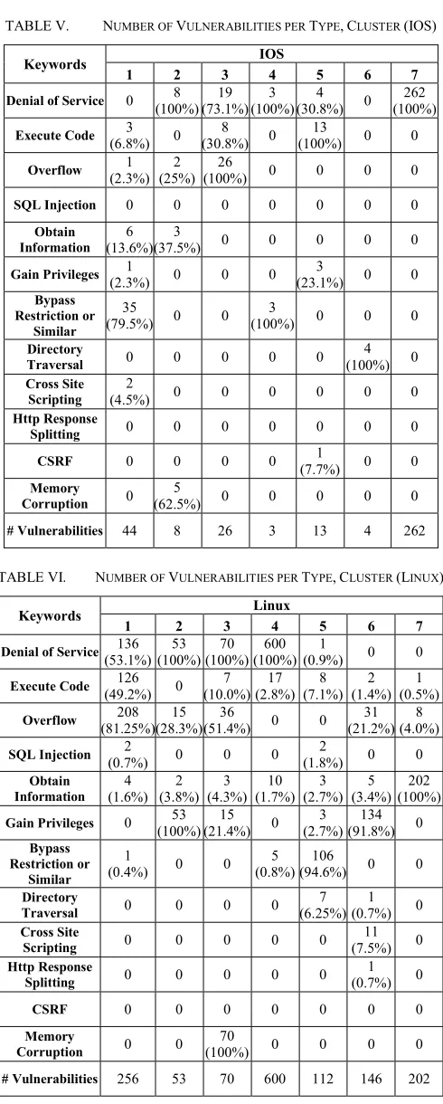
Tables III - VI lists the keywords associated with each of the six / seven clusters for Windows, Mac, IOS, and Linux respectively.
The most frequent keywords were selected to name the clusters with respect to the keywords’ weights information provided in Tables III - VI. We assumed that the keywords which covered at least 60% of vulnerabilities in each cluster can be good representatives of relative clusters.
Since, none of the keywords reach the weight threshold of 0.6 in the third cluster associated with Mac, the keyword with greatest weight (Denial of Service) was selected as the cluster’s label. All the OSs have one cluster with a similar name. There are also similarly named clusters within some OSs. However, analyzing their linear correlation, we did not find any significant relationship based on the Pearson correlation test. Table VII shows the cluster summaries for the OSs.
TABLE III. NUMBER OF VULNERABILITIES PER TYPE,CLUSTER
(WINDOWS)
Keywords Windows
1 2 3 4 5 6
Denial of Service (15.5%)16 (91.7%) 22 (33.3%) 6 (69.1%)188 (1.7%)5 (2.9%) 5
Execute Code (95.1%)98 (20.8%) 5 (83.3%) 15 0 0 (100%)171
Overflow (100%)103 (87.5%) 21 0 (6.25%)17 (11.0%)33 0
SQL Injection 0 0 0 0 0 0
Obtain Information
1 (1.0%) 0
1 (5.55%) 43 (15.8%) 4 (1.33%) 0
Gain Privileges (1.9%) 2 (58.3%) 14 0 0 (100%)300 (5.3%) 9
Bypass Restriction or
Similar 0 0 0
56 (20.6%) 5 (1.7%) 1 (0.6%) Directory
Traversal 0 0 0
1 (0.4%)
1 (0.3%) 0
Cross Site
Scripting 0 0 0
8 (2.9%) 0
2 (1.2%)
Http Response
Splitting 0 0 0 0 0 0
CSRF 0 0 0 0 0 0
Memory Corruption 9 (8.7%) 23 (95.8%) 18 (100%) 0
9 (3.0%) 0
# Vulnerabilities 103 24 18 272 300 171
TABLE IV. NUMBER OF VULNERABILITIES PER TYPE,CLUSTER (MAC)
Keywords Mac
1 2 3 4 5 6
Denial of Service (64.2%)174 0 (39.0%) 120 0 0 (100%)118
Execute Code (93.4%)253 0 0 (2.6%)3 (96.8%)90 (94.9%)112
Overflow (37.3%)101 0 23
(7.5%) 3 (2.6%) 93 (100%) 118 (100%)
SQL Injection 0 0 0 0 0 0
Obtain Information 1 (0.4%) 1 (6.7%) 103 (33.4%) 8
(7.0%) 0 0
Gain Privileges (4.4%)12 0 (32.1%) 99 (3.5%)4 0 (0.8%)1
Bypass Restriction or
Similar
0 0 0 (100%)115 0 0
Directory Traversal 3 (1.1%) 0 8 (2.6%) 1
(0.9%) 0 0
Cross Site
Scripting 0
15
(100%) 0 0 0 0
Http Response
Splitting 0
2
(13.3%) 0 0 0 0
CSRF 0 0 (0.3%) 1 (0.9%)1 0 0
Memory
Corruption (51.3%)139 0 (1.6%) 5 (0.9%)1 0 0
TABLE V. NUMBER OF VULNERABILITIES PER TYPE,CLUSTER (IOS)
Keywords IOS
1 2 3 4 5 6 7
Denial of Service 0 (100%) 8 (73.1%)19 (100%) 3 (30.8%)4 0 (100%)262
Execute Code (6.8%) 3 0 (30.8%)8 0 (100%) 13 0 0
Overflow (2.3%) 1 (25%) 2 (100%) 26 0 0 0 0
SQL Injection 0 0 0 0 0 0 0
Obtain Information
6 (13.6%)
3
(37.5%) 0 0 0 0 0
Gain Privileges (2.3%) 1 0 0 0 (23.1%)3 0 0
Bypass Restriction or
Similar
35
(79.5%) 0 0
3
(100%) 0 0 0
Directory
Traversal 0 0 0 0 0
4 (100%) 0
Cross Site Scripting
2
(4.5%) 0 0 0 0 0 0
Http Response
Splitting 0 0 0 0 0 0 0
CSRF 0 0 0 0 (7.7%) 1 0 0
Memory
Corruption 0
5
(62.5%) 0 0 0 0 0
# Vulnerabilities 44 8 26 3 13 4 262
TABLE VI. NUMBER OF VULNERABILITIES PER TYPE,CLUSTER (LINUX)
Keywords Linux
1 2 3 4 5 6 7
Denial of Service (53.1%) 136 (100%) 53 (100%) 70 (100%) 600 (0.9%) 1 0 0
Execute Code (49.2%) 126 0 (10.0%)7 (2.8%) 17 (7.1%) 8 (1.4%)2 (0.5%)1
Overflow (81.25%)208 (28.3%)15 (51.4%)36 0 0 (21.2%)31 (4.0%)8
SQL Injection (0.7%) 2 0 0 0 (1.8%) 2 0 0
Obtain Information
4 (1.6%)
2 (3.8%)
3 (4.3%)
10 (1.7%)
3 (2.7%)
5 (3.4%)
202 (100%)
Gain Privileges 0 (100%) 53 (21.4%)15 0 (2.7%) 3 (91.8%)134 0
Bypass Restriction or
Similar
1
(0.4%) 0 0
5 (0.8%)
106
(94.6%) 0 0
Directory
Traversal 0 0 0 0
7 (6.25%)
1 (0.7%) 0
Cross Site
Scripting 0 0 0 0 0
11 (7.5%) 0
Http Response
Splitting 0 0 0 0 0
1 (0.7%) 0
CSRF 0 0 0 0 0 0 0
Memory
Corruption 0 0 (100%) 70 0 0 0 0
# Vulnerabilities 256 53 70 600 112 146 202
TABLE VII. CLUSTER COMPOSITION
OS number Cluster Prevalent Keywords Cluster Name
Windo
w
s
1 Execute code, Overflow EO
2 DoS , Overflow, Memory corruption DOM
3 Execute code, Memory corruption EM
4 DoS D
5 Gain privileges G
6 Execute code E
Ma
c
1 DoS, Execute code DE
2 Cross site scripting C
3 DoS D
4 Bypass a restriction B
5 Execute code, Overflow EO
6 Dos, Execute code, Overflow DEO
IOS
1 Bypass a restriction B
2 DoS, Memory corruption DM
3 DoS , Overflow DO
4 DoS, Bypass a restriction DB
5 Execute code E
6 Directory Traversal DT
7 DoS D
Lin
ux
1 DoS , Overflow DO
2 Dos, Gain privileges DG
3 DoS, Memory corruption DM
4 DoS D
5 Bypass a restriction B
6 Gain privileges G
7 Obtain Information O IV.ANALYSIS
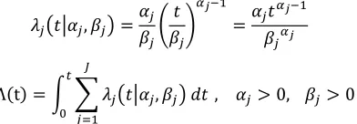
A nonhomogeneous Poisson process (NHPP) is often used when modeling the mean cumulative number of failures (MCF) ( ) for repairable systems and for software reliability evaluations. The core assumption is that the number of detected failures follows a nonhomogeneous Poisson process. In the case of NHPP-based repairable systems, the intensity function
λ( )= [ ( )]/ is often assumed to be a monotonic function of t. Similarly, in NHPP-based software reliability models (SRMs), the intensity function (the detection rate of software errors) is considered to be a monotonic function [26].
Let us expand the discussion for a software when there exists more than one type of error. When any type of error independently causes the software normal function to be compromised, then the superposition model represents the software failures. Let us assume that we are dealing with vulnerabilities classified into independent clusters. Let ( ) denote the NHPP for the vulnerabilities from the cluster in (0 t], with intensity function ( | , ) where the function form of ( | , ) is given and the values of the parameters ,
from any cluster ( ), = 1,2, … is independent. A process ( ) = ∑ ( ), which counts the total number of vulnerabilities in the interval (0 t] for the superposition model, is also a non-homogeneous Poisson process with an intensity function ( | , ) = ( | , ) + ⋯ + ( | , ), where
= { , … , } , = { , … , }. Since the superposition
model remains an NHPP (all intensity functions are NHPPs), the associated superposition model can be applicable [26]. The most prevalent types of intensity functions for NHPPs are power-law and log-linear (exponential) models. We used the power-law model since this model provided better curve fitting results compared to the log-linear model. In such case, the equations become:
, = =
Λ(t) = , , > 0, > 0
In this paper, we expect to obtain better assessment results when relaxing the monotonicity assumption of the intensity function that is prevalent in SRMs and VDMs. We created independent clusters that can be modeled using separate NHPPs. Selecting a power-law intensity function, we considered two models for this paper. The first model is a NHPP-based SRM, which uses clustered data (including all the labeled and non-labeled vulnerabilities). The second model is the superposition of the NHPPs fitted to the clustered data (only the labelled vulnerabilities can be used to create the clusters), which relaxes the monotonicity assumption of the intensity function. The purpose of both models is to fit and predict the total number of reported vulnerabilities (labeled and non-labeled) over the study period.
The analysis was done in two steps. First, we used the time difference between vulnerability report dates to find the model parameters from the process of fitting NHPPs to the data (clustered and non-clustered). Non-homogeneity of the clusters were also validated in this step by looking at Laplace-trend test results provided by MiniTab 16 to see whether there were meaningful trends in clusters. Second, we used the estimated parameters and the models, and simulated corresponding MCFs (one MCF for clustered data, and one for non-clustered data) starting from =0 and time intervals of 10 days.
V. RESULTS
[image:6.612.75.271.212.280.2]In this section we will provide the results regarding estimation (comparing the results between clustered data and non-clustered data) and forecasting (comparing the obtained predictions with clustered data and non-clustered data using a subset of the data).
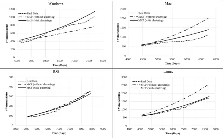
Figure 1 shows the observed vulnerability data, the MCF obtained without clustering the data and the superimposed MCF when clustering is applied for all the OSs in our study. For Windows, the MCF with clustering is more conservative during roughly the first 3000 days then the MCF without clustering becomes more conservative. The real data crosses the estimates between roughly 2000 and 3000 days. Besides this period, the
MCF with and without clustering provide more conservative estimates. For IOS, the MCF with and without clustering as well as the real data are almost overlapping. For Mac and Linux, the MCF with clustering is above the MCF without clustering, providing a more conservative estimation. The real data is above the MCF without clustering and for a short period above the MCF with clustering. Thus for Mac and Linux, the MCF with clustering provide more conservative and accurate estimates.
The analysis of forecasting is done for the final third of the time period from the beginning of the vulnerability discovery process. During the training period (first two thirds of the time period), all the available data are used to estimate model parameters. Figure 2 shows the forecast of the number of vulnerabilities based on the MCFs calculated with and without clustering compared to the observed vulnerabilities. For the vulnerabilities associated with Windows, the forecast with clustering leads to more conservative and more accurate estimates compared to non-clustering. In addition, the forecast without clustering remains below the observed vulnerability data (real data) for the prediction time period which started after day 5088. Both models lead to more conservative predictions for the vulnerabilities associated with Mac. However, the clustering-based MCF trajectory provides more accurate predictions. For IOS the forecast without clustering is more conservative compared to the forecast with clustering. When the MCF without clustering remains above the real data (which is good), it is not the case of the forecast with clustering where the real data crosses the forecast after Day 7500. For Linux, the predictions with clustering and the real observed data are close but the forecast remains above the real data and thus provides conservative estimation (which is good). The clustering-based MCF is, however, much more accurate than that of the non-clustering MCF.
We applied the Chi-square (χ ) goodness of fit test [14] to see how well each model fits the datasets for both estimation and forecasting. The Chi-square statistic is calculated using the following equation:
χ = ( − )
Where and are the simulated and real observed values at time point, respectively. N is the number of observations (the time blocks used for simulation). For the fit to be acceptable, the corresponding χ critical value should be greater than the χ statistic value for the given alpha level and degrees of freedom. We selected an alpha level of 0.05. The null hypothesis indicates that the actual distribution is well described by the fitted model. Hence, if the P-value of the χ test is below 0.05, then the fit will be considered to be unsatisfactory. A p-value closer to 1 indicates a better fit.
Windows Mac
[image:7.612.85.530.55.327.2]IOS Linux
Fig. 1. Comparison of Clustered and Non-clustered MCFs with Vulnerability Data
Windows Mac
IOS Linux
[image:7.612.85.530.372.646.2]The normalized root mean square error (NRMSE) is often used. However, Mentaschi et al. [28] showed that for some applications (e.g., high fluctuation of real data) the higher values of NRMSE are not always a reliable indicator of the accuracy of simulations. To remedy the situation, a corrected estimator HH was proposed by Hanna and Heinold [29]:
= ∑ ( − )
∑
where is the simulated data, is the observation and N is the number of observations (the time blocks used for simulation). The closer to zero HH is, the more accurate the model.
Table VIII contains the Chi-square goodness of fit test for the clustering-based MCF and the MCF without clustering, the values of R , and HH for the vulnerabilities of the four OSs in our study.
We considered the entire dataset for analyzing estimation accuracy. When considering the entire dataset, both estimations (with/without clustering) are statistically sound for all OSs but one (Mac, without clustering) with P-values greater than 0.05. The Chi-square test results indicate that both fits are reasonably good in most cases except the case associated with the non-clustered based MCF on Mac data. The R statistics show that estimations based on clustering are more accurate than the ones without clustering. HH results also show that clustering based estimations came up with smaller errors compared with non-clustering. For all OSs in our study the estimations based on clustering were more accurate in all cases. In addition, the MCF model without clustering was not statistically adequate to model the vulnerability data in one case (Mac).
Table IX contains the Chi-square goodness of fit test for prediction values of the clustering and non-clustering-based MCF, the R and HH prediction values for the vulnerabilities of the four OSs in our study. We considered the common 66% splits between training and forecasting which means all the available data in the first two thirds of the study time period were used to estimate model parameters.
For the vulnerabilities associated with Windows, Mac, and Linux, all considered training/forecasting results using non-clustered data lead to statistically inadequate fits since all the relative P-values are zeros. For vulnerabilities associated with IOS, while both models came up with adequate fits based upon the Chi-squared test result, the clustering-based forecast is more accurate due to higher R-squared and lower HH values. For the other OSs, the predictions associated with clustered data are statistically sound with P-values greater than 0.05 and reasonably good R-squared and HH values. Thus, the forecasts based on clustering were more accurate in all cases. In addition, the MCF model without clustering was not statistically adequate to model the vulnerability data in three cases.
TABLE VIII. ESTIMATION ACCURACY FOR FOUR OSS
Estimation With clustering Without clustering
p-value R-sq HH p-value R-sq HH
Windows 1 0.975 0.098 1 0.945 0.145
Mac 0.052 0.851 0.242 0.028 0.837 0.326
IOS 1 0.987 0.084 1 0.972 0.098
Linux 1 0.995 0.06 1 0.992 0.099
TABLE IX. FORECASTING ACCURACY FOR FOUR OSS
Forecasting With clustering Without clustering
p-value R-sq HH p-value R-sq HH
Windows 0.792 0.838 0.104 0 0.558 0.196
Mac 0.115 0.577 0.238 0 -0.316 0.514
IOS 0.992 0.902 0.122 0.977 0.896 0.135
Linux 0.708 0.833 0.102 0 -1.822 0.367
VI. LIMITATIONS
The main limitation of the work we present in the paper is with regard to using SRMs as VDMs. Software reliability models usually assume that the time between failures represents total usage time of that product. What we are using is calendar time, which may not be a good proxy for usage. Crucially the difference in security is the difficulty in estimating the “attacker effort” - the total amount of time that an attacker spends in finding a vulnerability - which is something that is not needed for reliability (we assume the users accidentally encounter faults that lead to failures, hence usage time is a good enough proxy for time between failures). A useful discussion of this is given in [30]. Note that this limitation is not only for our work, but applies to research that uses SRMs as VDM and utilizes vulnerability data. However, attacker effort is something that is very difficult to estimate and quantify. The purpose of our research is hence to make as good a use as possible of the publically available security data to help with decision making. But at the same time to be clear about the limitations on what we can conclude from this analysis. The best we can say from the analysis we present is “the total number of vulnerabilities that will be reported in the NVD over an interval t for product x is y with confidence z”. And we show that we can do this prediction better with clustering than without clustering for four of the largest and most commonly used operating system families. For some decision makers this may be a valuable piece of additional information, which they can use in conjunction with data they have from their own installations, when deciding on security operating system/product choices, and provisioning of security support services to deal with new vulnerabilities.
VII.CONCLUSIONS
We presented an approach that: first, uses existing clustering techniques to group vulnerabilities into distinct clusters; second, uses an existing Non-Homogenous Poisson Process (NHPP) Software Reliability Model (SRM) to make predictions on the number of new vulnerabilities that will be discovered in a given time period for each of those clusters for a given OS; and finally, superimpose the SRMs used for each cluster together into a single model for predicting the number of new vulnerabilities that will be discovered in a given time period for a given OS.
We provided results from applying our approach to vulnerabilities of four different OSs: Windows, Mac, IOS, and Linux, and comparisons of the predictive accuracy of our approach compared with an NHPP model (with monotonic intensity function) that does not use clustering. We found that our approach with clustering, compared with the same modeling mechanism without clustering:
• Is statistically adequate in terms of model fitting and forecasting based upon the Chi-squared goodness of fit test results for all cases we analyzed, while the model without clustering was not statistically sound in 4 out of 8 cases analyzed.
• Gives more conservative forecasting results in all cases while the model without clustering was not conservative for Windows.
• Gives more accurate results for all the cases analyzed compared to non-clustering.
These results look encouraging, especially as they have been applied for some of the most widely used software products (operating systems) which tend to have the most number of vulnerabilities reported. In current and future work we will apply this approach to other widely used products such as web browsers and database systems.
ACKNOWLEDGMENT
This research is supported by NSF award #1223634, and the UK EPSRC project D3S (Diversity and defence in depth for security: a probabilistic approach).
REFERENCES
[1] M. R. Lyu, Ed., Handbook of software reliability engineering. Los Alamitos, Calif. : New York: IEEE Computer Society Press ; McGraw Hill, 1996.
[2] E. Rescorla, “Security holes... Who cares?,” presented at the USENIX Security, 2003.
[3] E. Rescorla, “Is finding security holes a good idea?,” IEEE Secur. Priv. Mag., vol. 3, no. 1, pp. 14–19, Jan. 2005.
[4] O. H. Alhazmi and Y. K. Malaiya, “Quantitative vulnerability assessment of systems software,” 2005, pp. 615–620.
[5] S. Woo, O. Alhazmi, and Y. Malaiya, “Assessing Vulnerabilities in Apache and IIS HTTP Servers,” 2006, pp. 103–110.
[6] O. H. Alhazmi and Y. K. Malaiya, “Application of Vulnerability Discovery Models to Major Operating Systems,” IEEE Trans. Reliab., vol. 57, no. 1, pp. 14–22, Mar. 2008.
[7] J. A. Ozment, “Vulnerability discovery & software security,” University of Cambridge, 2007.
[8] H. Okamura, M. Tokuzane, and T. Dohi, “Optimal Security Patch Release Timing under Non-homogeneous Vulnerability-Discovery Processes,” 2009, pp. 120–128.
[9] P. E. Verissimo et al., “Intrusion-tolerant middleware: the road to automatic security,” IEEE Secur. Priv. Mag., vol. 4, no. 4, pp. 54–62, Jul. 2006.
[10] H. Okamura, M. Tokuzane, and T. Dohi, “Quantitative Security Evaluation for Software System from Vulnerability Database,” J. Softw. Eng. Appl., vol. 06, no. 04, p. 15, Apr. 2013.
[11] W. A. Arbaugh, W. L. Fithen, and J. McHugh, “Windows of vulnerability: a case study analysis,” Computer, vol. 33, no. 12, pp. 52– 59, Dec. 2000.
[12] S. Frei, M. May, U. Fiedler, and B. Plattner, “Large-scale Vulnerability Analysis,” in Proceedings of the 2006 SIGCOMM Workshop on Large-scale Attack Defense, New York, NY, USA, 2006, pp. 131–138. [13] S. Frei, D. Schatzmann, B. Plattner, and B. Trammell, “Modeling the
Security Ecosystem - The Dynamics of (In)Security,” in Economics of Information Security and Privacy, Springer, Boston, MA, 2010, pp. 79– 106.
[14] H. Joh and Y. K. Malaiya, “Modeling Skewness in Vulnerability Discovery: Modeling Skewness in Vulnerability Discovery,” Qual. Reliab. Eng. Int., vol. 30, no. 8, pp. 1445–1459, Dec. 2014. [15] J. Kim, Y. K. Malaiya, and I. Ray, “Vulnerability Discovery in
Multi-Version Software Systems,” in 10th IEEE High Assurance Systems Engineering Symposium, 2007. HASE ’07, 2007, pp. 141–148. [16] A. Ozment and S. E. Schechter, “Milk or wine: does software security
improve with age?,” presented at the 15th USENIX Security Symposium, 2006.
[17] R. A. Johnson and D. W. Wichern, Applied multivariate statistical analysis, 6th ed. Upper Saddle River, N.J: Pearson Prentice Hall, 2007. [18] C. Sabottke, S. Octavian, and T. Dumitras, “Vulnerability Disclosure in the Age of Social Media: Exploiting Twitter for Predicting Real-World Exploits,” presented at the USENIX Security, 2015, vol. 15.
[19] A. Younis, Y. K. Malaiya, and I. Ray, “Assessing vulnerability exploitability risk using software properties,” Softw. Qual. J., vol. 24, no. 1, pp. 159–202, Mar. 2016.
[20] K. Lee, J. Kim, K. H. Kwon, Y. Han, and S. Kim, “DDoS attack detection method using cluster analysis,” Expert Syst. Appl., vol. 34, no. 3, pp. 1659–1665, Apr. 2008.
[21] M. Shahzad, M. Z. Shafiq, and A. X. Liu, “A Large Scale Exploratory Analysis of Software Vulnerability Life Cycles,” in Proceedings of the 34th International Conference on Software Engineering, Piscataway, NJ, USA, 2012, pp. 771–781.
[22] S. Huang, H. Tang, M. Zhang, and J. Tian, “Text Clustering on National Vulnerability Database,” in 2010 Second International Conference on Computer Engineering and Applications, 2010, vol. 2, pp. 295–299. [23] SAS® Enterprise MinerTM 14.2: High-Performance Procedures. Cary,
NC: SAS Institute Inc., 2016.
[24] W. S. Sarle, “Cubic Clustering Criterion,” SAS Institution Inc., Cary, NC, SAS® Technical Report A-108, 1983.
[25] R. Tibshirani, G. Walther, and T. Hastie, “Estimating the number of clusters in a data set via the gap statistic,” J. R. Stat. Soc. Ser. B Stat. Methodol., vol. 63, no. 2, pp. 411–423, Jan. 2001.
[26] T. Y. Yang and L. Kuo, “Bayesian computation for the superposition of nonhomogeneous poisson processes,” Can. J. Stat., vol. 27, no. 3, pp. 547–556, Sep. 1999.
[27] D. N. Gujarati and D. C. Porter, Basic Econometrics. McGraw-Hill Irwin, 2009.
[28] L. Mentaschi, G. Besio, F. Cassola, and A. Mazzino, “Problems in RMSE-based wave model validations,” Ocean Model., vol. 72, pp. 53– 58, Dec. 2013.
[29] S. R. Hanna, D. W. Heinold, A. P. I. H. and E. A. Dept, and E. R. & T. Inc, Development and application of a simple method for evaluating air quality models. American Petroleum Institute, 1985.