Conditional Regressive Random Forest Stereo-based Hand Depth Recovery

City, University of London Institutional Repository

Citation

:

Basaru, R. R., Child, C. H. T., Alonso, E. and Slabaugh, G. G. (2018).

Conditional Regressive Random Forest Stereo-based Hand Depth Recovery. 2017 IEEE

International Conference on Computer Vision Workshops (ICCVW), pp. 614-622. doi:

10.1109/ICCVW.2017.78

This is the accepted version of the paper.

This version of the publication may differ from the final published

version.

Permanent repository link:

http://openaccess.city.ac.uk/18088/

Link to published version

:

http://dx.doi.org/10.1109/ICCVW.2017.78

Copyright and reuse:

City Research Online aims to make research

outputs of City, University of London available to a wider audience.

Copyright and Moral Rights remain with the author(s) and/or copyright

holders. URLs from City Research Online may be freely distributed and

linked to.

City Research Online:

http://openaccess.city.ac.uk/

[email protected]

Abstract

This paper introduces Conditional Regressive Random Forest (CRRF), a novel method that combines a closed-form Conditional Random Field (CRF), using learned weights, and a Regressive Random Forest (RRF) that employs adaptively selected expert trees. CRRF is used to estimate a depth image of hand given stereo RGB inputs. CRRF uses a novel superpixel-based regression framework that takes advantage of the smoothness of the hand’s depth surface. A RRF unary term adaptively selects different stereo-matching measures as it implicitly determines matching pixels in a coarse-to-fine manner. CRRF also includes a pair-wise term that encourages smoothness between similar adjacent superpixels. Experimental results show that CRRF can produce high quality depth maps, even using an inexpensive RGB stereo camera and produces state-of-the-art results for hand depth estimation.

1.Introduction

Recently there has been surging interest in virtual and augmented reality devices [2, 4] that has in turn prompted research into natural approaches for interacting with such systems, e.g. hand gesture. While human body pose estimation from RGBD data may be considered a solved problem, open challenges remain for estimating hand pose as hands exhibit a high degree of self-occlusion and greater variation in orientation relative to the camera [22, 23]. We argue that the key to natural gestural interaction with next generation devices is robust hand pose estimation. An important design criterion for a hand pose estimation approach is the type of imaging sensor employed. RGBD sensors are a popular choice, as depth-based input provides good shape information, robustness to clutter and changes in ambient conditions. Using the depth channel, inference algorithms can be developed to estimate the hand pose [22, 23]. Despite the successes of such approaches, depth channel data capture poses several limitations, including poor form factor in egocentric applications, large energy consumption, poor near distance coverage, and inferior performance outdoors. Therefore, in this paper we focus instead on RGB data capture. By acknowledging that a single RGB camera does not provide enough shape and

structure information, we focus on a stereovision technique using two cameras.

The goal of our research is to extract robust hand depth information from stereo RGB inputs as a precursor to hand pose estimation. Depth estimation from two views has a long and rich history in computer vision, and fundamentally relates to establishing correct correspondences between images. However, the recovery of hand depth provides unique challenges that differentiates the problem from depth recovery of arbitrary scenes as expressed in [9]. Unlike generic scene depth estimation, there is significantly less texture in hand depth estimation, which makes stereo matching substantially more challenging. There is also high tendency of self-occlusion which manifests in changes in depth that might not reflect in a change in texture. For example, the occlusion of a finger on the palm will yield a change in depth but the color and the texture of the region of occlusion might remain largely unchanged as the color of the skin might be consistent (whether on the finger or on the palm region). This necessitates a new hand-specific depth estimation technique to outperform generic stereo matching algorithms.

Whilst recovery of hand depth provides unique challenges, the fact that the depth recovery task will only apply to a class of object (hand) means that stereo matching constraints can be learnt using a machine learning approach and tested on similar surfaces. This is particularly useful as we can better establish the matching criteria that can achieve the best stereo matches and hence disparity since we know the typical structure of the “scene” for which we are going to be estimating depth. In this work, we do not implement gesture recognition, instead we solely focus on recovering accurate depth. The proposed technique also relies on a robust hand segmentation procedure. We do not address hand segmentation in this paper as there is a large body of literature on this subject (see, for example, [7, 8]).

This paper proposes a novel, data-driven Conditional Regressive Random Forest (CRRF) framework. CRRF learns the mapping between a stereo image pair and high quality ground truth depth measurement. In so doing, we present an innovative combination of Regressive Random Forest and Conditional Random Fields to model this mapping. A major contribution of this research is the use of a machine learning framework to combine various stereo

Conditional Regressive Random Forest Stereo-based Hand Depth Recovery

Rilwan Remilekun Basaru

City, University of London

London, United Kingdom

Chris Child, Eduardo Alonso, Greg Slabaugh

City, University of London

matching criteria (multiple cost functions and window sizes) with the aim of implicitly determining stereo correspondences. Unlike conventional CRF methods that require iterative solutions, we derive a closed form solution to CRRF inference. We note our CRRF framework has much wider application, particularly to problems that can be posed using graph theory.

2.Related Work

The computer vision literature includes numerous methods of depth estimation, but for conciseness we focus on the most related approaches. Stereovision is based on the physical concept of stereopsis. This specifies that given the view of a scene from two perspectives, the shift undergone by corresponding pixels in both images varies such that it is inversely proportional to the distance from the camera. Hence the problem of depth recovery given a pair of images is reduced to establishing correct correspondences between both images. The Middlebury website [6] contains a large collection of stereo match algorithms and cost functions, as well as a test-bed for relative comparison.

Depth recovery from a single image is proposed in [18-20], modelling the depth estimation as a Markov Random Field (MRF) learning problem. The success of Deep Learning in computer vision has prompted recent approaches to model the problem with Convolutional Neural Networks (CNNs) [21]. While showing much promise, work to date has lacked stronger geometric features (like stereoscopic information) highly correlated

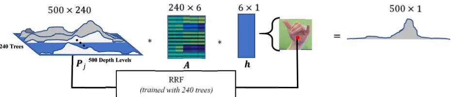
with depth. A closely related technique to ours is [5], where a data-driven approach has been taken to develop a near-infrared based depth camera. In this study, a two-layered Random Forest framework was used to establish the mapping between near infrared images of a scene consisting of articulated hand poses captured from modified RGB cameras to actual depth. While this is a unique and relatively inexpensive technique, it suffers from ambient infrared radiation (e.g., when used in an outdoor scene). In addition, it requires nontrivial hardware modifications. Our work is also related to [9], where the prediction of joint locations that are prominently modelled with a Random Forest is conditioned on global variables (like torso orientation). A major difference is that we explicitly combine Random Forest and Conditional Random Fields. To the best of our knowledge, the closest approach in literature is [10], which attempts to solve the problem of multiclass object recognition and segmentation by modelling perceptual organization (e.g., surrounding pixels are correlated) and context-driven recognition (e.g., that establishing an object is in the scene may indicate that another object will be in the scene) using a CRF. CRF inference in [10] is achieved using the Swendsen-Wang cut algorithm that iterates Metropolis-Hastings jumps. These approaches differ to ours in that we adaptively combine prediction from the trees using the unary term of our CRRF whilst the pairwise term maintains spatial pixel depth constraints. Also, we present a closed form solution to inference on our Conditional Random Regressive Forest. Figure 1: An illustration of the proposed approach. First the reference stereo image is segmented into superpixels. Using different window sizes and cost functions we compute the disparity cost along the epipolar line in the corresponding image. This cost is concatenated to generate a feature signal that is fed into a Regressive Random Forest. Posterior probability distributions from the trees are combined using the matrix, (the defining component of the unary term of our CRRF model). The similarity measure between neighboring superpixels is multiplied with to yield the pairwise term. The CRRF resolves a closed form solution ∗ _{that maximises Eq. 11.}

SLIC (reference

image)

Holistic hand features

β

Disparity costs

Superpixel similarity measure

CRRF (Eq. 16)

Depth distribution

( ∗₎ Pairwise term

(Eq. 8)

This contrasts with earlier approaches like [10] that apply an iterative approach to achieving inference. Another work that bears similarity to our approach is [17], where the task of facial feature localization is addressed with regression random forest conditioned on the head pose. Like our approach, training samples are partitioned in to a subset based on an auxiliary parameter (that describes the head orientation) and each tree is exposed to a subset. Then at test time, the probability of the auxiliary parameter given a facial image is used to modulate the voting probability from each tree for feature location. There has been a recent increase in interest in hand pose estimation, with several techniques proposed, particularly those working with data captured from active depth sensors or monocular cameras [3], [22] and [23]. However, less work has been done on hand pose recovery based on stereo images [15] and [16]. We contribute to this area by developing a machine learning framework that recovers depth from stereo.

3. Overview of Conditional Regressive Random Forest Our method recovers a high-quality depth image from two stereoscopically acquired images of the hand. Our dataset captures the hand in a variety of poses. Figure 1 shows an overview of the approach. First, we segment the reference stereo image1 _{into superpixels using SLIC [24].} For every hand superpixel, we compute its stereo matching cost with all potentially matching pixels along the epipolar line in the corresponding image. We apply five different matching cost functions. Each of the stereo matching cost functions is applied under varying window sizes that are centered on the centroid of the superpixel, and on the potentially matching pixels in the corresponding stereo pair. The matching cost values that are computed across all combinations of cost function, window size and potentially matching pixel are concatenated to a single feature vector. Henceforth we will refer to this vector of features as the matching-cost feature vector. Note that we do not attempt to identify matching pixels explicitly; we simply compute the matching-cost feature vector (for each superpixel). In addition, we extract features that relate to the hand in the

1 _{The reference stereo image is one of the two images in the pair. For} each pixel in the reference image, we seek a correspondence in the other

scene. These features primarily represent how far away the entire hand is from the camera, texture, and the color of the skin. We refer to this as the holistic hand feature vector.

A Regressive Random Forest (RRF) is trained to regress for the depth of a superpixel based solely on its matching-cost feature, however, each tree in the RRF is exposed to a subset of the training data based on its holistic hand feature. Finally, we use a CRF to combine the predictions from each whilst constraining for smooth depth surface prediction.

4.Conditional Random Field and Random Forest

For ease of presentation, vectors and matrices are denoted with a boldface lowercase and uppercase respectively. Vector and matrix transpose are denoted with an upper script T, as in {} . Unless explicitly specified, all vectors are assumed to be column vectors e.g. =

, , .A vector whereby of its entries is one is denoted as , whilst denotes the identity matrix.

For a given reference image, z, and its corresponding stereo image, z’, we denote a hand superpixel in z as ∈

, … , and the centroid pixel of the superpixel as . For each , we define a search space of W potentially matching pixels, , ∈ ′, , … , , located in z’. We

then compute

, = [ , , , , … , , ( , , )], (1)

where fk,g is the resulting cost from using the th matching cost function, and th window size. We concatenate , ( ) for all combinations of k and g to get

a single matching-cost feature vector. Hence for each superpixel, , given that ∈ {1, . . } and ∈ {1, . . }, the corresponding matching cost feature will be ∈ ℝ where = ∗ ∗ . Note that W, G and K are the number of pixels in the search space, the number of window sizes, and the number of matching cost functions respectively. Where the ground truth depth at the centroid pixel, , is , we denote the regression dataset as {( , )( )_{, … , ,} ( )_{} for all Z stereo image pairs}

collected over different hand poses and subjects.

image. Hence a resulting disparity image registers perfectly with the reference stereo image.

Figure 2: An illustration of the unary potential when T = 240, D = 500 and H = 6. This illustrates how A weighs the posterior probability, , from the trees using to give a final probability distribution.

RRF

(trained with 240 trees)

500 × 1

= 6 × 1

∗

240 × 6

∗ 500 × 240

4.1.Expert Random Forest

Decision trees were grown by recursively splitting and passing training data based on matching-cost features. The intuition is that the trees implicitly learn how to adaptively select the window size and type of cost function based on different tree split levels. This is analogous to adaptively determining the size of the window and type of cost function to use at different stages of a coarse-to-fine approach to searching for pixel correspondence. The entropy decreases moving through each tree from the root to the leaf nodes. Expert Trees: As previously stated, holistic hand features (features that describe the entire hand), are additionally computed. This step is motivated by the significant effect that skin color and the overall distance of the hand have on the matching-cost features. Consequently, establishing a stereo-matching criterion (i.e., matching cost, window size, etc.) that works effectively across different skin tones and hand depth levels is a difficult task. To this end, all the stereo image pairs are clustered into classes based on their holistic hand features. Each tree in the RRF is trained by bagging from only one of the classes, making it an expert at regressing the depth for that class. Thus, a tree may be expert at predicting the depth of superpixels in a darker-toned hand that is closer to the camera, whilst another may specialize in lighter-toned hands that are farther away. See Section 5.2 for more detail on holistic hand features. When predicting the depth of an unseen stereo pair with a holistic hand feature, the CRF framework, discussed in the next subsection, ensures that more emphasis is placed on prediction from expert trees with similar holistic hand features than to others.

4.2.Conditional Regressive Random Field

This section describes the CRRF framework (using the same notation). Consider a new stereo image pair, with a holistic hand feature vector, h, whose superpixels’ depths

are to be predicted using the trained RRF. For a single superpixel, , each RRF tree, t, produces a posterior probability distribution, ). We discretize this distribution by quantizing the depth values into D finite values. This yields a probability vector, , ∈ ℝ that is

then consolidated across all the T trees into = [ , , , … , ] ∈ ℝ × . We model the probability of

given the reference stereo image and trained RRF, , , as a CRF model. Conventionally a CRF formulates conditional probability as a product of potentials, that is

Pr( | ) = 1

( ) exp (ɸ ) = 1

( )exp (ɸ ) , (2)

where ( ) is the partitioning function, and ɸ are potentials. [12] Inspired by [13], the potentials in our framework take the form of a unary and a pairwise term . The conditional probability is approximated because of the intractable nature of ( ) in our framework,

Pr , = exp (ɸ ) = exp[ + ] , (3)

where Pr denotes an unnormalized probability distribution. This approximation will suffice because the objective is to estimate the depth level with the maximum probability. Hence, the probability of the predicted depth probability for all superpixels given and the image’s holistic hand feature, h, is represented as the exponent of sums of both potentials. While the unary term aims in yielding a conditional probability distribution that maximizes the probability of the true depth level, the pairwise term encourages neighboring superpixels to have a similar posterior probability distribution.

Unary Potential: The unary term predicts the depth level of a superpixel based on its posterior distribution from the RRF trees and the holistic hand feature. To this end a unary weighting matrix, ∈ ℝ × _{, is introduced, which weighs}

the posterior from each tree based on ∈ ℝ . This is important because expert trees are trained, as opposed to randomly bagged trees. The matrix provides weights to trees depending on the holistic hand feature. Hence it places varied emphasis on the predictions from different trees. Taking inspiration of the Bhattacharyya metric [15], we formulate as an affinity measure between true depth probability, and the predicted probability, as in,

=1 . (4)

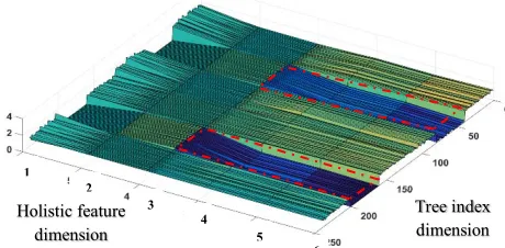
This is accumulated across all superpixels in the reference stereo image. The denominator in Eq. 4 ensures that remains normalized. The surface plot in Figure 3 shows Figure 3: A surface plot of the matrix A, used to weigh the

expert trees based on the holistic hand feature. A higher value indicates more weight. Consider a hypothetical holistic hand feature vector, [0, 0, 0, 1, 1, 1], which when post-multiplied with A will give less weighting to trees 40 to 80 and 160 to 200 based on their lower values (bluer colors).

Tree index dimension Holistic feature

dimension

6 5 3

2

how the different entries of A vary relatively. Figures 2 and 3 give an illustration of the weighting ability of A. The peaks indicate strong relationship between entries of h and the tree index. Studying both figures, consider a hypothetical example where = [0 0 0 1 1 1] . In this case, the holistic hand feature vector will weigh the prediction from the 240 trees based on the last three columns of , thereby giving less weighting to trees 40 to 80 and trees 160 to 200.

Let = [ , , … , ] ∈ ℝ( ∗ ) _{be a vector}

resulting from the concatenation of the actual probability distribution of all hand region superpixels and let =

, , … , ∈ ℝ( ∗ )× _{be the matrix whose row}

vectors are the concatenation of the predicted probability distribution from each tree. Then the unary potential in Eq. 4 can be rewritten for all superpixels in a single stereo image, z in matrix form as follows:

= 1 . (5)

The larger becomes, the more similar the consolidated predicted probability, , is to the true depth probability, .

Pairwise Potential: The pairwise potential enforces the constraint that adjacent superpixels often possess similar depth and hence similar probability distributions. This is based on the smooth nature of the depth of the hand surface. Similar to [13], a visual similarity measure between neighborhood superpixels is established to apply an adaptive depth similarity constraint. Specifically, neighbouring superpixels that appear dissimilar in terms of color, texture, and size will have a weaker pairwise potential encouraging similar predicted depth. This is particularly intuitive in a self-occluded scenario. The discontinuity in texture resulting from a finger occluding the palm, for example, will indicate that less smoothness constraint is placed on neighbouring superpixels that exist on the edge of the finger and the palm. To achieve this behavior, a similarity vector, , = , ( ), … , , ( ) , is

introduced,and a pairwise weighting, ∈ ℝ . For a pair of neighbouring superpixels, and , Q superpixel similarity measures are computed between them (more details on the superpixel similarity measures are presented in Section 5.2). We specify our pairwise potential as:

= 1

| | ,

( , )∈

, (6)

where U is a set of all possible pairs of neighbouring hand superpixels. Subsequently, the pairwise potential is a measure of the affinity of the probability of all pairs of neighbouring superpixels, and , determines the

contribution of each pair of superpixels to this measure. Let ∈ ℝ× _{be a matrix such that, its elements are given}

by

= , , (7)

and zeros everywhere else. is a D×D identity matrix. With this matrix, the pairwise potential in Eq. 6 can be represented in matrix form as:

= 1

| | . (8) A resulting depth image with high level of smoothness will yield a large pairwise potential, and vice versa.

Complete CRRF: At this stage, both potentials, unary and pairwise, have been established and that, the higher they are, the smoother and the more accurate the predicted depth becomes. Eqs. 3, 4 and 6 are combined to result in

Pr( | , ) = exp 1

+ 1

| | ,

( , )∈

, (9)

for a single stereo image pair. In this unified framework, the aim is to maximize Eq. 9 based on and . For all stereo images in the training set, z, the framework attempts to maximize ∑ log Pr ( ) ( ) _{. Formally,}

max

, log Pr

( ) ( ) _{+ (1 − ), (10)}

where is the decay weight on the constraint with maintaining a unit length and

log Pr( | , ) =1

+ 1

| | ,

( , )∈

. (11)

During optimization, we ensure that all the entries of are positive, so that represents a probability. With the aim of solving for Eq. 10, stochastic gradient ascent is applied using the partial derivative of Eq. 11 with respect to

and . log Pr( | , )

=1 ( ) −

[ ] (12)

and

{log Pr( | , )} = 1

| | , ( , )∈

. (13)

4.3.Prediction

Having established and , predicting the posterior probability for new stereo pairs involves solving the Maximum a Posteriori inference on Eq. 9. To achieve this, the matrix representations of and are used in Eq. 5 and Eq. 8 resulting in

Pr( | , ) = exp _{| |} + . (14) The aim is to determine that maximizes Pr( | ) for a pre-computed and pair.

∗_{= argmax Pr( | , ) = argmax}

| | +

(15) This is easily derived in closed form by solving for the zeros of the second derivative. Formally,

∗₌ | | _{. (16)} ∗_{represents the concatenated predicted depth probability}

for all superpixels in an image. The predicted depth level for a superpixel is the depth with the maximum depth probability.

5.Implementation Details

5.1.Registering reference stereo to RGBD camera

To establish a database of strong registration between the pairs of data, image and depth acquisition were carried out

on both the stereo camera and a RGBD camera, almost adjacently positioned. Using camera calibration [14], depth data from an RGBD sensor was registered to the left image of the RGB pair. This allows {( , )( )_{, … , ,} ( )_{} to}

be established for all captured instances of stereo pairs, z. 5.2.Extracted Features

Matching-cost Features, : our implementation used five matching cost functions: Sum of Absolute Difference (SAD), Sum of Squared Differences (SSD), Normalized Cross Correlation (NCC), Quantized Census (QC), and Zero-mean Sum of Absolute Differences (ZSAD). The reader is referred to [1] for details on these cost functions. These cost measures were chosen because of their prominence, computation cost and simplicity. Each of the cost functions were applied under three window sizes: [7 × 7], [11 × 11], and [15 × 15].

Holistic Hand Features, h: For each captured instance of stereo pairs three main factors are focused on in describing the scene. First, the average intensity value of all hand region pixels across all three-color channels is considered. This quantifies the skin tone. Second, the aggregative shift of all hand pixels in the reference stereo camera compared to the other stereo camera is computed. This quantifies how far away the hand is from the camera, representing the difference in the average pixel’s position for hand region pixels in both cameras. Last, we compute the ratio between the numbers of hand and non-hand region pixels. This

Re

fe

re

nce

Im

age

G

ro

und

Tr

ut

h

CRRF

(P

ai

rw

is

e

+

U

nar

y)

RRF

+

Un

ar

y

RRF

(w

it

h

Ho

list

ic

F

eat

ur

e) cm

SG

M

quantifies the size of the hand (if considered relatively to the aggregative shift). This analysis resulted in a six-dimensional holistic hand feature vector (3 color channels values, 2 vector shift values, and 1 ratio of pixels in the hand vs. non-hand regions).

Superpixel Similarity Measure, , : To quantify

similarities of two neighboring superpixels, four measures were used. The first measure is the difference in the average LAB color of both superpixels. The second is the difference in the Local Binary Pattern. The third measure is the difference in the standard deviation of pixels’ values in LAB color. Finally, we examine the summed difference in histogram. In each of these cases, the exponent of the negative Euclidean norm is applied to the resulting difference. For instance, the LAB difference is ( )_, =

|| ||_{, where is the average LAB value for}

superpixel . This yields a similarity measure vector with a length of four or = 4.

5.3.Data and Training

Using the setup described above, 500 instances of hand poses at different distances, from 12 different participants (6,000 stereo pairs in total), were captured. Participants were of different skin tone, hand size and gender. Data from four participants was reserved for testing, and the remaining data (from the other eight participants) was used for training. SLIC segmentation was applied to all reference stereo images, producing approximately 3,000 superpixels per image. Note that only a fraction of these 3,000 superpixels are hand region superpixels. The amount of hand superpixels (ranging approximately from 200 to 500 per image capture) depends on the distance between the hand and the camera. In total, roughly 2.5 million superpixels were used in training and evaluating the algorithm. The depth values posterior distribution of the RRF was quantized into 500 bins, i.e. D = 500. The depth range of the hand poses in the entire dataset, generally ranged from 500mm and 1800mm. Hence, the RRF can predict to a resolution of (1800mm-500mm)/500 bins = 2.6 mm. Each round of training (i.e., to train for each posterior

( )_{) takes approximately 3 - 4 hours. Since eight rounds}

were needed, training took roughly one day. Finally, the propagation of all superpixels and combining the posteriors using executes typically in 185 seconds. Hence testing for the depth, a frame of stereo images on the cluster will typically take 260 seconds.

5.4.Stochastic Gradient Descent

and are learned separately by first randomly initializing with all elements of A being positive. We trained for A and with the learning rate initialized at

12,000. We ran 100 epochs, reducing the learning rate by 10% every 10 epochs. The decay weight, λ, was set as 0.05.

6.Experimental results

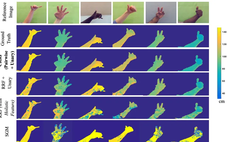
The approach was validated experimentally, presenting both qualitative (Figure 4) and quantitative (Table 1) results. Three main comparisons were made, these include: prediction solely using RF (with only matching-cost features and with a combination of matching-cost and holistic features); using RF with the unary term framework; as well as a prominent stereo-matching technique (SGM). The results were quantitatively appraised for accuracy by computing the percentage of correctly predicted depth both at superpixel and pixel levels,∑ {| | }, where and are the ground truth and the predicted depth at superpixel (or pixel) p; {} is a function that returns 1 for true input and 0 otherwise; and N is the number of hand region pixel/superpixel. We also computed the average relative error, ∑ | |, to quantitatively evaluate the performance of the test.

6.1.Stereo-matching Comparison

To validate the machine learning approach, we attempt to extract depth (through disparity) from stereo pairs in our dataset using a prominent stereo matching technique, SGM. At the time of writing, this was the 9th _{best performing} published stereo-matching technique on the Middlebury stereo evaluation chart [6]. We compare to SGM as it is the highest performing technique for which a MATLAB implementation is readily available.

We also compared the proposed method with [16], which also applies a regressive random forest to estimate image depth. However, in [16], a single similarity measure (Quantized Census) is used to compute a depth image, and no pairwise term is modelled in the regression that maps a disparity image to a depth image. As the results in Table 1 show, our method, even without the pairwise term, outperforms [16]. We attribute the improved performance of our CRRF method to the features used. Unlike [16], which uses a single similarity measure, our method learns the features that best regress the depth using multiple similarity measures, disparity shifts, and window sizes in a concatenated feature vector. Also unlike [16], which uses disparity as an intermediate representation, our CRRF method maps directly from the stereo pair to depth. Additionally, our approach to regression is more sophisticated in that we conditionally learn expert trees, which are combined using holistic hand features. Finally, the pairwise term in our model provides additional smoothing constraints that yield superior performance.

6.2.Baseline Comparison

Three baseline comparisons were made. The first was predicting depth solely from the matching-cost feature, using conventional RRF. The results (Figure 4 and Table 1) validate our hypothesis that applying a machine learning approach to determining stereo correspondence is a more effective approach. Using a set of simple stereo matching criteria and stochastically determining which to use at different tree depths has resulted in almost a 272.7% increase (from 0.132 to 0.492) in pixel level accuracy.

Secondly, we augmented the matching-cost feature by concatenating it with the holistic hand features whilst still regressing with a conventional RRF model. The aim was to specifically investigate the impact of using “expert trees”. From Table 1 we can see a notable improvement in the prediction resulting from adding the holistic feature, yielding greater accuracy (0.492 to 0.689) and less relative error (0.500 to 0.353) in both superpixel level and pixel level. However, a much greater increase in accuracy results from using the holistic feature to learn expert trees as

opposed to just concatenating it with the stereo-matching feature. This yielded a 50.2% increase in accuracy on average in comparison to the 29.1% increase in accuracy provided by solely concatenating the holistic features.

The last baseline comparison was to investigate the significance of the pairwise term. Recall that the contribution of the pairwise term is to add a smoothing constraint on the depth prediction. This is presented in the qualitative results. The predicted depth is clearly smoother and hence a better representation of the surface of the hand. The quantitative result from Table 1 also conveys the superiority of the prediction made when the pairwise term is applied. Interestingly, the pixel level accuracy is almost as strong as the superpixel level accuracy when the pairwise term is applied. This is again due to the smoothing effect.

7.Conclusion

In this paper, we proposed and developed an innovative application of the regression forest technique for resolving depth from stereo images. We present Conditional Regressive Random Forest, a framework that uniquely combines expert trees based on the features of the superpixel whose depth is being predicted. Note that the technique is relevant for to other applications, including classification problems like scene labelling. The framework further enforces smoothness constraints as it predicts depth of superpixels away from the camera. Thus, we have demonstrated the use of a relatively cheap stereo camera rig to generate a high-quality depth image of the hand.

RGB cameras have advantages over depth cameras as discussed in the introduction, but computing the depth of a hand using standard stereo algorithms that use a single matching cost function produces inferior results due to ambiguities arising from a lack of texture, and variations in hand size and skin tone. To date, the use of machine learning for hand depth estimation has received little attention, despite the importance of depth estimation for hand gesture and pose estimation in HCI applications. This paper fills this gap by presenting a new state-of-the-art machine learning approach in recovering accurate depth images from stereoscopic images of the hand.

Methods Superpixel Level Accuracy Pixel Level Accuracy Ave. Relative Error

t=10mm t=20mm t=10mm t=20mm per Superpixel per Pixel

SGM [11] - - 0.103 0.132 - 0.772

Basaru et al. [16] - - 0.455 0.515 - 0.534

RRF 0.599 0.610 0.423 0.492 0.503 0.500

RRF (with Holistic Feature)

0.686 0.757 0.610 0.689 0.358 0.353

RRF + Unary 0.835 0.885 0.684 0.788 0.229 0.231

CRRF (Pairwise + Unary)

0.911 0.911 0.811 0.852 0.181 0.190

References

[1] Basaru, R., Alonso, E., Child, C., and Slabaugh, G., (2014). Quantized Census for Stereoscopic Image Matching. In Proc. of the 3DV Conference: Workshop, Dynamic Shape Measurement and Analysis. Dec 2014. [2] https://www.leapmotion.com/ [Accessed 17th _October

2016]

[3] Shotton, J., Fitzgibbon, A., Cook, M., Sharp, T., Finocchio, M., Moore, R., Kipman, A., and Blake, A. (2011). Real-Time Human Pose Recognition in Parts from Single Depth Images. In Proc. of the IEEE Conference on Computer Vision and Pattern Recognition. June 2011.

[4] https://www.oculus.com/ [Accessed 17th _October 2016]

[5] Fanello S., Keskin C., Izadi S., Kohli P., Kim D., Sweeney D., Criminisi A., Shotton J, Kang S.B., and Paek T.,(2014) Learning to be a Depth Camera for Close-Range Human Capture and Interaction. In the Journal of ACM (Association for Computing Machinery) Transactions on Graphics, Volume 33 (4). [6] http://vision.middlebury.edu/stereo/data/ [Accessed

28th April 2015]

[7] Phung, S., Bouzerdoum, A., and Chai, D., (2005). Skin Segmentation Using Color Pixel Classification: Analysis and Comparison. In the IEEE Transactions on Pattern Analysis and Machine Intelligence, Volume 27 (1).

[8] Hasan, M.M.,and Mishra, P.K. (2012). Superior Skin Color Model using Multiple of Gaussian Mixture Model. In the British Journal of Science, Volume 6 (1). [9] Sun, M., Kohli, P., and Shotton, J. (2012). Conditional Regression Forests for Human Pose Estimation. In Proc. of the IEEE Conference on Computer Vision and Pattern Recognition. June 2012.

[10]Payet, N., and Todorovic, S., (2010) Random Forest Random Field. In Proc. of the Advances in Neural Information Processing Systems. June 2010.

[11]Hirschmuller, H. (2005). Accurate and Efficient Stereo Processing by Semi-Global Matching and Mutual Information. In Proc. of the IEEE Conference on Computer Vision and Pattern Recognition. June 2005. [12]Murphy K.P. (2012) Machine Learning – A

Probabilistic Perspective. Cambridge: MIT Press. [13]Liu F., Gould S. and Shen C. (2014). Deep

Convolutional Neural Fields for Depth Estimation from a Single Image. In Proc. of the IEEE Conference on Computer Vision and Pattern Recognition. June 2014.

[14]Zhang, Z. (1999). Flexible Camera Calibration by Viewing a Plane from Unknown Orientations. In Proc. of the International Conference on Computer Vision. September 1999.

[15]Grzeszczuk R., Bradski G., Chu M.H., and Bouguet J.Y. (2000). Stereo Based Gesture Recognition Invariant to 3d Pose and Lighting. In Proc. of the IEEE Conference on Computer Vision and Pattern Recognition. June 2000.

[16]Basaru, R., Alonso, E., Child, C., and Slabaugh, G., (2016). HandyDepth: Example-based Stereoscopic Hand Depth Estimation using Eigen Leaf Node Features. In Proc. of the IWSSIP International Conference. May 2016.

[17]Dantone M., Gall J., Fanelli G., Van Gool L. (2012). Real-time Facial Feature Detection using Conditional Regression Forests. In Proc. IEEE Conference for Computer Vision and Pattern Recognition. June 2012. [18]Liu B., Gould S. and Koller D. (2010). Single Image

Depth Estimation from Predicted Semantic Labels. In Proc. IEEE Conference for Computer Vision and Pattern Recognition. June 2010.

[19]Saxena A., Chung S.H. and Ng A. Y. (2005). Learning Depth from Single Monocular Images. In Proc. of the Advances in Neural Information Processing Systems. 2005.

[20]Saxena A., Chung S.H. and Ng A. Y. (2009). Make3d: Learning 3d Scene Structure from a Single Still Image. In the IEEE Transactions on Pattern Analysis Machine Intelligence, Volume 31 (5).

[21]Eigen D., Puhrsch C., and Fergus R. (2014). Depth Map Prediction from a Single Image Using a Multi-Scale Deep Network. In Proc. of the Advances in Neural Information Processing Systems. Dec 2014. [22]Oikonomidis I., Kyriazis N., and Argyros A.A. (2011).

Full Dof Tracking of a Hand Interacting with an Object by Modelling Occlusions and Physical constraints. In Proc. of the IEEE Conference on Computer Vision and Pattern Recognition. June 2011.