M E T H O D O L O G Y
Open Access
Detecting gene-gene interactions using a
permutation-based random forest method
Jing Li
1, James D. Malley
2, Angeline S. Andrew
3, Margaret R. Karagas
3and Jason H. Moore
4,5**Correspondence: [email protected] 4Institute for Biomedical Informatics, University of
Pennsylvania, Pennsylvania, PA, USA 5Department of Biostatistics and Epidemiology, The Perelman School of Medicine, University of Pennsylvania, Pennsylvania, PA, USA Full list of author information is available at the end of the article
Abstract
Background: Identifying gene-gene interactions is essential to understand disease susceptibility and to detect genetic architectures underlying complex diseases. Here, we aimed at developing a permutation-based methodology relying on a machine learning method, random forest (RF), to detect gene-gene interactions. Our approach called permuted random forest (pRF) which identified the top interacting single nucleotide polymorphism (SNP) pairs by estimating how much the power of a random forest classification model is influenced by removing pairwise interactions.
Results: We systematically tested our approach on a simulation study with datasets possessing various genetic constraints including heritability, number of SNPs, sample size, etc. Our methodology showed high success rates for detecting the interaction SNP pair. We also applied our approach to two bladder cancer datasets, which showed consistent results with well-studied methodologies, such as multifactor dimensionality reduction (MDR) and statistical epistasis network (SEN). Furthermore, we built
permuted random forest networks (PRFN), in which we used nodes to represent SNPs and edges to indicate interactions.
Conclusions: We successfully developed a scale-invariant methodology to detect pure gene-gene interactions based on permutation strategies and the machine learning method random forest. This methodology showed great potential to be used for detecting gene-gene interactions to study underlying genetic architectures in a scale-free way, which could be benefit to uncover the complex disease mechanisms.
Keywords: Random forest, GWAS, Machine learning, Scale invariant
Background
Genome-wide association studies (GWASs) have revolutionized the strategy for identi-fication effects of single nucleotide polymorphisms (SNPs) on disease susceptibility and detecting genetic architectures underlying complex diseases from large-scale genotyp-ing data, such as type II diabetes, obesity and cancer [1–5]. GWASs have uncovered a great number of disease susceptibility loci, yet we still have very limited knowledge of the genetic architecture of some diseases and therefore cannot accurately predict the disease risk from genetic information [6]. This is challenging due to the consequences of genetic heterogeneity, epistasis (gene-gene interactions) and gene-environment interactions. Tra-ditional methods that have been used to analyze the genetic-disease associations include linear regression, logistic regression, chi-square test, etc. However, these approaches map single loci one at a time to detect main effects, but ignore interactions between
genes and environment factors when mapping the relationship between genotypes and phenotypes [4, 6, 7].
As an alternative to commonly used linear models and other classical methods as above, we applied data mining and machine learning methods, such as multifactor dimension-ality reduction (MDR), artificial neural network (ANN) and statistical epistasis network (SEN), etc., to detect interactions between different genes, and between genes and envi-ronmental exposures during modeling. The concept here is that these methods perform better to capture the non-linear mapping from genotypes to phenotypes [4, 8–11]. Multi-locus analysis methods, however, can sometimes be computationally challenging when examining all pairwise combinations of SNPs [7]. It can get even more computationally challenging when trying to detect three-way or four-way interactions [7]. Different strate-gies have been designed to solve such problems, which include applying filter algorithms to reduce the number of SNPs in the analysis by removing redundant SNPs based on the needs, such as Spatially Uniform ReliefF (SURF), and doing pathway analysis to subset the SNP dataset based on similar biological functions [12, 13].
One class of widely used algorithms in machine learning are tree-based methods, such as decision trees (DTs) and random forests (RFs), which belong to the supervised machine learning methods that are used for variable selection, classification and outcome predic-tion [14]. A single DT grows according to a best binary splitting rule which splits data into two subgroups at each node [15]. For GWAS studies, DT is generated by selecting the best SNP predictor as the node where it best separates samples into two groups; the selection occurs at each further node until, in the default mode, the DT is grown to purity (fully separation of the two classes at the terminal nodes), or until a small number of samples are left at the terminal nodes, to avoid over-fitting [15]. However, purity default method is itself known to overfit. Once the DT is fully learned using training data, the testing data is then applied to the DT by dropping prediction variable values (SNP genotypes) down the tree. DT could output either the predicted class label of the sample based on the most frequent class DT predicts, or quantitatively predicts the mean of the outcomes using regression DTs [14]. In regression mode, the DT uses a local average of the outcome values in each terminal node. RF extends the idea of DTs, a nonparametric tree-based method that uses bootstrap sampling to build an ensemble of DT classifiers and predicts the outcome by aggregate voting from all DTs [16, 17]. Usually, the number of trees and how many splitting rule would apply at each node are used to tune the RF [14].
forest approach, sliding window sequential forward feature selection (SWSFS) algorithm, to detect epistatic interactions in case-control studies according to gini importance [23].
Although RF implicitly considers interactions, further work is required to separate main effects from interactions in RF since VIMs as estimated in RF reflect both main and inter-action effects [24, 25]. Unfortunately, previous work has shown that RF is not designed to explicitly test for SNP interactions with hypothesis tests in large genetic datasets, due to the decreasing probability of the co-ocurrence of SNPs predictors in each tree as the feature space is expanded [25]. Therefore, modeling needs to be done carefully to detect interactions and new methodologies need to be designed to capture the pure interactions without main effects between SNPs when modeling with RF.
In this study, we proposed an approach called permuted random forest (pRF) to detect pure interactions between SNPs, which included four steps: training, permutation, testing and ranking. Random forest was trained using original dataset and for each pairwise of SNPs, dataset was later permuted using two methods: one permutation method kept the main effects of the chosen pair of SNPs, the other method kept the main effects and inter-action of the chosen pair of SNPs. The subtrinter-action of the two schemes was defined here as the interaction signal between the chosen SNP pair, and therefore measures how different RF outcomes were due to how much the interaction signal contributes to the prediction models. We hypothesized that if two SNPs are highly interacting with each other, the success rate for RF to classify the samples correctly would be affected greatly when remov-ing the interaction between the two SNPs. The stronger interactive SNPs could then be identified by ranking the different classification errors from the above two permutation schemes. We tested our hypothesis systematically on simulated datasets obtained from Genetic Architecture Model Emulator for Testing and Evaluating Software (GAMETES) with different genetic constraints including heritability, number of SNPs, sample size, etc, and achieved good success rates on detecting the interacting SNP pairs even under very low heritabilities. We also applied our approach on two real bladder cancer datasets: one was a 7-SNP dataset with a single pair of SNPs had interaction, the other was a 39-SNP dataset with multiple pairs of SNPs had interaction. We were able to replicate previously identified interacted SNPs by two well-studied methods, MDR and SEN, and also made evidently new discoveries on SNPs with interactions. Finally, we introduced the idea of permuted random forest networks (PRFN), in which we used nodes to represent SNPs and edges to indicate interactions.
Methods
Permuted random forest (pRF)
were generated from two permutation schemes as shown below. For each pair of SNPs, one testing dataset had its interaction deleted, while the other testing dataset kept the interaction between this pair of SNPs. Thus, the difference of the two testing datasets was purely the interaction, and the different prediction error rate was caused by the existing interaction between this pair of SNPs.
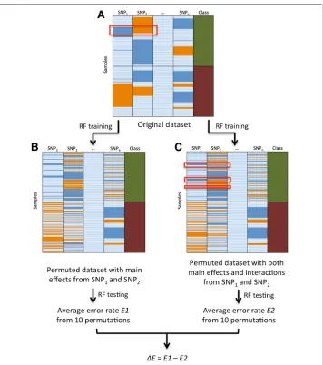
Our approach consisted of four steps of (1) training, (2) permutation, (3) testing and (4) ranking using machine learning algorithm RF. In the first step training, RF was trained using the whole original SNPs dataset. We used‘randomForestSRC’package in R with the settingsnsplit=0,ntree=100and the rest as default, which was a well-established pack-age for carrying out random forest analysis for survival, regression and classification [26]. The RF structure from the training stage was retained, and the structure was later be used for testing on the permuted datasets. The original dataset was shown in Fig. 1a, each col-umn in the dataset represented a SNP while the last colcol-umn represented the phenotypes; each row represented a sample.
In the second step of permutation, for each pair of SNPs independently, we carried out two permutation strategies to generate two testing datasets. The difference between the two testing datasets was merely the preservation or deletion of the interaction between the pair of SNPs. Previously, Greene et al. designed an explicit test of epistasis to remove SNP interactions, which was based on a permutation method [27]. In their approach, data rows were sorted by class into cases and controls, permutations were then performed in each column within each class to remove any interactions between SNPs in each class [27]. The independent main effects of SNPs were preserved due to the consistent genotype frequencies within each class before and after the permutation [27]. Our two permuta-tion frameworks were motivated from Greene’s method. In our first permutapermuta-tion strategy, data rows were sorted by class into cases and controls, one pair of SNPs were selected and both of their genotypes (0, 1 or 2) were shuffled within each class. By doing this, the interaction between the two SNPs was removed, but the main effects from the two SNPs were maintained. In our second permutation strategy, the same two SNPs were permuted by maintaining their interactions and main effects. In more detail, data rows were sorted by class into cases and controls, and their genotypes (0, 1 or 2) were shuffled together by keeping the combination of SNP information within each class. As shown in Fig. 1a and c, the interaction pattern between SNP1and SNP2, indicated inside red rectangles by
the blue-orange pattern, was consistent before and after our second permutation strat-egy. For each pair of SNPs, the above two permutation frames were repeatedly applied to generate two testing datasets. It is also worth mentioning that the interactions among other non-selected SNPs were preserved in both of the permutation frameworks since all the SNPs were considered for the model. This is an advantage of our method since other interactions may have direct or indirect effects on the selected SNPs.
Fig. 1Overview of the permuted Random Forest (pRF). Shown in panelais the original dataset with all the SNP information (0, 1 or 2) and class (cases-control status). Each row represents a sample; different three colors in the SNP columns indicate different genotypes, and two colors in the class column indicate case-control status.bshows the first permutation framework that keeps SNPs’ main effects, in which cases and controls are separated, two selected SNP columns shuffle the information separately within each class.cshows the second permutation framework that keeps SNPs’ interaction and main effects, in which cases and controls are separated, two selected SNPs shuffle their information together by keeping their genotype combinations, separately within each class. RF is trained using original dataset and tested using the datasets from the above two permutation schemes. Error rates are calculated by averaging the classification errors across all samples. The same process is repeated 10 times and the error rates are averaged from 10 permutation results. The average classification error from the first permutation framework is namedE1, while the average classification error from the second permutation framework is namedE2. The whole process is repeated on all pairs of SNPs and the difference in average error rates (E = E1 - E2) are calculated and ranked to identify the top candidates
In the last step, after each pair of SNPs independently was permuted using the above two permutation schemes and tested to get the prediction errors, the error rate differ-ence (E=E1−E2) was calculated for each pair of SNPs. TheEwas used to define the strength of the interaction exists, since omitting a strong interaction could have a strong affect on classification power. The larger theEwas, the stronger interaction sig-nal was indicated for that pair of SNPs. TheEs were ranked and the pair of SNPs with the largestEhaving the strongest interaction among all SNPs, or we could identify the top interactive SNPs given a particular threshold. For simulation studies, the same pro-cess was repeated on the 100 replicate datasets in order to calculate the overall sucpro-cess rate of interaction detection using our approach.
Multifactor dimensionality reduction (MDR)
Multifactor dimensionality reduction (MDR) is a very popular method that can accurately identifies gene-gene and gene-environmental interactions, which is nonparametric and model-free [8, 28]. To carry out an MDR analysis, a group of n genetic attributes or envi-ronmental factors are first selected from all provided factors as the model. All possible combination of the n factors are then represented in the n-dimensional space. The ratios of cases vs. controls are calculated in each condition of the n-factor combinations. The n-dimensional space could be reduced to one dimensional following the grouping rule: the spaces that have the number of cases more than controls are classified as higher risk group, while the spaces that have the numbers of controls more than cases are classified as lower risk group [8, 28]. The classification method can then be used on on this single variable at the reduced dimension space. Traditionally, MDR uses 10-fold cross validation. For each cross validation training set, models are ranked using balanced accuracy. The number one ranked model is the winner for this round. After the 10 rounds, the model with the plurality of wins across the training datasets is the overall winner for that model size. MDR has a lot of advantage. It reduces the dimensionality to one thus makes it eas-ier for the later classification. It is non-parametric, where no parameters are estimated, which is a big advantage over lots of traditional parametric statistical methods. It is also model-free, where no genetic model is assumed and thus give it great utilization on study-ing the disease where no inheritance-model is known for that or those models are very complicated [8, 28]. Over the past decade, a lot of method and tools has been contribut-ing to MDR to make it use more widely, such as a lot of filter approach to MDR, and a lot of wrapper approaches [29].
Statistical epistasis network (SEN)
Genome-scale integrated analysis of gene networks in tissues (GIANT)
Genome-scale Integrated Analysis of gene Networks in Tissues (GIANT) is a user friendly interface which provides the interactive visualization of the tissue specific networks [30]. The genome-wide functions interaction networks were built from a collection of datasets that covers thousands of experimental results that were extracted from more than 14,000 different publications [30]. The 144 tissue or cell lineage specific contexts were selected across the datasets and network-wide association study (NetWAS) was also developed to analyze the functional networks [30]. This could tremendously helpful to study human disease since most of the human diseases are the result of the gene interactions happened within a particular cell lineage or tissue. Carrying out the network in a tissue specific specific way could increase the accuracy of the results.
Genetic architecture model emulator for testing and evaluating software (GAMETES) Genetic Architecture Model Emulator for Testing and Evaluating Software (GAMETES) is a user-friendly software designed by Urbanowicz et al. for simulation studies [31]. GAMETES can generate random, pure and strictn-locus models. Pure models are defined asno single locus displays a marginal effectand strict models refer tono subset of the n-locus are predictive of phenotype information[32]. Such a simulation scheme is preferred here, since more traditional methods are computational expensive and, more impor-tantly, are unlikely to yield pure and strict epistasis models, as defined above. Specifically, GAMETES generates models using specified genetic constraints, and these can include the choice of different heritabilities, minor allele frequencies and population preva-lence [31]. Data and models constructed this way can also be ranked by the relative ease of detection metric (EDM), a score that is calculated directly from the model itself, and can lead to further generation of models based on the needs of simulation studies [33]. In this regard, it is notable that GAMETES also involves a data simulation strategy which can quickly and easily generate an archive of simulated datasets for each given model, which, in turn is helpful for further simulation studies [31]. In addition, different sample sizes are later selected when models are used to generate an archive of simulated datasets.
RandomForestSRC
“RandomForestSRC” is a R package developed for doing survival, regression and classi-fication using machine learning method random forest. Survival forests can grown for right-censored survival data, while regression and classification forests can grown based on either categorical or numeric response [26]. Splitting rules could be selected by users as deterministic or random. Variable selection is implemented by minimal depth variable selection [26]. This package also has the function of the imputing missing data, however, to keep the results comparison consistently we did not use this function in our analy-sis. This package could runs in both serial and parallel modes, which could be chosen by users [26].
Datasets
Simulated study design
Hence for this purpose, epistatic 2-locus SNP-disease models and an archive of datasets for each given model were generated using the GAMETES. Specifically, GAMETES was used to generate 100,000 random, strict and pure genetic models for each of 8 differ-ent combinations of genetic constraints that are differed by number of locus (SNPs) of 2, heritabilities of 0.001, 0.005, 0.01, 0.05, 0.1, 0.2, 0.3 or 0.4, minor allele frequency (MAF) of 0.2 and population prevalence that is allowed to vary. For each of the 8 genetic con-straints combinations, 100,000 models were ranked by EDMs and the models with the highest and lowest EDMs were selected as the two models for data simulation [33]. For each selected model, we simulated 100 replicate datasets under the sample size 2,000 or 4,000 with balanced cases and controls and using different total numbers of SNPs 5, 10, 15, 20 and 25. All together, we generated a total of 16,000 (8 (heritabilities)×2 (EDMs) ×2 (sample sizes)×5 (number of SNPs)×100 (replicates)) datasets, which were used for method evaluation. Each dataset contained one pair of highly interacted SNPs, named
M0P0,M1P1, and the rest of SNPs were namedNx. We calculated the success detection rate of our method pRF by observing how often the datasets among the 100 datasets lead to detection of the interacting SNP pair,M0P0andM1P1.
7-SNP bladder cancer dataset
The cases in the dataset were selected from people who were diagnosed with bladder cancer among those between 25–74 years old and from July 1994 through June 1998 in the New Hampshire State Cancer Registry. Controls were chosen from population lists in New Hampshire Department of Transportation (age≥65), population lists in Cen-ters for Medicare & Medicaid Services (CMS) of New Hampshire (age < 65), shared controls from a non-melanoma skin cancer study with diagnostic period of July 1993 to June 1995, and with additional controls assigned to match the cases on age and gender [34]. Informed consent was obtained from all participants. To collect the sam-ples, DNA was isolated usingQiagen genomic DNA extraction kits(QIAGEN Inc.) from peripheral circulating blood lymphocyte specimens, and genotyping was performed using SNP mass-tagging system from Qiagen Genomics and PCR-RFLP. Dataset was prepro-cessed based on the sufficient DNA concentration and successful genotyping, and the missing phenotypes/genotypes were imputed using the corresponded most frequent phe-notypes/genotypes. In this study, we selected a subset of 7 SNPs that had been previously identified to include a highly interacted SNP pair from this data. This dataset includes 560 controls and 354 bladder cancer cases after pre-processing. This dataset had one pair of SNPs had interaction.
39-SNP bladder cancer dataset
a previous SNP-SNP interaction study [10]. The 39 SNPs have previously been identified as the largest connected components with interactions in the statistical epistasis network (SEN) [10]. This dataset includes 791 controls and 491 bladder cancer cases. This dataset had multiple pairs of SNPs had interactions.
Results
Evaluation of our method using simulated data
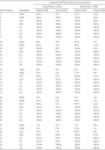
A total of 160 different datasets, each with 100 replicates were simulated using GAMETES based on the different combination of genetic constraints, that included number of inter-action locus (2), heritability (0.001, 0.005, 0.01, 0.05, 0.1, 0.2, 0.3 or 0.4), minor allele frequencies (0.2), number of SNPs (5, 10, 15, 20 or 25), sample size (2000 or 4000), extreme EDM (highest or lowest) and population prevalence that is allowed to vary. The datasets were generated from random, pure and strict epistasis models using GAMETES, with one pair of highly interacted SNPs namedM0P0,M1P1, and with the rest of SNPs namedNx. The success rates for identifying the interacting SNPs,M0P0andM1P1, were calculated for each dataset, and averaged from 100 replicates; see Table 1. It was shown that under most of the genetic constraint combinations, our approach achieved great success rates when identifying interacting SNPs. We also observed that our approach performed bet-ter when detecting inbet-teraction in models with the highest EDM and higher heritability, in datasets that include less numbers of SNPs, or larger sample size. For the datasets with 5 SNPs, the success rates were 100 % for all the datasets with heritability greater or equal to 0.05.
Evaluation of our method using 7-SNP bladder cancer dataset by comparing with MDR The subset of bladder cancer dataset contained 7 SNPs, XRCC3 (rs861539),
APE1 (rs3136820), XPD_751(rs13181), XRCC1_399(rs25487), XPD_312 (rs1799793),
XRCC1_194(rs1799782),XPC_PAT(rs2228001). We applied our permuted Random For-est (pRF) on this dataset and successfully identified the SNP pair,XPD_751andXPD_312, with the highest different error rates using our two permutation schemes. RF was applied on the whole dataset using R package‘randomForestSRC’with the default setting except
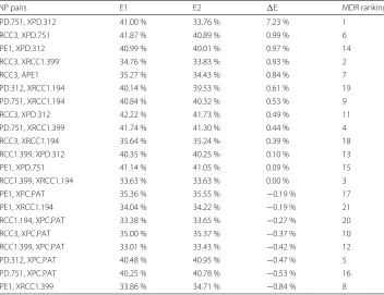
nsplit=0,ntree=100. The same two permutation strategies were used and repeated 10 times to obtain the average error rate differenceEfor each pair of SNP. As shown in Table 2, by removing the interaction between this two SNPs using permutation strategy, the error rate was greatly increased from 33.76–41.00 %.Ewas 7.23 % for this SNP pair, while the rest ranged from−0.84–0.99 %. Different numbers of permutations, tree num-bers and splitting rules had been applied in our method; however, the interaction pair could always be identified (data not shown). To compare our method with other method, MDR was also used on the same dataset to identify the top 2-way models, which indicates the highly interacted SNPs. The last column showed how the MDR ranks the top 2-way models based on the likelihood of having interactions among the SNPs. We found for the most interacted pair shown by our approach, MDR was showing the consistent results by ranking it as the most interactive pairs of SNPs as well.
Table 1Success rates for identification of interaction pairs of SNPs from simulation studies Interaction SNP Pair Detection Success Rate
Sample Size=2000 Sample Size = 4000
SNP Numbers Heritability Highest EDM Lowest EDM Highest EDM Lowest EDM
5 0.001 52 % 7 % 70 % 16 %
5 0.005 99 % 28 % 100 % 43 %
5 0.01 100 % 34 % 100 % 68 %
5 0.05 100 % 100 % 100 % 100 %
5 0.1 100 % 100 % 100 % 100 %
5 0.2 100 % 100 % 100 % 100 %
5 0.3 100 % 100 % 100 % 100 %
5 0.4 100 % 100 % 100 % 100 %
10 0.001 8 % 3 % 29 % 1 %
10 0.005 80 % 4 % 99 % 13 %
10 0.01 100 % 8 % 100 % 43 %
10 0.05 100 % 98 % 100 % 100 %
10 0.1 100 % 100 % 100 % 100 %
10 0.2 100 % 100 % 100 % 100 %
10 0.3 100 % 100 % 100 % 100 %
10 0.4 100 % 100 % 100 % 100 %
15 0.001 6 % 0 % 8 % 0 %
15 0.005 51 % 2 % 77 % 6 %
15 0.01 93 % 4 % 100 % 12 %
15 0.05 100 % 92 % 100 % 100 %
15 0.1 100 % 100 % 100 % 100 %
15 0.2 100 % 100 % 100 % 100 %
15 0.3 100 % 100 % 100 % 100 %
15 0.4 100 % 100 % 100 % 100 %
20 0.001 0 % 0 % 2 % 1 %
20 0.005 10 % 2 % 39 % 3 %
20 0.01 49 % 0 % 93 % 12 %
20 0.05 100 % 70 % 100 % 98 %
20 0.1 100 % 100 % 100 % 100 %
20 0.2 100 % 100 % 100 % 100 %
20 0.3 100 % 100 % 100 % 100 %
20 0.4 100 % 100 % 100 % 100 %
25 0.001 1 % 0 % 1 % 0 %
25 0.005 2 % 0 % 10 % 1 %
25 0.01 15 % 1 % 44 % 2 %
25 0.05 99 % 30 % 100 % 87 %
25 0.1 100 % 87 % 100 % 100 %
25 0.2 100 % 99 % 100 % 100 %
25 0.3 100 % 100 % 100 % 100 %
25 0.4 100 % 100 % 100 % 100 %
Success rates for identification of interaction pairs of SNPs with different numbers of SNPs, heritabilities, models with
highest/lowest EDMs, under the sample sizes of 2000 or 4000 with balanced cases and controls. The success rates were calculated using 100 replicate datasets. The percentage was calculated as the fraction of correctly detection times of the interacting SNP pair,M0P0andM1P1, in 100 replicate datasets under each genetic constraint combination of number of SNPs (5, 10, 15, 20 or 25), heritability (0.001, 0.005, 0.01, 0.05, 0.1, 0.2, 0.3 or 0.4), extreme EDM (highest or lowest) and sample size (2000 or 4000)
Table 2SNP interactions identified by permuted random forest (pRF)
SNP pairs E1 E2 E MDR ranking
XPD.751, XPD.312 41.00 % 33.76 % 7.23 % 1
XRCC3, XPD.751 41.87 % 40.89 % 0.99 % 6
APE1, XPD.312 40.99 % 40.01 % 0.97 % 14
XRCC3, XRCC1.399 34.76 % 33.83 % 0.93 % 2
XRCC3, APE1 35.27 % 34.43 % 0.84 % 7
XPD.312, XRCC1.194 40.14 % 39.53 % 0.61 % 19
XPD.751, XRCC1.194 40.84 % 40.32 % 0.53 % 9
XRCC3, XPD.312 42.22 % 41.73 % 0.49 % 11
XPD.751, XRCC1.399 41.74 % 41.30 % 0.44 % 4
XRCC3, XRCC1.194 35.64 % 35.24 % 0.39 % 18
XRCC1.399, XPD.312 40.35 % 40.25 % 0.10 % 13
APE1, XPD.751 41.14 % 41.05 % 0.09 % 15
XRCC1.399, XRCC1.194 33.63 % 33.63 % 0.00 % 3
APE1, XPC.PAT 35.36 % 35.55 % −0.19 % 17
APE1, XRCC1.194 34.04 % 34.22 % −0.19 % 21
XRCC1.194, XPC.PAT 33.38 % 33.65 % −0.27 % 20
XRCC3, XPC.PAT 35.00 % 35.37 % −0.37 % 10
XRCC1.399, XPC.PAT 33.01 % 33.43 % −0.42 % 12
XPD.312, XPC.PAT 40.48 % 40.95 % −0.47 % 5
XPD.751, XPC.PAT 40.25 % 40.78 % −0.53 % 16
APE1, XRCC1.399 33.86 % 34.71 % −0.84 % 8
Classification error rates from datasets obtained by two permutation schemes,E1(with main effects only) andE2(with main effects and interaction), are shown in the table. Error rate differences were calculated and listed asE. SNP pairs were ranked by their error rates differences in percentage, indicating the strength of interactions.SNP pairscolumn shows the permuted SNP names.MDR rankingcolumn shows the ranking of top 2-way models MDR identified according to the results from our approach
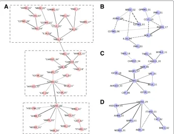
Fig. 2Statistical epistasis network (SEN) and permuted random forest networks (PRFN).ashows the largest connected components from statistical epistasis network, which includes 39 SNPs. The largest connected components were divided into three clusters. Permuted Random Forest (pRF) was applied using the SNPs within each of the three clusters separately.b,canddshow the PRFNs built from each cluster. The width of the edges are in proportion to how strong the interactions exist, which are represented by the differences in error rates using our method. The cut-off for the SEN was based on entropy value of 0.013. PRFNs were built using same numbers of edges as in each cluster in SEN
We further characterized the newly identified interactions using Genome-scale Inte-grated Analysis of gene Networks in Tissues (GIANT). As shown in Fig. 3, interactions between genesCCL5andPARP4in panel A,MBD2andGSTMin panel B,BCL6andXPC
in panel C were characterized usingGIANT with network filters set asminimum rela-tionship confidenceequals to 0.8 andmaximum number of genesequal to 5. By comparing our method to SEN, we concluded the difference was reasonable.
Discussion
GWAS provides a powerful approach to discover disease associated genetic variants and a lot of diseases associated SNPs have been discovered via GWAS, yet, that knowledge is still not enough to explain complex diseases [4]. By realizing that most genetic factors function in a complex mechanism when they interact with other genetic and environmen-tal factors, more methods and software packages focusing on detecting the interactions have been used [35]. Early methods to detect interactions include the logistic regression model with interaction terms, joint tests of association and exhaustive searches, but, with good reason, those methods are usually criticized for their inability to deal with high dimensional data [35]. Machine learning and data-mining methods have been developed lately, that use a space of possible models and avoid exhaustively searching the interac-tions [35, 36]. In our approach, we chose a popular machine learning method, random forest, which naturally considers interactions due to its DT structure. All those advan-tages make RF a suitable method to use in our strategy. Our rationale is that, if allowing the interaction between a particular SNP pair could increase the power to classify the samples using RF, the more the power increases, the stronger the interaction for that SNP pair. Therefore, we designed two different explicit permutation strategies thus to quanti-tatively characterize the interactions. In summary, we designed a new methodology based on combining both permutation methods and a machine learning method RF to capture gene-gene interactions.
To discuss our result for the simulation study, we found the success rates of our method to detect highly interacted SNP pairs were decreased as the number of SNPs in the dataset increased. For instance, we observed the success rates to be 70 and 30 % under the low-est EDM model at the number of SNP 20 and 25. However, when the sample size was increased from 2000 to 4000, it compensated for the difficulty of detection using datasets with lowest EDM models or the larger SNP size, which improved the ability to detect the interaction pair of SNPs. This was due to the nature of RF when the feature space gets expanded, and it was more generally of the problem of high dimensional data with sparse signal. Also, because this was a permutation-based method, when as the SNP size increased, it took much longer time to sort through all pairwise combinations. However, using parallel mode and running on clusters could help resolve this issue. On the 7-SNP bladder cancer dataset which we compared our result with MDR, we found the most inter-acted pair shown by our approach was the same as MDR as shown in the “Results” section. We look further for biological functions,XPDwas found to possess DNA repair capacity (DRC) and studies have found two XPD polymorphisms,XPDAsp312Asn and Lys751Gln, had a modulating effect on DRC and there existed possible association between XPD
Asp312Asn and Lys751Gln polymorphisms in lung cancer [37, 38]. All those biological evidence showed that our results are reasonable. We think that our methodology could correctly detect the pair of SNP that has interactions in a dataset containing one pair of interactive SNPs.
in three clusters in Fig. 2b–d comparing to SEN. Beside those overlapping interactions, we also identified new SNP-SNP interactions that were relatively strong, which included
MBD2_02(rs1145315) andGSTM3_01,MBD2_02andAXIN2_02. To further check the biological functions,MBD2was methl-CpG-binding domain protein 2, which belonged to methyl-CpG-binding domain (MBD) and had been previously identified possessing the function of activating certain promoters by de-methylation, particularly in cancer [39].
GSTM3had been found to play a role in detoxification of carcinogens and modulating cancer susceptibility [40]. Based on those biological facts, we think that those two genes may highly be likely to act together in causing cancer. Besides the overlapping interac-tions and new discovered interacinterac-tions, there were also some nodes missing in our network comparing to SEN. We think this may be caused by missing some SNP nodes due to the cut-off we chose, since we were choosing the same number of edges as the cut-off com-paring to SEN in Fig. 2a as cut-off. Those SNPs includedPIM1_01(rs10507),TPS313_03
(rs2303287) andAXIN2_02 in the top cluster and RERG_10andRERG_31in the bot-tom cluster. To get an idea of false positive detection, we also tested some of the gene pairs that were not identified with strong interactions using our method, such asCCL5
and PIM1_03 (rs262933), XPC_01 (rs2228001) and MYBL2_31 (rs826950), BIRC3_02
(rs3758841) andAHRR_10. None of them were detected with interactions using the same threshold by GIANT (results not shown). To characterize the newly identified interac-tions we found using our method on this 39-SNP dataset, we used GIANT to further look into this. It is shown from the current databases that those genes have indirect interac-tions via only one neighbor. Although from the results of GIANT, we did not observe direct interactions between the genes identified using our approach, it is possible that those genes had interactions yet to be demonstrated. Building PRFN on each of the clus-ters independently might have led to different results compared to building SEN across the whole dataset to get the result of a cluster of 39 SNPs. It is also worth to mention that RF could be used to impute the missing data, which could be better to use over the tradi-tional method of using the average across the samples. However, we wanted to keep the consistency of the same dataset that previously methods used in order to better compare our results. Thus, we did not use the RF to impute the missing data.
among all other SNPs. (4) RF naturally captures feature interactions based on the DT structures, thus making it a suitable machine learning tool in our approach. (5) One of the best parts of our method is that it does not need a p-value threshold to detect the interactions. Unlike most genome-wide analyses, our approach does not need to per-form multi-testing correction since the candidates are identified by sorting and selecting the top candidates. (6) Our approach is highly extendable. The permutation based strat-egy is not only suitable for application by RF, but could also be used with other machine learning algorithms, such as artificial neutral networks (ANNs) in the deep learning field, which models high-level abstractions from genetic data by the complex architectures. (7) We also think our approach could used on both the categorical data and continu-ously data due to the fact that RF could be grown using the categorical and continucontinu-ously data.
We also think our approach does have some drawbacks. (1) Most machine learning methods, including RF and MDR, are not well suited for unbalanced numbers of cases and controls [28, 41]. Thus, if some datasets have a lot more cases than controls, a method may not be able to detect the interacting SNPs. However, one way to solve this issue might be to pre-balance the data before sending it to the machine and repeat the process multiple times before averaging the result; this will be considered in future work. (2) Furthermore, our method performs better in small datasets than large datasets. This is due to the nature of RF when the results are obtained by a explicit permutation. Which is to say, when the RF feature space is expanded, the amount that each predictive variable affects the classifi-cation error is decreased. However, while RF is not as good at detecting interactions when the feature space expanded, some other filter algorithms could be used in advance to filter out less-likely candidates for gene-gene interactions. (3) Our method is based on extensive permutations, which could be computationally expensive when applying such a method on high-dimensional data. Running our scheme on a high performance-computing clus-ter would save a significant amount of time. However, in order to solve the problem from the methodology itself, and for future work, we may think of using synthetic features and applying such a permutation strategy on pathways instead of on single SNPs. Pathways contain multiple SNPs, which are trained in the random forest model as one feature which is including a set of features. Our method ran slower comparing to MDR, however, our method incorporated all SNPs into the model during all the training and testing stages. Thus, all high-order interactions were not missed using our method which could lead the longer time running since MDR does not incorporate such interactions when detecting two-way gene-gene interactions.
Conclusion
our approach will be widely applicable for identification accurate gene-gene interactions using SNPs data.
Competing interests
The authors declare that they have no competing interests.
Authors’ contributions
JL: PRF methodology design, experimental design, method implementation, data simulation, statistical analysis, manuscript redactions; JDM: PRF methodology design; ASA: bladder cancer dataset collection and generation; MRK: bladder cancer dataset collection and generation; JHM: PRF methodology design, experimental design. All authors read and approved the final manuscript.
Acknowledgements
This work was supported by the National Institutes of Health (NIH) R01 grants LM009012, LM010098, LM011360, EY022300, GM103506, GM103534, CA057494 and P42ES0073737.
Author details
1Department of Genetics, Geisel School of Medicine, Dartmouth College, Hanover, NH, USA.2Division of Computational
Bioscience, Center for Information Technology, National Institutes of Health, Bethesda, MD, USA.3Department of Epidemiology, Geisel School of Medicine, Dartmouth College, Hanover, NH, USA.4Institute for Biomedical Informatics, University of Pennsylvania, Pennsylvania, PA, USA.5Department of Biostatistics and Epidemiology, The Perelman School of Medicine, University of Pennsylvania, Pennsylvania, PA, USA.
Received: 7 October 2015 Accepted: 30 March 2016
References
1. Hirschhorn JN, Daly MJ. Genome-wide association studies for common diseases and complex traits. Nat Rev Genet. 2005;6(2):95–108.
2. Wang WYS, Barratt BJ, Clayton DG, Todd JA. Genome-wide association studies: theoretical and practical concerns. Nat Rev Genet. 2005;6(2):109–18.
3. Manolio TA. Genomewide Association Studies and Assessment of the Risk of Disease. N Engl J Med. 2010;363(2): 166–76.
4. Moore JH, Asselbergs FW, Williams SM. Bioinformatics challenges for genome-wide association studies. Bioinforma. 2010;26(4):445–55.
5. Barsh GS, Copenhaver GP, Gibson G, Williams SM. Guidelines for genome-wide association studies. PLOS Genet. 2012;8(7):e1002812.
6. Moore JH, Williams SM. Epistasis and its implications for personal genetics. Am J Human Genet. 2009;85(3):309–20. 7. Bush WS, Moore JH. Chapter 11: Genome-Wide Association Studies. PLOS Comput Biol. 2012;8(12):e1002822. 8. Ritchie MD, Hahn LW, Moore JH. Power of multifactor dimensionality reduction for detecting gene-gene interactions
in the presence of genotyping error, phenocopy, and genetic heterogeneity. Genet Epidemiol. 2003;24(2):150–7. 9. Lucek PR, Ott J. Neural network analysis of complex traits. Genet Epidemiol. 1997;14(6):1101–1106.
10. Hu T, Sinnott-Armstrong NA, Kiralis JW, Andrew AS, Karagas MR, Moore JH. Characterizing genetic interactions in human disease association studies using statistical epistasis networks. BMC Bioinforma. 2011;12:364.
11. Kim D, Li R, Dudek SM, Frase AT, Pendergrass SA, Ritchie MD. Knowledge-driven genomic interactions: an application in ovarian cancer. BioData Mining. 2014;7:20.
12. Greene CS, Penrod NM, Kiralis J, Moore JH. Spatially uniform relieff (SURF) for computationally-efficient filtering of gene-gene interactions. BioData Mining. 2009;2:5.
13. Khatri P, Sirota M, Butte AJ. Ten Years of Pathway Analysis: Current Approaches and Outstanding Challenges. PLOS Comput Biol. 2012;8(2):e1002375.
14. Dasgupta A, Sun YV, Konig IR, Bailey-Wilson JE, Malley JD. Brief Review of Regression-Based and Machine Learning Methods in Genetic Epidemiology: The Genetic Analysis Workshop 17 Experience. Genet Epidemiol. 2011;35(S1): 5–11.
15. Malley JD, Malley KG, Pajevic S. Statistical Learning for Biomedical Data. Cambridge University Press. 2011. DOI:10.1017/CBO9780511975820, http://ebooks.cambridge.org/ebook.jsf?bid=CBO9780511975820. 16. Chen X, Ishwaran H. Random forests for genomic data analysis. Genomics. 2012;99(6):323–9. 17. Breiman L. Random Forests. Mach Learn. 2001;45(1):5–32.
18. Lunetta KL, Hayward LB, Segal J, Van Eerdewegh P. Screening large-scale association study data: exploiting interactions using random forests. BMC Genet. 2004;5:32.
19. Huynh-Thu VA, Irrthum A, Wehenkel L, Geurts P. Inferring Regulatory Networks from Expression Data Using Tree-Based Methods. PLOS ONE. 2010;5(9):e12776.
20. Yang W, Charles Gu C. Random forest fishing: a novel approach to identifying organic group of risk factors in genome-wide association studies. Eur J Human Genet. 2014;22(2):254–9.
21. Schwarz DF, Konig IR, Ziegier A. On safari to random jungle: a fast implementation of random forests for high-dimensional data. Bioinforma. 2010;26(14):1752–1758.
22. Cordell HJ. Detecting gene-gene interactions that underlie human diseases. Nature Rev Genet. 2009;10(6):392–404. 23. Jiang R, Tang W, Wu X, Fu W. A random forest approach to the detection of epistatic interactions in case-control
studies. Bioinforma. 2009;10(S1):S65.
25. Winhan SJ, Colby CL, Freimuth RR, Wang X, de Andrade M, Huebner M, Biernacka JM. SNP interaction detection with Random Forests in high-dimensional genetic data. BMC Bioinforma. 2012;13(164).
26. Ishwaran H, Kogalue UB. randomForestSRC. R project. 2014. https://cran.r-project.org/web/packages/ randomForestSRC/randomForestSRC.pdf.
27. Greene CS, Himmelstein DS, Nelson HH, Kelsey KT, Williams SM, Andrew AS, Karagas MR, Moore JH. Enabling personal genomics with an explicit test of epistasis. Pacific Symp Biocomput. 2010;327–36.
28. Hahn LW, Ritchie MD, Moore JH. Multifactor dimensionality reduction software for detecting genegene and geneenvironment interactions. Bioinforma. 2003;19(3):376–82.
29. Moore JH. Detecting, characterizing, and interpreting nonlinear gene-gene interactions using multifactor dimensionality reduction. Adv Genet. 2010;72:101–16.
30. Greene CS, Krishnan A, Wong AK, Ricciotti E, Zelaya RA, Himmelstein DS, Zhang R, Hartmann BM, Zaslavsky E, Sealfon SC, Chasman DI, FitzGerald GA, Dolinski K, Grosser T, Troyanskaya OG. Understanding multicellular function and disease with human tissue-specific networks. Nature Genet. 2015;47:569–76.
31. Urbanowicz RJ, Kiralis J, Sinnott-Armstrong NA, Heberling T, Fisher JM, Moore JH. GAMETES: a fast, direct algorithm for generating pure, strict, epistatic models with random architectures. BioData Mining. 2012;5:16. 32. Jiang X, Neapolitan RE. Mining Pure, Strict Epistatic Interactions from High- Dimensional Datasets: Ameliorating the
Curse of Dimensionality. PLOS ONE. 2012;7(10):e46771.
33. Urbanowicz RJ, Kiralis J, Fisher JM, Moore JH. Predicting the difficulty of pure, strict, epistatic models: metrics for simulated model selection. BioData Mining. 2012;5:15.
34. Andrew AS, Nelson HH, Kelsey KT, Moore JH, Meng AC, Casella DP, Tosteson TD, Schned AR, Karagas MR. Concordance of multiple analytical approaches demonstrates a complex relationship between DNA repair gene SNPs, smoking and bladder cancer susceptibility. Carcinog. 2006;27(5):1030–1037.
35. Cordell HJ. Detecting gene-gene interactions that underlie human diseases. Nature. 2009;10(6):392–404. 36. McKinney BA, Reif DM, Ritchie MD, Moore JH. Machine learning for detecting gene-gene interactions: a review.
Bioinforma. 2006;5(2):77–88.
37. Wu X, Wang Y, Wang LE, Shete S, Amos CI, Guo Z, Lei L, Mohrenweiser H, Wei Q. Modulation of nucleotide excision repair capacity by XPD polymorphisms in lung cancer patients. Cancer Res. 2001;61(4):1354–1357. 38. Mechanic LE, Marrogi AJ, Welsh JA, Bowman ED, Khan MA, Enewold L, Zheng YL, Chanock S, Shields PG, Harris
CC. Polymorphisms in XPD and TP53 and mutation in human lung cancer. Carcinogenesis. 2005;26(3):597–604. 39. Stefanska B, Suderman M, Machnes Z, Bhattacharyya B, Hallett M, Szyf M. Transcription onset of genes critical in
liver carcinogenesis is epigenetically regulated by methylated DNA-binding protein MBD2. Carcinogenesis. 2013;34(12):2738–749.
40. Jain M, Kumar S, Lal P, Tiwari A, Ghoshal UC, Mittal B. Role of GSTM3 Polymorphism in the Risk of Developing Esophageal Cancer. Cancer Epidemiol Biomarkers & Prev. 2007;16(1):178–81.
41. Velez DR, White BC, Motsinger AA, Bush WS, Ritchie MD, Williams SM, Moore JH. A balanced accuracy function for epistasis modeling in imbalanced datasets using multifactor dimensionality reduction. Genet Epidemiol. 2007;31(4): 306–15.
• We accept pre-submission inquiries
• Our selector tool helps you to find the most relevant journal
• We provide round the clock customer support
• Convenient online submission
• Thorough peer review
• Inclusion in PubMed and all major indexing services
• Maximum visibility for your research
Submit your manuscript at www.biomedcentral.com/submit