Sediment transport over a flat bed in a unidirectional flow: simulations and validation

simulations and validation

.

White Rose Research Online URL for this paper:

http://eprints.whiterose.ac.uk/1314/

Article:

Heald, J., McEwan, I. and Tait, S. (2004) Sediment transport over a flat bed in a

unidirectional flow: simulations and validation. Philosophical Transactions of the Royal

Society A: Mathematical, Physical and Engineering Sciences, 362 (1822). pp. 1973-1986.

ISSN 1471-2962

https://doi.org/10.1098/rsta.2004.1426

[email protected] Reuse

Unless indicated otherwise, fulltext items are protected by copyright with all rights reserved. The copyright exception in section 29 of the Copyright, Designs and Patents Act 1988 allows the making of a single copy solely for the purpose of non-commercial research or private study within the limits of fair dealing. The publisher or other rights-holder may allow further reproduction and re-use of this version - refer to the White Rose Research Online record for this item. Where records identify the publisher as the copyright holder, users can verify any specific terms of use on the publisher’s website.

Takedown

If you consider content in White Rose Research Online to be in breach of UK law, please notify us by

Sediment transport over a flat bed

in a unidirectional flow:

simulations and validation

By J o h n H e a l d1

, I a n M c E w a n1

a n d S i m o n Tait2 1

Department of Engineering, Fraser Noble Building, Kings College, University of Aberdeen, Aberdeen AB24 3UE, UK

([email protected])

2

Department of Civil and Structural Engineering, University of Sheffield, Sheffield S1 3JD, UK

Published online 21 July 2004

A discrete particle model is described which simulates bedload transport over a flat bed of a unimodal mixed-sized distribution of particles. Simple physical rules are applied to large numbers of discrete sediment grains moving within a unidirectional flow. The modelling assumptions and main algorithms of the bedload transport model are presented and discussed. Sediment particles are represented by smooth spheres, which move under the drag forces of a simulated fluid flow. Bedload mass-transport rates calculated by the model exhibit a low sensitivity to chosen model parameters. Comparisons of the calculated mass-transport rates with well-established empirical relationships are good, strongly suggesting that the discrete particle model has cap-tured the essential elements of the system physics. This performance provides strong justification for future interrogation of the model to investigate details of the small-scale constituent processes which have hitherto been outside the reach of previous experimental and modelling investigations.

Keywords: sediment transport rate; discrete particle model; momentum exchange

1. Introduction

Discrete particle modelling (DPM) is proving itself to be an important tool across various fields by illuminating behaviour at the microscopic scale leading to under-standing and evaluation of behaviour at the macroscopic level. The use of DPM was initiated by Cundall & Strack (1979) and the continuing evolution of computing resources has led to increasingly complex simulations across a broad range of appli-cations. In the field of sediment transport, applications of DPM include those by Gotoh & Sakai (1997), who examined sheet flow under waves, and Haff & Anderson (1993), who used DPM to develop a statistical model of the grain/bed collision in aeolian sand transport, and, more recently, Drake & Calantoni (2001) have modelled sheet-flow sediment transport in oscillatory flows.

One contribution of 12 to a Theme ‘Discrete-element modelling: methods and applications in the environ-mental sciences’.

0 20 40 60 80 100

per cent finer than

grain size (mm)

1 2 4 6 8 10

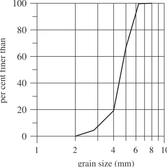
Figure 1. The grain-size distribution in the simulations is unimodal with a standard deviation of grain diameters of 1.33, range between 2 and 8 mm andd50= 4 mm.

A discrete particle model is presented here which simulates the transport of sed-iment as bedload in a unidirectional flow by applying simple physical rules to large numbers of spheres which represent discrete sediment grains moving within a flow. An equation of motion for sediment grains, collisions between grains, grain-flow momen-tum exchange and flow exposure are all accounted for in the model. The model is capable of tracking a large number of grains and is able to report the details of their individual movement, providing a degree of resolution which is difficult to obtain with current measurement techniques. The current model extends the earlier work on entrainment from uniformly sized sediments (McEwan & Heald 2001) to exam-ine the full-transport case including grain excursions and deposition. The aims of this paper are twofold. First, to present the model and demonstrate its success in reproducing some well-known features of sediment transport systems. Second, to demonstrate that key features of a sediment transport system can be reasonably well captured by a synthesis of four sub-processes: grain deposition, entrainment and saltation and a fluid feedback mechanism.

2. Modelled environment

(a) Initial conditions

(a₎ (b)

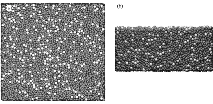
Figure 2. Plan and side view of the 200×200×80 mm sediment bed section simulated (50 000 grains).

larger bedforms do not form. Both lower stage and upper stage plane bed conditions are simulated.

Initial beds are formed by releasing a series of grains from random positions over a horizontal plane (z = 0) which defines the lower boundary of the bed. The grains accelerate under gravity and drop until at least half their volume is below the hor-izontal plane. Since the grains’ initial positions are random, the first grains to be released form an irregular foundation layer on which subsequent grains rebound into stable positions and are deposited to create a depth of sediment bed which is at least ten diameters of the largest grain in the simulated mixture (figure 2). Once deposited, the sediment bed is stored so that many simulations may use the same initial conditions.

The ‘sediment bed surface’ is defined as those grains that are not being rested upon by other grains. The sediment bed discussed in this paper consisted of 50 000 grains and was settled within still water.

It may be useful to the reader to have an estimate of the length of time taken to simulate sediment transport experiments. A 1 GHz Pentium III simulating 200 s of sediment transport of the mixture in figure 1 takes between 40 min and 3 days for mean bed shear stresses from 1 to 40 Pa. The rate of simulation depends upon the number of grains in simultaneous transport because over 50% of the model’s runtime is used to detect collisions between grains. To optimize the efficiency of the collision detection algorithm the model’s volume is divided into a mesh, each cube of which contains a list of references to any grains which intersect their volume. This ensures that the minimum number of neighbouring grains are checked for collisions at a minimal cost in terms of memory (ca. 200 Mb for the above simulations of 50 000 grains).

The dimensions of the settled bed are set by specifying the width and length of the model domain and the number of particles to deposit. The sediment beds pre-sented in this paper are large in terms of DPM (200×200×80 mm3

entrainment particle trajectory

calculation transport flow

deposition bed/inter-ballistic

collisions

flow velocity

momentum

initial position

rebounds

output

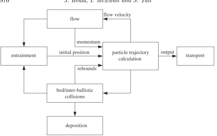
Figure 3. A simplified model flow chart demonstrating the connectivity of the main sediment transport sub-processes.

are of a similar order. The effective length of the sediment bed is therefore extended by applying periodic boundaries such that grains at one extremity of the bed sup-port grains on the opposite edge and saltating grains leaving one side of the model domain re-enter on the opposite side. The restricted size of the model domain and the operation of periodic boundaries make it necessary that only flat-bed equilib-rium transport is considered in this paper. The formation of ripples and other larger bedforms at scales comparable with the model domain would be undesirable, as the periodic boundaries would provide an unnatural constraint to bedform growth leading to their self-interference. Thus, the simulations presented here are restricted to lower and higher stage plane-bed conditions, omitting the intermediate range of shear stresses in which bedforms may dominate transport.

(b) Self-regulation of the transport system

During a sediment transport simulation there is a complicated exchange of momen-tum, such that each of the main physical sub-processes are interdependent and, through feedback, determine their own future operating conditions. For example, an entrained grain exchanges momentum with the fluid in the saltation layer and mod-ifies the fluid’s average velocity, which, in turn, determines the momentum available to entrain further grains. Figure 3 is a simplified flow chart demonstrating the inter-actions between the sediment transport and flow modification sub-processes, which are discussed in the following sections.

(c) Equation of motion and grain collision

equation for grain motion is therefore

ρs ρf

+ 0.5

dui dt =

ρs ρf

−1

gi+

3

4Ef

Cd(Re)

d |ui|(ui), where i= 1,2,3, (2.1)

where

Ef= grain exposure (between 0.0 and 1.0),

Cd(Re) = Stokes drag as a function of grain Reynolds number, gi=ith component of gravitational acceleration,

ui=ith component of grain velocity relative to fluid velocity,

d= grain diameter,

ρs, ρf= sediment and fluid densities.

Three-dimensional collisions between grains A and B result in a loss of momentum for each grain through the scaling of their velocity components normal to the impact plane by a coefficient of restitution of momentum, Rm. The grain velocities after

rebound are calculated using the following set of equations,

uAi=uA·ˆb, uBi =uB·ˆb,

uAf =

mAuAi−mBuAi+ 2mBuBi mA+mB

, uBf=

mBuBi−mAuBi+ 2mAuAi mA+mB

,

uA∆=RmuAf−uAi, uB∆ =RmuBf−uBi,

vA =uA+uA∆ˆb, vB=uB+uB∆ˆb,

⎫ ⎪ ⎪ ⎪ ⎪ ⎪ ⎪ ⎬ ⎪ ⎪ ⎪ ⎪ ⎪ ⎪ ⎭ (2.2) where ˆ

b= unit vector in direction normal to impact plane, uA, uB= velocities of grains A and B before impact,

uAi, uBi= velocities of grains A and B normal to impact plane,

uAf, uBf= impact plane normal velocities of grains after elastic impact, uA∆, uB∆= change in grain velocities considering coefficient of restitution

of momentum, Rm,

vA, vB= resultant velocities of grains A and B after collision.

However, if grain A has collided with grain B, which is static on the bed surface, it is assumed that the momentum transferred from A to B is dissipated through its contacts into the sediment bed. This special case is calculated by assuming mB is

very large (representing the mass of the sediment bed). SinceuBi= 0, equations (2.2)

reduce to

uAf→ −uAi, uBf→0, uA∆→RmuAf−uAi, uB∆→0.

(2.3)

0 t fluid shear stress h

h

s

bed surface

height

t

0

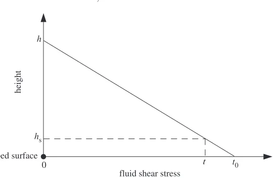
Figure 4. The streamwise shear stress profile of a flow over a sediment bed indicating the shear stress (τ) at the top of the saltation layer. The linear stress profile is a characteristic of two-dimensional open channel uniform flow in which the gravitational forces throughout the depth of the flow are balanced by fluid shear forces.

would, in reality, be substantially influenced, and probably dominated, by the irregu-larities of the sediment particles. Such algorithmic detail in a treatment of spherical particles is probably not warranted and if done inadequately would even mislead. By necessity, discrete particle simulations involve choices and compromise between increasing the detailed realism of the particle behaviour and increasing the model domain size and the number of particles. The model domain size, number of parti-cles simulated and the complexity of the algorithms have been adjusted in order to capture the essential physics of the problem while enabling simulations which track enough grains to reproduce the macroscopic or the emergent behaviour of the whole transport system.

(d) Momentum exchange between the flow and grains

Bedload transport is often constrained to a shallow layer over the bed surface such that the depth of flow h is much greater than the depth of the flow occupied by saltating grainshs (figure 4). Therefore, the mean fluid shear stressτ at the top of

the saltation layer is well approximated byτ0=ρghS.

Because the saltation layer is assumed to be thin, possibly only a few grain diam-eters in depth, velocity gradients are neglected and a uniform mean flow velocity is assumed to persist throughout the layer. As discussed in the next section, the mean flow impinging upon every grain is modified to represent spatial non-uniformities due to the sheltering effects of upstream grains. It would be unreasonable to define the bottom and top of the saltation layer to cover the range of heights over which grains experience drag forces since its thickness would depend upon individual grain positions (i.e. the highest and lowest unsheltered grains). Instead, the thickness of the saltation layer hs is calculated from the cumulative distribution of drag forces

0 20 40 60 80 100

95% of total drag force

5% of total drag force

height above bottom of bed (mm)

normalized cumulative drag force

0 0.2 0.4 0.6 0.8 1.0

thickness of saltation layer h

s

Figure 5. The saltation layer thickness is set by the 5% and 95% levels of cumulative drag force applied to the simulated grains.

The fluid shear stress applied to the saltation layer (τ0) generates a streamwise

body force at the centre of the layer. Thus, the total acceleration per unit area of the saltation layer is

ρfhsaf=τ0−

n

i=1

Fdi, (2.4)

where

ρf= fluid density,

hs= thickness of saltation layer,

af= acceleration of fluid in the saltating layer,

n= the total number of grains contributing to fluid drag per unit plan area, Fdi = fluid drag force onith grain, which includes both static and mobile particles.

0 400 800 1200 1600

0 0.4 0.8 1.2 1.6 2.0

saltation layer velocity (mm

s

−

1)

time (s)

0 5 10 15 20 25

sediment transport rate (kg

m

−

1s

−

1)

saltation layer fluid velocity (mms−1) 0 400 800 1200 1600

(a_{) (}b₎

Figure 6. The momentum exchange between saltating grains and the modelled fluid flow brings the fluid velocity and sediment transport rate quickly into equilibrium.

0 0.1 0.2 0.3 0.4

rate of change of momentum (kg m

s

−

2)

time (s)

0 2 4 6 8

Figure 7. A comparison of the total momentum supplied to the grains from the fluid (dark grey line) and that lost through grain collisions (light grey line).

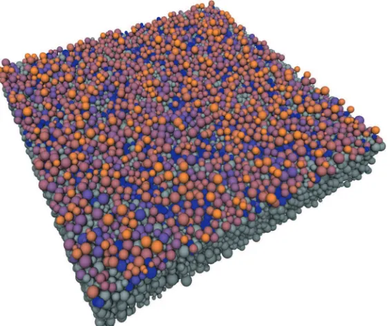
(e) Grain sheltering and exposure to the flow

The main forces producing sediment transport are the downstream horizontal drag forces on the grains from the mean flow. However, at the surface of a sediment bed, one particle is liable to be caught in the wake of another, and the mean horizontal flow velocity incident upon it is therefore reduced.

Figure 8. A sediment bed in which the grains are coloured according to their level of exposure.

their effects are compounded so that ifEfi represents the scaling of exposure due to graini at pointp in the flow, then the actual exposure,Ef, atp may be calculated

as the product of the exposure scaling from all the disturbances of local upstream grains,

Ef(p) =

i

Efi(p). (2.5)

The cumulative effect of flow reduction produces patches of bed surface that are partially exposed, grains saltating above the bed surface that are completely exposed, and grains deep within the sediment bed that are almost fully sheltered. Figure 8 is a graphical representation of the amount of exposure experienced by the bed grains (grey grains have no exposure, the colour shading from blue to orange as grains become more exposed). It should be noted that every grain reduces the flow downstream dynamically so that when it moves its effects on the flow are removed and reapplied at the new position, ensuring a high resolution of sheltering effects both temporally and spatially.

(f) Grain saltation

10 20 30 40 0

1000 2000 3000 4000

distance (mm)

time (s) 0

Figure 9. The time-series of travel distance of a 4 mm sediment grain saltating in a 900 mm s−1 _flow.

These initial rebounds are very small (ca. 10−8

mm) and, when animated, appear as a rolling motion. The authors suggest that the definition of rolling when applied to grains should be more carefully stated than it is currently in the literature. We would suggest that a perception of rolling results from a large number of small rebounds as the crystalline facets of two grains glance against each other.

Once a grain is entrained, its motion is governed by an equation of motion (2.1) and by collisions with other bed surface grains. These collisions convert stream-wise momentum into vertical momentum, thereby forcing the grain upwards into the flow, where it replenishes lost momentum before coming back into contact with the bed surface. If a grain lacks sufficient vertical momentum to saltate over the local bed surface then it rebounds repeatedly from the same set of static grains. This grain’s location is then taken as its position of deposition and defines the endpoint of its saltation excursion. As soon as a grain has been deposited, it is immediately available for re-entrainment, pending a change in the local flow conditions or a sufficiently energetic collision from a saltating grain.

The displacement over time of a single 4 mm grain over a mixed-sized sediment (as in figure 1) in a fluid flow velocity of 800 mm s−1

is plotted in figure 9. The grain’s saltation velocity is ca. 420 mm s−1

. Note that the history of its displacement has some important similarities to that proposed by Einstein (1950) in that it travels for short lengths of time between relatively long rest periods.

3. Results and validation

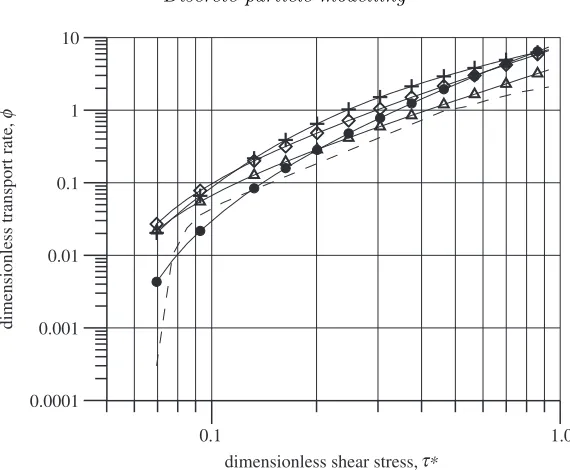
0.0001 0.001 0.01 0.1 1 10

dimensionless transport rate,

φ

dimensionless shear stress,τ∗

0.1 1.0

Figure 10. A comparison of bedload simulated transport with previous models: filled circle, Yalin (1972); triangle, Bagnold (1956); diamond, Meyer-Peter & M¨uller (1948); cross, Einstein (1950); dashed line, DPM.

Firstly, they have a steep increase in bedload transport at low shear stresses and, secondly, at high shear stresses they are asymptotic to a power law in which bedload transport is proportional to (τ0−τ0c)

n

, where n is either 1.0 or 1.5 andτ0c is the

critical mean bed shear stress for the initiation of bedload transport.

A set of simulations at increasing mean bed shear stresses was conducted with the model’s parameters set to arbitrary, yet realistic values: a coefficient of restitution of momentum Rm of 0.5 and a fluid sheltering distance of 8 grain diameters. The

results have been plotted in figure 10 as dimensionless bedload transport φ against dimensionless shear stressτ_∗ (usingd50 as the representative grain diameter):

φ= ρ

0.5

f gqs

((ρs−ρf)gd50)1.5

and τ_∗= τ0 (ρs−ρf)gd50

. (3.1)

The simulation results compare well with the traditional transport rate curves of Meyer-Peter & M¨uller (1948), Einstein (1950), Bagnold (1956) and Yalin (1972). Sediment grains begin to move at τ_∗ ∼ 0.07, which is very slightly higher than the often quoted values of the shields parameter used to categorize incipient motion. Furthermore, there is a marked change in transport regime at τ_∗ ∼ 0.1 and the transport rate curve becomes asymptotic to the lineqs∼τ1

.15

∗ at high shear stresses.

trans-dimensionless transport rate,

φ

dimensionless shear stress, τ 1 × 100

1 × 10−1

1 × 10−2

1 × 10−3

1 × 10−4

0.06 0.08 0.10 0.20 0.40

Figure 11. Bedload transport rate sensitivity to the coefficient of restitution of momentum. Black line,Rm= 0.3; grey line,Rm= 0.5; dashed line,Rm= 0.7.

dimensionless transport rate,

φ

dimensionless shear stress, τ 1 × 100

1 × 10−1

1 × 10−2

1 × 10−3

0.06 0.08 0.10 0.20 0.40

Figure 12. Bedload transport rate sensitivity to changes in the sheltering distance used in the DPM simulations. Black line, shelter = 4d; grey line, shelter = 8d; dashed line, shelter = 16d.

port rate with increasing mean bed shear stress for three different coefficients of restitution of momentum: 0.2, 0.5 and 0.7. Bedload transport rate sensitivity to a coefficient of restitution reduces as mean bed shear stress increases. Grains trans-ported in low shear stress simulations appear to remain close to the bed surface, undergoing frequent rebounds during which they lose streamwise momentum. At higher shear stresses the grains rebound higher above the bed’s surface and collide less frequently. Thus, their transport rates seem to be less sensitive to a coefficient of restitution.

As figure 12 shows, the changes in transport rate curves with sheltering distance set to 4, 8 and 16 diameters are relatively small.

4. Discussion

Two levels of model validation are available. We term these level 1 validation, in which the average or integrated model behaviour is compared with known data (e.g. mass-transport rates), and level 2 validation, which occurs at the detail of the constituent sub-processes and requires data from observation of individual grains’ behaviour. Data for level 2 are generally scarce compared with level 1 due to the difficulty of obtaining them. At level 2, verification of the model’s algorithms can be done by examining conservation of momentum and mass within the model domain and also, somewhat more subjectively, through consideration of the physical plau-sibility of the model behaviour. Visual observation of animations is in fact a pow-erful tool and has provided a useful contribution to level 2 validation. The human eye, trained in observing the detail of the physical processes, can detect algorithmic problems and issues in a way which lends some limited support to these other more rigorous validation methods.

Set against this is the recognition that the realism of the model is severely lim-ited in certain aspects of the small-scale processes. These limitations arise because of the compromises made between increased algorithmic complexity and the large number of discrete particles modelled. There are three of these which stand out as being particularly important. First, the treatment of particle wakes is, by necessity, simplistic. Second, the particles are treated as smooth spherical particles to maintain the tractability of treating large numbers of grains. Therefore, shape effects, which inevitably must be significant, are not considered here. Third, the treatment of inter-particle collisions is idealistic in that the coefficient of restitution of momentum is used to account for frictional losses (Nino & Garc´ıa 1994), as well as grain shape and the expulsion of fluid from between the colliding bodies. It is extremely difficult to account for any of these processes faithfully.

The discrete particle model treats the transport process as a whole at an unprece-dented level of detail but, at a certain point, all models are an abstraction of the real process in observation. The aim of a simulation is to incorporate all of the key physical processes sufficiently well so that the original system is replicated. We can judge the completeness of the model by noting that, despite the gross simplifica-tions mentioned above, it produces data that validate successfully at level 1. Thus, future investigation of the parallels between the model’s micromechanics and real observations is essential so that its level 2 behaviour can be assessed.

5. Conclusions

(i) The model successfully reproduces significant macroscopic details of the trans-port system.

(iii) The model contains two ‘free’ physical parameters, namely, coefficient of resti-tution and sheltering length. Sensitivity analysis demonstrates that

(a) the sediment transport behaviour near threshold is very sensitive to the coefficient of restitution but above threshold the deviation in bedload transport rate with Rm becomes less significant; and

(b) the sediment transport rate becomes insensitive to the sheltering length at values less than 8 grain diameters.

(iv) The model is not able to simulate ripples or bedforms in a satisfying manner due to limitations in the size of the modelled domain and the increased complexity of the flow around bedforms. Therefore, simulations have been restricted to plane bed conditions.

(v) A realistic reproduction of the bedload transport system, which manifests a number of its key macroscopic features, has been achieved by creating an ideal-ized model consisting of only fluid drag, grain–grain and grain–fluid momentum exchange and bed surface sheltering.

References

Bagnold, R. A. 1956 The flow of cohesionless grains in fluids.Phil. Trans. R. Soc. Lond.A249_,

291–293.

Cundall, P. A. & Strack, O. D. L. 1979 A discrete numerical model for granular assemblies. G´eotechnique 29_{, 47–65.}

Drake, T. G. & Calantoni, J. 2001 Discrete particle model for sheet flow sediment transport in the nearshore.J. Geophys. Res. Oceans 106_{(9), 19 859–19 868.}

Einstein, H. A. 1950 The bedload function for sediment transport in open channel flows. Tech-nical Bulletin 1026, Soil Conservation Service, US Department of Agriculture, Washington DC.

Francis, J. R. D. 1973 Experiments on the motion of solitary grains along the bed of a water stream.Proc. R. Soc. Lond.A332_{, 443–471.}

Gotoh, H. & Sakai, T. 1997 Numerical simulation of sheetflow as granular material.J. Wtrwy Port Coastal Ocean Engng 123_{(6), 329–336.}

Haff, P. K. & Anderson, R. S. 1993 Grain scale simulations of loose sedimentary beds—the example of grain-bed impacts in aeolian saltation.Sedimentology 40_{(2), 175–198.}

McEwan, I. & Heald, J. 2001 Discrete particle modelling of entrainment from flat uniformly sized sediment beds.J. Hydraul. Engng ASCE 127_{(7), 588–597.}

Meyer-Peter, E. & M¨uller, R. 1948 Formulas for bedload transport.Proc. 2nd Congr. Interna-tional Association of Hydraulic Research, Stockholm, pp. 39–64.

Nino, Y. & Garc´ıa, M. 1994 Gravel saltation. 2. Modelling.Water Resources Res.30_{(6), 1915–}

1924.