Algorithms in time series

by

Andrew McDougall

A Thesis submitted to the

AUSTRALIAN NATIONAL UNIVERSITY

for the Degree of

DOCTOR OF PHILOSOPHY

I am indebted to my supervisors, Professor E.J. Hannan and Dr. D.S. Poskitt, for their invaluable assistance and encouragement throughout my stay at ANU. I would like to give special thanks to Ms. D. Cook for the superb graphics and finally, I would like to thank my parents for all their support.

The use of finitely parametrized linear models such as ARMA models in analysing time series data has been extensively studied and in recent years there has been an increasing emphasis on the development of fast regression—based algorithms for the problem of model identification. In this thesis we investigate the statistical properties of pseudo—linear regression algorithms in the context of off-line and online (real-time) identification. A review of these procedures is presented in Part I in relation to the problem of identifying an appropriate ARMA model from observed time series data. Thus, criteria introduced by Akaike and Rissanen are important here to ensure a model of sufficient complexity is selected, based on the data.

In chapter 1 we survey published results pertaining to the statistical properties of identification procedures in the off-line context and show there are important differences as concerns the asymptotic performance of certain parameter estimation algorithms. However, to effect the identification process in real-tim e recursive estimation algorithms are required. Furthermore, these procedures need to be adaptive to be applicable in practice. This is discussed in chapter 2. Technical results and limit theorems required for the theoretical analysis conducted in Part II are collated in chapter 3.

Chapters 4 and 5 of Part II are therefore devoted to the detailed investigation of particular algorithms discussed in Part I. Chapter 4 deals with off-line parameter estimation algorithms and in chapter 5, the important idea of a Description Length

Principle introduced by Rissanen, is examined in the context of the recursive estimation of autoregressions. Empirical evidence from simulation experiments are also reported in each chapter and in chapter 5, aspects of speech analysis are incorporated in the simulation study. The simulation results bear out the theory and

Declaration (i)

Acknowledgements (ii)

Summary (Hi)

Contents (iv)

Introduction (vi)

Notation (ix)

PART I : PROCEDURES

Chapter 1: Estimation of ARMA Models

1.1 ARMA Models 1

1.2 Identification 4

1.3 Maximum Likelihood Estimation 10

1.4 Pseudo—Linear Regression 17

1.5 Order Selection 26

Chapter 2: Recursive Estimation

2.1 Introduction 36

2.2 Recursive Least Squares 38

2.3 Adaptive Estimation 46

2.4 Recursive PLR Algorithms 52

2.5 Recursive Order Selection 56

Chapter 3: Theoretical Analysis

3.1 Prelude to Part II 63

3.2 Preliminary Results and Conditions 64

3.3 Autoregressive Approximations 67

3.4 Toeplitz Calculations and ARMA Estimation 71

3.5 Some Matrix Theory 75

PART I I : APPLICATIONS

Chapter 4: Regression Procedures

4.1 Chapter Outline 79

4.2 Algorithms 80

4.3 Modifications 85

4.4 Simulations 87

4.5 Theoretical Analysis 97

4.5.1 SPL 99

4.5.2 LRR 108

4.5.3 HR 115

Chapter 5: Recursive Estimation of Autoregressions

5.1 Introduction 122

5.2 Rissanen's Principle and SPR 124

5.3 Simulations 128

Appendix 5. Proof of Theorem 5.2.1 142

Models are fundamental in science and come from past experience and from

theory. They provide an aid to understanding the properties of a system (whose behaviour we may be interested in analysing, affecting or controlling), and underlie solutions to problems. In time series, the exact structure of the mechanism generating the process is usually unknown and one is naturally led to consider the observed signal as a realization of a stochastic process. The problem of model identification from measured data has been extensively studied and in particular, the estimation of parameters within models. An important part of this problem is recursive identification and the associated parameter estimation algorithms.

In this thesis we consider the statistical properties of algorithms associated with the identification and estimation of finitely parametrized ARMA models. These models, made popular by Box and Jenkins (1970) in their influential book, are widely used in statistics, systems engineering and econometrics to describe stationary processes. In practice, the data may exhibit charactistics suggesting non—stationarity (eg. seasonal or trend components), in which case the time series needs to be transformed so as to achieve stationarity. Common transformations are differencing, Box and Jenkins (1970), and trend—regression, see Anderson (1971), Hannan (1970). However, we shall not be concerned with these matters and assume that this model class is appropriate for modelling the (possibly transformed) time series.

Identifying a particular ARMA model involves the selection of order which in turn, corresponds to the number of parameters that need to be estimated. Thus, we

models of different orders. These criteria use the data to determine the order rather than a priori knowledge, and under the assumption that a true model exists (and is

contained in the model class considered), certain consistency results can be established. Furthermore, using these criteria the order selection process can be systematized to a large extent through repeated use of a suitable parameter estimation algorithm.

The choice of algorithm depends on the application and, in practice, an algorithm would be implemented in a form modified to cater for specific requirements. However, an important factor in any application is whether the identification process is required online, that is, during the operation of the system,

for example, to allow decisions to be made according to the current state of the system. In this situation, it is necessary to identify the models at the same time as the data is collected. The model is then "updated" as new data becomes available and the updating can be performed by a recursive algorithm. This is referred to as recursive estimation. Of course, off-line procedures, which are based on all the data, could be used to perform the updating and may be more appropriate if the data is collected in "batches". Hence, off-line identification is also called batch

identification. However, because an upper bound can be put on the number of calculations required for recursive estimation at each update, recursive algorithms can be effected in real-time where a fixed time interval exists between successive observations. Thus, we use the term recursive identification for procedures that can be implemented in this context.

we do not discuss algorithms as they might be realized as computer programs. Indeed only the general form is required, wherein design variables may need to be

specified by the user. The effect that these choices have on the properties of the parameter estimates is investigated analytically. Conducting the analysis in conjunction with simulation studies provides a useful guide to the applicability of an algorithm.

However, the analytical treatment involves extensive calculations, thus for

clarity, the thesis is presented in two parts. In Part I a range of procedures and techniques used for the identification of ARM A models are presented. In chapter 1, after formally defining the ARMA model and the associated identification problem, estimation methods are dealt with in the off-line context. Recursive algorithms are examined in chapter 2. As mentioned above, these algorithms can be computed in real-tim e and the implementation of a recursive order selection strategy is also discussed. The techniques and conditions required for the analytic treatment of the algorithms that we investigate in Part II is given in chapter 3, which concludes Part I. Thus, Part II contains the results obtained from statistical analyses and simulation studies of particular algorithms that have been discussed in Part I. Chapter 4 examines off-line regression procedures for parameter estimation where the order of the ARMA model is assumed to be known. The recursive estimation of order in relation to autoregressive processes is considered in chapter 5. In Part II the

Abbreviations

A M L a p p r o x im a te m a x im u m lik elih o o d

A R a u to re g re s siv e

A R M A a u to re g re s siv e m o v in g a v e ra g e

a.s. a lm o s t su re ly (w ith p r o b a b ility 1)

C L T c e n tra l lim it th e o re m

EL S e x te n d e d le a s t sq u a re s

H R a lg o rith m (A l.4 .3 )

L R R a lg o rith m ( A l.4 .2 )

L S E le a st sq u a re s e s tim a te

M A m o v in g a v e ra g e

M D L m in im u m d e s c rip tio n le n g th p rin c ip le

M L E m a x im u m lik elih o o d e s tim a te

P M D L p re d ic tiv e m in im u m d e s c rip tio n le n g th p rin c ip le

P L R p se u d o —lin e a r reg ressio n

P R C p o s itiv e re a l c o n d itio n

R LS re c u rs iv e le a st sq u a re s

R M L re c u rs iv e m a x im u m lik elih o o d

S P L a lg o rith m ( A l.4 .1 )

Symbols

A N a s y m p to tic n o rm a l d is tr ib u tio n

r

re a l p a r t of c o m p le x v a ria b le z

«y

A®B te n s o r p r o d u c t of m a tric e s

a(z) AR 2:—transform

b(z) MA 2—transform

k(z) rational transfer function

T sample length

q t (io g io g r/T )l/2

h t

(logT)a, a < oo

0 unknown parameter vector

00 true value

On off-line estimate at nth iterate

0(t) recursive estimate

y(t) observed data

f ( < ) white noise sequence

f ( < ) residual estimate

i ( t , 0 ) residual estimate using fixed 0 a—algebra generated by e(s), s <t Xk{t) regressor variable of dimension h

Ch (t) prediction error from a model of dimension h

4

A forgetting factor

At(«) forgetting profile

Estimation of ARMA Models

§1.1 ARMA Models

Linear systems are widely used to describe the behaviour of physical processes because, notwithstanding their structural simplicity, experience shows that they work well. For stationary stochastic processes autoregressive moving—average (known as ARMA) systems play an important role in modelling time series. In the remainder of this section we define the ARMA system, introduce some of the associated terminology and briefly discuss conditions relating to the uniqueness and stability of such a system.

Let y(t) be a discrete-time, stochastic process satisfying an equation of the form

(i-i.i)

J 0«ü

) y { t - j )

- ft(o)=/?(o)=i

Then y(t) is said to be an ARMA(p,q) process where the order parameters p,q refer to the highest lags in (1.1.1). If y(t) consists of m components then (1.1.1) describes

a vector ARMA process where the a(j),/?(j) are ra*m matrices and a(0)=/?(0). (But not necessarily o(0)=Im). The addition of an observed input or exogenous variable

u(t) can also be included whereby (1.1.1) is known as an ARM AX process, the X referring to the presence of an additional input. The sequence y(t) is often called the output or endogenous variable and it is assumed that the sequence of unobserved

inputs, e(£), are stationary and ergodic and satisfy

(1.1.2) £[e{t)\ = 0 , = <72£st

In the vector case, o2 is a positive definite matrix. However, we will only be dealing

with the scalar ARMA case, m = l, hence shall not be further concerned with details relating to vector models or additional inputs. The assumption £[e(£)]=0 means that, in practice, the data will need to be mean—corrected but since this will not

make any difference to the asymptotic results we obtain later, we ignore it for

simplicity.

The functions

(1.1.3) a(z) = S Qa ( j ) z j , b(z) = S (^ ( j ) z J,

are called the generating polynomials or z-transforms for the process (1.1.1) and

treating 2) as a lag operator (i.e. zy(t)=y(t-1)) we can write (1.1.1) as

(1.1.4) a(z)y(t) = b{z)e{t)

The ^-transforms, a(z),b(z) are assumed to be coprime (i.e. have no common factors) and have no zeros on or inside the unit circle:

(1.1.5) a(z),b(z) / 0 , I z\ <1

As a result of (1.1.5) the e(t) are then also the linear innovations. That is, e ( t ) = y ( t ) - y ( t \ t- l ) where y ( t \ t - l ) is the best linear predictor (in the least squares sense) of y(t) from y(s), s<t. Note that y ( t \ t - l ) is a theoretical quantity and like e(£), is not observable. These statements also have vector analogues and, as with any of the results asserted here, are established in Hannan (1970) and Rozanov (1967). For the asymptotic analysis it will be necessary to further restrict e(t) and for our purposes the following conditions will suffice.

(1.1.6) £[c(t) |J t-i]=0, £[c(t)2\7t-\\=(r2, £[e(t)A}<oo

is the a—algebra of events determined by e(s), s<t. These conditions will be discussed again in chapter 3, however, the first part of (1.1.6) means that the e(t) are martingale differences. (Note that it is also equivalent to the statement that the best linear predictor is the best predictor).

When (1.1.5) holds, (1.1.4) can be written as

00

(1.1.7) y(t) = k(z)e{t) , W = J 0* 0 ) A *(°)=1

(1.1.8) J 0«(j)2 < oo

If e(t) is to be the innovation sequence for y(t) we require, (1.1.9) k(z) ± 0 , I z\ < 1

Now if (1.1.7),(1.1.8),(1.1.9) hold with k(z) rational so that k(z)=a(z)~1b(z) where

a(z),b(z) are polynomials, then (1.1.1) also holds. Note that (1.1.9) shows that a stationary solution of (1.1.1) is still possible when b(z) has zeros on |2 |= 1 . However we need to exclude this possibility and this is reflected in (1.1.5).

So far, the above assumptions have been made in order that theoretical results may be established, however, there are also important numerical consequences, particularly when the boundary conditions are approached. For example, should b(z) have a zero near \ z\ = l or there be near common factors, numerical instability in the estimation procedure may result. Both these situations constitute "critical cases" and play an important role in the simulation studies carried out in chapter 4.

We can also characterize the structure of a stationary process such as (1.1.1) through the autocovariance sequence

(1.1.10) 7 (r) = S[y{t)y(t+r)]

The autocorrelation function is defined by p{r)=°f(r)/1(0). From (1.1.7),(1.1.2) it can be seen that

00

(1.1.11) 7(r) = KCf*-r) , r> 0 = 7(r)

If g(cj) is the function with Fourier coefficients 7(r) then the spectral density, g(u), has the Fourier series

00 2

(1.1.12) 2 i ^ 70)e“ ’;u' = I*(«'")I2 > we[-jr,jr]

(Writing kk?=\k\2 since it is a scalar variable, * denoting conjugation with transposition). The spectral density g((j), has direct a physical meaning in terms of

the Fast Fourier Algorithm, it may in fact be more efficient to carry out computations in the frequency domain even when the time domain approach is adopted. However, the mathematical equivalence between the frequency domain and time domain means that it is only a question of representational value. In the analytic treatment it will be convenient to use a spectral representation of certain quantities. For example,

(1.1.13) 7( j ) =

f

The representation (1.1.12) is also unique subject to (1.1.9) and <j2>0. Thus,

given a complete realization k, a 2 can be uniquely determined. Of course, we only ever see part of a realization hence the statistical problem of estimating these parameters. Since we can regard (1.1.1) as an approximation to (1.1.7), this corresponds to the problem of identifying the parameters in a model of the form (1.1.1). This is now discussed.

§1.2 Identification

The identification of an appropriate ARMA(p,</) model to represent an observed stationary time series involves a number of inter—related problems. These include the choice of p and q (order selection), and the subsequent estimation of the parameters a (j)j= l,...,p , and innovation variance a2. In addition to the standard assumptions given in section 1.1, namely (1.1.2),(1.1.5),we assume there are no further restrictions on the a(j),/?(j), (or a 2). In selecting the order we shall use information criteria of the type introduced by Akaike (1974) and Rissanen (1983) which are discussed in section 1.5 along with other methods. Thus, the

structure of the model we fit to an observed sequence of length T say, which we denote by y = ( y ( l),...,?/(T))', is determined by the data rather than a priori knowledge.

in the sequence yT are assumed to be available before any modelling procedure is effected. Thus, implicitly, y represents a "batch" of data of fixed length T, which

has been stored as it was collected. Hence the alternative terminology. Clearly then, it is only the order of the observations in y and not the actual time of recording, which is of consequence. Because y has been stored, several ARMA models can be

examined and compared by reprocessing the data. The comparison of different models can be systematized to a large extent by using some type of information criterion to select an appropriate order. Here we choose h=p+q to minimize a function of the form

(1.2.1) log bl + hC{ T) / T, h < H

where H may depend on T, C( T) is a prescribed sequence and is an estimate of a2 assuming the order to be h. Because (1.2.1) and order selection methods in general, are calculated by the repeated application of parameter estimation algorithms over a specified range 0<h<H, we have left a detailed discussion of order selection procedures and their properties until later in section 1.5. Hence, we shall assume for the present, that this part of the identification procedure has been carried out. It remains to consider the problem of estimating the parameters of a particular model, for given p, q. The advantage of working in the off-line context, is that the data can be processed all at once and more importantly, since the data can be reprocessed, the parameters can be re—estimated using possibly a different algorithm, to obtain better estimates. As we shall see, a modelling strategy

incorporating (1.2.1) can be employed to significantly reduce the computational cost involved in obtaining good parameter estimates. Although in some cases it may not be practical to process the data all at once, (e.g. a large amount of data), we assume the estimation procedures used in off-line identification can be considered to have

processed the data in this manner.

future action can be made based on the current state of the system. Then these decisions can be updated as new information is received. For example, in electricity load forecasting, ARMA models can be used to provide regularly updated, short-term predictions of the future power demand. (See Frick and Grant, 1985, Abu—el—Magol and Sinha, 1982). Decisions based on these predictions therefore lead to the more efficient production of electricity. In this type of situation, the use of off-line procedures to perform the model updating from y1 to yul at each t, may be prohibitive in terms of the increasing number of calculations required since all the observations in yui will be used. In fact, it becomes impossible if the sampling frequency, 1 /At, where A t is the real-tim e interval between observations, is high, as is the case in speech encoding, for example. In the next chapter we investigate recursive identification procedures which solve this problem. Thus, for the remainder of this chapter off-line identification is considered.

To compare the performance of different estimation procedures the statistical properties of the estimates are investigated. Under the assumption that a true model of the form (1.1.1) exists, consistency results can be established. We shall always distinguish the true model by a zero subscript as in (1.2.2)

v o ?o

(1-2-2) 2 0ao{j)y{t-j) = Zo0o(j)e(t -j) ,a o(0) = /?o(0) = 1

£[e(i)]=0 , f [ e ( l ) e ( s ) ' ] = 4 t

The generating polynomials a0(z), b0(z) are equivalently defined as in (1.1.3) and the standard assumptions of section 1.1 are assumed to hold for (1.2.2). Without

loss of generality we will also often take <Jo=l. For convenience, we introduce 9 as a general coefficient parameter vector, so that, for example, 90' = (a0(l),...,a0(p0), ß0(l),...,ßo(q0)). Hence (1.2.2) may be written as

(1-2.3) y(t) = Oo'xo(t) + e(t)

of 0 can be used for comparing the performance of different estimation procedures. Suppose qo= 0 so that (1.2.3) defines an autoregressive (AR) process of order p 0

v o

(1-2-4) Z 0« o ( j ) y ( t - j ) = e ( 0 Then (1.2.4) satisfies the Yule—Walker equations,

(1.2.5) r o 0 = o g = 7 ( 0 ) + V C

where T is the autocovariance matrix, [ y ( j - k

) ] ,

1,.. .p0J

, . . . ,

7(^0)). Here, 0o consists only of the a 0(j). Because of ergodicity and (1.1.2) we have that,

T - r

(1.2.6) c(r) = r 1 ^ y ( i ) y ( t + r ) —► 7(r) fl.s.

Hence asymptotically, a consistent estimator of 0o can be obtained by solving (1.2.5) with c(r) in place of 7(r). This is known as the Yule—Walker estimate which we denote as 0yw- Because of the Toeplitz structure of T, the matrix inversion required for the direct solution of ^yw can be avoided through the use of the fast Levinson—Durbin Algorithm given below.

A l.2.1 Levinson-D urbin Algorithm for AR Models

If c(0)>0, then the parameters 0m a l of an AR(ra) model, ra = l,2 ,...,T -l can be recursively calculated as,

m —1

( 1 . 2 . 7 ) 0n(m) = - j. S 0 0m-i(j) c(m-j)/ a\. 1 , ^ m ( 0 ) = 1 , V/n

K( j ) = t f m - i ( j ) + On(m)0m.i(m-j) , j = 1 , . . . , / w - l

c l = (I- ^m(/w)2)^m-l, ^m=0 = c(0).

Note that the öm(m)'s are estimates of the partial autocorrelations (also called reflection coefficients) and as a result of the last recursion in (1.2.7) this algorithm could also be used to estimate p 0 in (1.2.4) by the criterion given in (1.2.1).

However, for an ARMA process a linear relationship is not obtained. Indeed for

( J o - r

cl 2, ßo{j)ßo{j+r) , r = 0,1,...

(1.2.8) 7(r) = l

I 0 , r > q0

which is non—linear and would need to be iteratively solved. The determination of the ß0(j) from the 7(r) via (1.2.8), is spoken of as the spectral factorization since, from (1.1.12), we have

2 Qo

(1-2.9) X0ßoU)e'3U

(The property, (1.2.9), will be used later in chapter 4). In practice, a solution based on (1.2.8) using c(r), is not recommended since the estimates can be shown to be very inefficient. See, for example, Brockwell and Davis (1987, p246) where the

MA(1) case is discussed.

Alternatively, we can regard (1.2.4) as a straightforward regression where the regressor variable x(t) consists of lagged values of y(t) only. Hence, for (1.2.4) the Least Squares Estimate (LSE) for 0o, #Lg say, is given by,

A l.2 .2 Least Squares E stim a te -A R Model

(1.2.10) §LS = -P(T)n(T)

where

(1.2.11) P(T)-' = 1 ^ 1 ) ' , u(T) = l ^ t ) y ( t )

In (1.2.11), only positively indexed terms of y(t-j) are included in the sums of squares and cross products, so that p0- r estimates of 7(7*) will be formed in T XP{T)"1. Hence, P(T)'1 does not have a Toeplitz structure and the LS estimates are different to the Yule—Walker estimates for finite T. Asymptotically this difference becomes negligible and it can be shown that both estimates have the same limiting distribution (Hannan, 1970). Indeed in Part II, the assumption of a Toeplitz structure considerably simplifies the asymptotic analysis and we shall

However, there are some important differences for finite T. Let 0 (z), 0 J z )

I W L o

denote the z—transforms associated with the Yule—Walker and Least Squares estimates, respectively. That is,

v o A

0YW

(z) = 1 +

W

0V>

with 0 J z ) defined in similar fashion. The advantage of Yule—Walker estimates is that 0Yy{z) is guaranteed to be stable in the sense that 0 {z)^0, \z\<l, (Hannan, 1970), whereas 0 (2) is not. It is shown by Cybenko (1980) that the Levinson— Durbin Algorithm is also numerically stable (in terms and fixed or floating-point arithmetics) and comparable to the Cholesky algorithm which would typically be used to solve (1.2.10). Often, no stability problem arises and the stability can be

easily checked and rectified if necessary as we shall see in section 4.3. A disadvantage is that it is known 0yw can be severely biased in small samples and is in general inferior to LSE's (Tjostheim and Paulsen, 1983). The same bias effect also occurs when al is calculated from (1.2.7) (Paulsen and Tjostheim, 1985). As the bias inflates the value al this would affect the order estimates obtained from

(1.2.1).

One of the main reasons for examining AR estimation is that, under (1.1.5) we can write (1.2.2) as

(1.2.12) M z)y{t) = > <Po(z) = KizY^oiz)

which represents an AR(oo) process. Furthermore, as k(z)A exists from (1.1.7) then putting ip0(z)=k(z)A in (1.2.12) defines a more general model. Thus, approximating (1.2.12) by a finite AR process of order h say (by choosing h arbitrarily large or via (1.2.1)), means that a computationally inexpensive estimate, 6h, can be obtained. Of course, 6h cannot be a consistent estimator unless h is allowed to tend to infinity. However, often a good fit to the data can be obtained for moderate h and

consequently autoregressive approximations are widely used in practice.

detected due to the all—pole filter. (This is another term for the generator a(z)_1). It can be seen from (1.2.12) that if b0(z) has a zero near |z |= l , the coefficients of (p0(z) will only decrease slowly to zero and hence h may need to be large for a good approximation to be obtained. In this case, an ARMA model may provide an equally good, but far more parsimonious, fit to the data.

In the next section maximum likelihood estimation of ARMA processes is discussed which provides accurate, but computationally expensive parameter estimates. Therefore, an alternative procedure is presented in section 1.4. In both

cases off-line estimation is assumed where the orders p0,</o of the ARMA model are known or have been estimated. Again, we deal with that question in section 1.5.

§1.3 Maximum Likelihood Estimation

T

Suppose for the observation sequence y , we can associate a T-dimensional random variable whose known probability density ?(y ) depends on some unknown parameter, ip say. Then from the likelihood principle (assuming the model is correct), all the information that the data can provide about ip is contained in the likelihood function C*(ip\y ), which is of the same form as 7(y ) except that y is treated as fixed. This is therefore an appropriate function for estimating ip and the value of ip which maximises the likelihood function is called the maximum likelihood estimate (MLE). In our case, ip denotes the p+q+l parameters (0,cr2) of the ARMA model (1.1.1). Again, we are assuming the data is mean corrected. For the case of an ARMA model with nonzero mean, the reader is referred to Anderson (1971). It will

be more convenient to work with a log—likelihood function, - 2 T ' l\og[C¥(ip\ ?/T)], which on Gaussian assumptions and omitting constant terms is given by

(1.3.1) £(</>)= r 'l o g detGt(V>) + r 1yT'GT(V>)-1/

where G (ip)=£[y^y^']. Thus the MLE of is obtained by minimizing (1.3.1).

because we can regard (1.3.1) as a measure of the goodness of fit of the covariance matrix G (ip) to the data. Hence, choosing ip to minimize (1.3.1) is still sensible even if y is not Gaussian. Furthermore, the asymptotic properties of the resulting MLE can be established under much weaker conditions. (Such conditions will be discussed later in chapter 3).

Since a MLE is the best we can do (according to the likelihood principle), its

asymptotic properties provide a lower bound to which the properties of estimators obtained by alternative procedures can be compared. An estimator is said to be efficient if it has the same limiting distribution as that of an equivalent MLE constructed an Gaussian assumptions even though Gaussian assumptions are not maintained. Therefore, the performance of an identification procedure may be judged, in part, by the efficiency of its estimates. At the end of this section we shall state what the asymptotic properties of a MLE are, but it is of interest to examine how the optimization of (1.3.1) can be carried out.

In general, there is no explicit expression for the MLE and the optimizing value needs to be iteratively calculated. When explicit expressions for the elements of GT (ip) are used, the procedure is referred to as exact. (Since under Gaussian assumptions the resulting MLE would indeed be exact). However, these expressions are usually complicated functions of parameters in ip, and approximations are frequently made to reduce the amount of computation required for the optimization process. This is well illustrated even in the simple Gaussian AR(1) case.

MLE: AR(1) Case

Consider the AR(1) process

(1.3.2) y(t) = a y { t -1) + e(t) , | or| <1, e(t)~N(0,<72) To initiate the realisation ?/T, suppose y (0) is available. Then

£*(0I iT.j/(o)) = ;n 1 I yt_1,y(o))Ay{o))

M 2*

* (jr^2)"1/,2exp{ y(0)2( l - a 2) 2 ? (2/(< )-«K < -l));

Giving

(1.3.3) C(ip\ yT,y(0))= lo g r2 - ^ - l o g O - f t 2)

+ ^ T ^ K ° )

2

(

1

-

2)

Thus, the minimising value of a satisfies

(1.3.4) 7l + - J j K O K * - 1) = 0

Since 7i=cr2£ * /(l-a 2), algebraic expressions for the minimizing values of a, given a2, would be the solution of a cubic equation.

Clearly, for general AR(p) processes, the equations become more complicated. Now, if instead, we were to compute the likelihood using the conditional probability density ?(y \ y(0)), the minimizing values are readily obtained as

(1.3.5a) it = ^ y ( t - l )y(t)/t^ y { t - l

(1.3.5b) a2 = (y (t)-i* y (t-l))2

With ?/(0) included, these estimates are just the LSE's that would be obtained from (Al.2.2) in the previous section. This approximation leads in general, to the minimization of a sum of squares and may loosely be described as "least squares" estimates. (We shall return to this point later). However, it can be seen that the main difference between the respective a estimates is that the effect of the initial

value y(0), namely the presence of 71 in (1.3.4), is ignored when ?(y \ y(0)) is used. However, this effect becomes negliglible as t increases and it can be shown that the respective estimators have the same asymptotic properties.

Of course in practice, only y is available to estimate ip, so that the preperiod

choice of its unconditional expectation, which is zero. Similarly, for the general ARM A process we set the preperiod values, {y(t),e(t)}=0, t< 0. The assumption of zero inputs and observations before t=\ is referred to as prewindowing. Asymptotically this approximation makes no difference and since its effect is usually

negligible in most samples where T is sufficiently large, it is commonly used. Note however, this means the resulting MLE's are now conditional on this choice and for small samples this approximation can lead to poor estimates, particularly if b(z) has its zeros near |z |= l . (See Pagan and Nicholls, 1976). In that case, a transient effect

may be introduced if y( 1) is not close to zero which may take some time to die out. An example of this is given in Box and Jenkins (1970, p219).

To obtain unconditional MLE's of an ARMA process the exact likelihood function needs to be used which, in the form of (1.3.1), is given by

(1.3.6) C{9,<?) =

l o g - r'log

(1.3.7) _< to

X

>

8

1

II

S

T

S

T

II

S

'

and (1.3.8) where

* e ( 0 ' = ( —

i)»---»—

P)»ce(f —

«))

Here, we have adopted the notation of Box and Jenkins (1970, chapter 7) where details of the derivation of (1.3.6) may be found. (See also Newbold, 1974). Thus o■2Mt(0)~1=Gt(0) and [ee(£)]= £[e0(/) | yT,0\. Therefore, the residual sequence ee(£) defined by (1.3.8) represents an estimable function of the unobserved inputs, e(t). The subscript 9 has been added to emphasize that the relationship is not linear.

Note that [ce(^)]=€e(0?

^>0-For an AR(p) process however, S (0) can be obtained directly. Consider again

ST(a) =

I

” 00 ” 00

Now £ [ y ( t ) \ y T ,a\ = 1), t < 0, so that £[ca (t) \ yT ,a] = a t - \ l - o ? ) y ( l ) , t < 1. Therefore,

S ^ H l - ^ M l f + J ^ J / W - a ^ - l ))2

Note that with detM (a) = l - o 2, the minimizing value of a obtained here, satisfies exactly the same equation given by (1.3.4), but relative to the realization y only.

These results can be obtained by more direct methods as shown in Box and Jenkins (1970, Appendix A7.4) for the AR(p) process and Newbold (1974) for the general ARMA(p,</) process.

The difficulty that arises is that even when M^{6) is known, its elements are in general, complicated non-linear functions of the 0 components. However, the direct calculation of M (0) can be avoided by using an algorithm such as the Kalman Filter (Melard, 1984) or Innovations Algorithm, Brockwell and Davis (1987, Proposition 5.2.2), to effect a Gram—Schmidt orthogonalization of the y sequence. Thus, G (ip) and ce(J) are expressed in terms of one—step predictors y0(£ |£ -l) so that the function (1.3.6) to be minimized becomes

(1.3.9) L (0,<r2) = r 1

Jjlog

where ve(Q—><72. The advantage here is that (1.3.9) can be calculated recursively

and in the case of the Kalman Filter, the derivatives required for optimization can also be calculated recursively. Even so, the amount of computation required may still be considerable.

In many situations, exact maximum likelihood estimation is not required and a significant reduction in the amount of computation is possible by optimizing

(1.3.10) c{o,a2)=iog<r2+<r~2

r lsT(

Thus the M%(0) term in (1.3.6) is ignored. Indeed, it was pointed out by Whittle (1951) in a more general context, where y(t) is in transfer function form as in

W hittle likelihood and approximate ML procedures in the frequency domain which

have been investigated by Walker (1964), Hannan (1969) and more recently Godolphin (1984). (See also Hannan and Diestler (1988, chapter 6) for an informative discussion). Hence, for T sufficiently large, the estimates obtained from

(1.3.10) should be little different to those from (1.3.6) which is often the case. Note that (1.3.10) results from using the conditional probability distribution ?(y \ y )

(where y represents the preperiod values) to calculate the likelihood. Thus (1.3.10) is often called the conditional or marginal likelihood. (Levenbach, 1972, used the marginal likelihood of standardized residuals to compute AR estimates). For simplicity we shall assume the approximation y =0 is used, although the method of back forecasting (described in Box and Jenkins, 1970) could be used to estimate y .

Since the minimizing value of a2 for given 6 is a2 = (0), where now 5T= E ^_ 1ee(Q2, the optimization of (1.3.10) can be effected by minimizing the concentrated likelihood function

(1.3.11) Cc(0) = ST(0)

As the orders are assumed to be known here, Astrom and Söderström (1974) show that lim ^ ^ Cc(0) has a unique local minimum at 90. We should point out that under more general conditions than are considered here, Cc(9) may have no minimum in the region of minimization (see Deistler and Potscher, 1984). However, £c($t ) has a well-defined meaning as in£Cc(0), 0e0, where 0 is the MLE minimizing Cc(9) over 0. Thus, for fixed T, 0 may be regarded as a sequence converging to this infimum. Because of the form of ST(0), we could speak of 9 obtained from (1.3.11), and hence d2, as the "least squares" estimates to which we referred to earlier in this section. However, for <7>0, it can be seen from (1.3.8) that S^(9) will be non-linear

in 9 so that 0 needs to be solved by iterative techniques. Consequently, this terminology is somewhat misleading and will not be used in this context.

Hessian, V2ST(0), can be implemented as a Gauss—Newton procedure that does not involve second derivatives. This is often referred to as the Prediction Error Method (see Goodwin and Payne (1977, section 5.4), Astrom, 1980). However as with all gradient based methods, there is sensitivity to the initial value, say, used to start

the iterative procedure. That is, the procedure will typically only converge to the correct minimizing value when the starting value is close enough to the correct value to begin with. An illustrative example of this sensitivity is given in Kashyap

and Rao (1976, pl68) where the following MA(3) process is considered.

(1-3.12) y(t)=e{t)+ßle(t-l)+ ß2e(t-2)+ ß3e(t-3)

01

=

.

,

=

.

,

=

Using the Newton Raphson algorithm mentioned above, 0o=(ßuß2,ßz)' was

estimated using different starting values, from a simulated sample of size T=150,

with e(t)~N(0,1). In most cases the algorithm converged to the correct result, however in some cases it converged to the wrong value or did not converge at all. (Here, convergence means that | 0n+1- 0 n | <0.001 occurred after some iteration n, 9n denoting the estimate of 90 at iteration n). Note that the zeros of b(z~l) in (1.3.12) are 0.73, 0.04±z 0.74 which are well—spaced in the unit circle but apparently close enough to \ z\ = l to cause numerical problems for this sample size.

Clearly it is desirable to have good initial values from which to commence an iterative non-linear optimization of the likelihood function. This will not only decrease the possibility that incorrect or non—convergence occurs, but also reduce the number of iterations that are needed to obtain convergence (in the sense indicated above). Thus the amount of computation is also reduced. In the following section we discuss alternative algorithms which can be used for this purpose.

equivalently (1.3.6), (1.3.9), (1.3.10). Let 0 denote the parameter space associated with (1.1.1) under (1.1.5). Define

(1.3.13) 'll—{($,<72) 10<(72<oo, $£0}

Theorem 1.3.1 Consistency and Asymptotic Normality o f the MLE

Assume that y(t) is generated by a ARM A process and ip is the maximum likelihood estimate of 'ipo^ where 4* is defined in (1.3.13). If e(t) is ergodic then

^ —►ip0 a.s.

Furthermore, if (1.1.6) holds,

s / T { 9 - S 0) ~ A N i O M ö 1)

where f!0 is given by

(i.3.14) n 0 = 2 ^ P

J - 7 T

where

\a0\~2vpvp* - ( a 0b0)~l VpVq*

I b0\ ~ \ v q*

dw

vm' = (*,...,2“), z = el

flo, b0 = a0(z), b0(z)

These results are established in Hannan (1973a) and in a more general context in Hannan and Deistler (1988). (See also Brockwell and Davis, 1987, Walker, 1964). Friedlander (1984) discusses the computation of (i.e. the Cramer—Rao Lower Bound (CRLB)) and hence a method to estimate the CRLB. See also Box and Jenkins (1970, Appendix A7.5) and Giannella (1986).

§1.4 Pseudo—Linear Regression

As indicated at the end of the previous section, it is important to obtain good

application at hand so that MLE's are not required. Indeed, the overall performance of a statistically less efficient procedure may be better here, simply because attaining the extra efficiency results in no additional benefit to the user and only costs more to compute. Furthermore, it may be totally unrealistic to try to calculate the MLE. (For example, where there are real-tim e constraints or where only simple or crude models used). In either context, a reduction in computation is sought.

An alternative can be seen by reconsidering (1.3.8). Here, it will be more convenient to adopt the notation x(t,0), e(t,0) for :re(£), e$(t) respectively. Thus c(t,0) = y(t)-0'x(t,0). Assume an estimate 9 of 0O is available. Then, x(t,9) can be constructed using (1.3.8) to recursively generate the residual estimates e(t,9). That

is,

(1.4.1) e(t,9) = y{t)-9'x(t,9)

where,

(1.4.2) x(t,9)' = ( - y(t -l ),. .. ,- y{ t- p), c{ t- l,0 ), .. ., e( t-q ,0 ))

To initialise the recursion (1.4.1) we set {y(t),e(t,9)}=0, t<0. (Back forecasting could be used, but in the context of what are essentially suboptimal alternative procedures to ML estimation, the effect of this assumption can be dealt with by simpler methods. See chapter 2).

We now consider how an "improved" estimate of 90 can be found. Note that the objective function to be minimized is just Cc(9) defined in (1.3.11) which can be optimized using a Gauss—Newton procedure. Of course, this requires computing the

derivative

- 4 0 ) '

at S, which we want to avoid. (In fact, as we shall see later, there is no need to). However, if 0 is a good estimate of 0o, an improved estimate can still be obtained if

this derivative is approximated by (which is clearly reasonable since at 90, dx(t,9)/d9 is zero). In this case, the Gauss—Newton iteration reduces to nothing

squares to estimate 9 in the model structure

(1.4.3) y ( t ) = 9 ' x (t,9 ) + e(t,9)

Thus, the dependence of e(t,9) on 9 has been linearized. Of course, if the dependence of x(t,9) on 9 could be neglected then (1.4.3) would be exactly that of a linear regression. Following Solo (1978) we call (1.4.3) a p s e u d o - l i n e a r regression (PLR).

This suggests the following iterative algorithm can be used to estimate 90.

r T A -| _ l r T A

(1.4.4a) 0n+1= r 1 ^ x ( t,9 n) y(t)

= P T ( 9 n)u T {9n) , say

where n = 1,2,... denotes the iteration number. From (1.4.1) this can also be written as

(1.4.4b) 9n+i= 9 n + P T {9n)vT {9n) where

T

vT ( 9 n) = r ^ ^ A M M n )

Clearly, provided 9n converges and the procedure is not unduly sensitive to the choice of 0i, the algorithm (1.4.4) presents a computational alternative to ML methods.

An advantage of (1.4.4) is that it can easily be converted to a recursive algorithm and used in online procedures (discussed in chapter 2). Indeed, PLR algorithms are better known as online procedures and the off-line version had, until the comprehensive study by Stoica, Söderström, Ahlen and Solbrand (1984,1985), only received isolated attention. We shall often refer to the Stoica et al papers throughout this thesis.

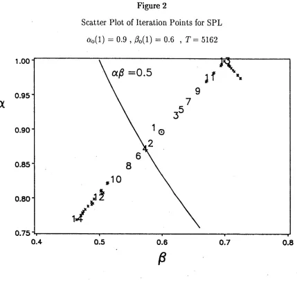
A 1.4.1 SPL Algorithm, Spliid ( 1983)

Stage I: Use (Al.2.1) or (Al.2.2) to fit an AR(h) model to yT

Obtain residual sequence t(t,91) and construct x(t,0\) as in (1.4.2) where 9\ is the estimated parameter vector of the fitted

AR(h) model

Stage II: Iterate (1.4.4), initiating with x(t,9i).

Obtain ARMA(p,q) parameter estimates 9n,n=2,3,..., updating x(t,9n-i), f(^ n -i) via (1.4.1), (1.4.2) at each iteration until convergence is achieved.

In part II, chapter 4, SPL is extensively studied (along with other algorithms that we discuss shortly) and will be dealt with in more precise detail there.

Note that by setting up a two—stage procedure no initial ARMA parameter estimate is required. If the Levinson—Durbin recursion (Al.2.1) is used in stage I, 9\(z) is guaranteed to be stable, and also h can be selected via (1.2.1). The simulation results of chapter 4 suggest that this is a better strategy than taking a fixed value of h. However, when 9\ is calculated by LS (Al.2.2), the same algorithm format is maintained in each stage. Consequently, SPL can be programmed as an iterative loop using one (variable—dimension) regression residual—update routine

call.

However, a stability problem arises in stage II, since the residuals e(t,9n) are recursively generated and therefore directly dependent on the quality of 9n. If the transfer function associated with the residual updating at stage II becomes unstable, the residuals will grow unboundedly with each successive iteration and the

algorithm will not converge. Typically, numerical overflows would cause the program to abort. Also, if the true ARMA process has near—common factors or if a

may arise, due to near pole—zero cancellations occuring in the transfer function. In this case, re—estimating or reducing the order of the ARMA model may be worthwhile.

The stability problem can be overcome by implementing a monitoring scheme in parallel with SPL. Monitoring (discussed in detail in section 4.3) ensures that the transfer function used in the residual updating is stable at each n. Alternatively SPL can be modified and this leads to algorithms which have different convergence properties. Ideally, global convergence to the (unique) limiting point 90is desired, since this removes sensitivity to the initial estimate. (Note that in our case, the initial estimate of the ARMA coefficients is given by §2) . However, global

convergence results (even though they might exist), tend to be difficult to establish and often, only local convergence results are known. By "local" convergence we mean that there exists a nondegenerate ball about 90, such that, if the 9nsequence is initiated within this ball and T is sufficiently large, then it may be shown that 9n

converges to 90. In contrast, no such initiation requirements are needed for global convergence results. Therefore, to a certain extent local results are of limited value. In either case however, conditions on the true parameters may be needed to establish convergence (in addition to the standard assumptions).

We now give two results relating to the asymptotic properties of the SPL

algorithm. We emphasize that these are the results of Stoica et al (1984) (adapted to our notation) and will be discussed in detail in chapter 4. The following matrices will be referred to:

(1.4.5) X0=S[x{t,90)x(t,90) /], Do=£[x(ti9o)uj(ti0o)']i

where u(t,90)=b0(z)~1x(t,90)and x(t,90)is just x0(t) as defined in (1.2.3)

Proposition 1.4.1 Local convergence o f SPL

The SPL estimator of 90 converges locally to 90 as T,n—►oo, iff all the

eigenvalues of X~qD0satisfy

\X(Xö1D0) - l \ < 1

where A(A) denotes an eigenvalue of a matrix A. Here, the convergence is in probability and it is also assumed that the e(t) are independent. In chapter 4 it will shown that almost sure convergence holds with (1.1.6), under a condition closely

related to (1.4.6). For p=q=l, condition (1.4.6) requires that cv0(l)ß0(l)<l/2. Thus, as pointed out by Stoica et al (1985), SPL converges under rather restrictive conditions. However, when SPL does converge, Stoica et al (1984) obtain the following Central Limit Theorem (CLT) result (also derived heuristically by Spliid,

1983).

Proposition 1.4.2 Asymptotic Normality of SPL

Let 6 denote the limit of n—>oo. Assume Proposition 1.4.1 holds and that 0 is a consistent estimator of 0O. Then

y/T{0-6o) - AN(0,HS) where

(1.4.7) = Dö'XoiDo'Y1

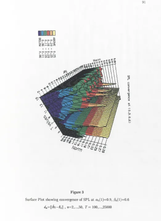
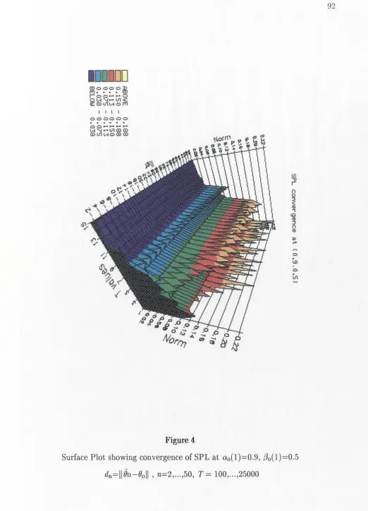
As we have said above, the asymptotic properties of the SPL procedure will be dealt with more precisely in chapter 4 and the above results rigorously established. Simulation results for the ARM A (1,1) case are also presented in chapter 4 which clearly illustrate the effect of the condition a0(l)ß0( l ) < l / 2 required for convergence and the need for modifications to the SPL procedure.

In Stoica et al (1985) a Step—Variable form of SPL is considered where a gain sequence {pn} is introduced. Thus (1.4.4b) becomes

(1-4.8) ^n+l— ^n+MnP^(^n)^rp(^n)

where the pn are assumed to satisfy,

00

(1.4.9) /in>0, lira //n=0, B? 1/*n= oo

Under (1.4.9) the condition required for local convergence is shown to be

critical. However we do not deal with the step—variable form and refer the reader to Stoica et al (1984, 1985) for further details.

An alternative which does not require monitoring is considered in Stoica et al (1985) and which we refer to as LRR (for Lagged Regression Residuals) for reasons that will become apparent.

A l.4 .2 LR R Algorithm, Stoica et al (1985)

Proceed exactly as in SPL (Al.4.1), except from n >2 on, when the residual updating (1.4.1) in Stage II is replaced by

(1.4.10) e ( t j n) = y (t)-6 n'x(t,0n-i)

Thus (1.4.10) lags (1.4.1) by one iteration. It follows that the transfer function associated with (1.4.10) is a polynomial with geometrically decreasing weights (see chapter 4) since under (1.1.5) the roots of a(zA), b(zA) are less than unity in modulus. Consequently, it should not matter if 0n+i leaves the stability region (at

least temporarily) since, asymptotically, the parameter estimates must eventually return. Hence, monitoring of the LRR algorithm is not required. LRR is also extensively studied in chapter 4 and the following convergence result is established.

Proposition 1.4.3 Restricted Global Convergence o f LRR

The LRR procedure (Al.4.2) converges globally to 0o as T,n —>oo, in a certain restricted sense, when b0(z) satisfies the positve real condition (PRC)

(1.4.11) S[260(clu,)_1- l ] > 0 , a;e[-7r,7r]

We shall explain precisely what we mean by the statement, "a certain restricted sense", in chapter 4, but it essentially refers to the fact that we have not shown 0n—>0 as asserted in Proposition 1.4.2 for SPL. Consequently, a CLT result has not been obtained for LRR, although we suspect the same limiting distribution as SPL

holds for b0(z) although the proof appears somewhat incomplete. Again, the reader is referred to chapter 4 for details.

Clearly, all the preceding algorithms depend on conditions which are essentially "uncheckable" since they relate to a true parameter 90 which is unlikely to be known or, in reality, exist. What is required is an algorithm that does not depend on such conditions and, asymptotically, will always work. (Of course, in practice,

monitoring may still be required for finite T). Such an algorithm is the three—stage procedure of Mayne and Firoozan (1978, 1982) originally suggested by Durbin (1960). Hannan and Rissanen (1982) extended this to a full identification procedure incorporating order selection and in this form, investigated the asymptotic properties of the algorithm. We shall refer to this algorithm as HR and denote the respective stages by HR(j), j=1,2,3.

Before presenting the HR algorithm we first return to the comment made earlier concerning the derivative d c ( t , 0 ) / d 0 . Recall that e ( t , 9 ) = y ( t ) - 9 / x(t,9). Thus, putting

< - ( « ( 1 ) .... «(p) Ä 1).-,/?(?))> we may write

<t,9) = J 0a - j t f l M t - j J )

Define

Then it can be seen that

(1.4.12b) K z) v ( t ) = y(t) , b(z)£(t) =

where the first term in (1.4.12b) may also be written as a(z)rj(t) = c(t,9). Clearly, given an estimate 9 of 9 , estimates of the "derivatives" in (1.4.12a) can be recursively calculated from (1.4.12b) since b(z), e{t,9) and y(t) are known. (Again, the recursion may be initiated by setting preperiod values to zero). Thus, consider

the regression of w ( t ) = c ( t , 0 ) —£ ( t ) + r j ( t ) on X2{ t ) ' = — [ d e ( t , 9 ) / 0 9 \q=q. Then since

=

c(M )-(a(z)-l

=

X2(t)'

ß = [Y,tx2(i)x2{t)/Y1[Y,iX2{t)w(t)\

= [TliX2(t)x2{t)/Y1[TliJ^(t)e(t,ß)+T,ix2(t)x2{t)'0 ] = 9 +\ZtX2(t)x2(t)/Y1\Efö(t)e(tJ)]

where E denotes the sum over 1 <t<T. This is therefore, just a Gauss—Newton iteration and constitutes HR(3). We now describe HR for given p,q.

Al.4.3 HR Algorithm (p,q known)

HR(1): Fit AR(h) by selecting h via (1.2.1) Output e(t,01) at selected h HR(2): Compute 6(2) = 6 2 from (1.4.4)

Output 62(z) and €2( ^6 2) from (1.4.1)

HR(3): Efficient Estimation

Recursively calculate rj(t), £(t) from

b2(z)rj(t)=y(t), b2(z)i(t)=c2( t j2), rj(t)=i(t)=0, t<0.

Construct, X2( t ) ' = ( - f j ( t - l ) , . . . , - r j ( t - p ) , £ ( t - l ) y. . . ^ ( t - q ) )

Regress, e2(t,02)+rj(t)-£(t) on x2(t).

Output ^(3) via (1.4.4)

It is shown by Hannan and Rissanen (1982) that 0(3) is asymptotically efficient which can be seen to be plausible by noting that - x2(t)' estimates de(t,0) / d0.

Consequently, HR(3) corresponds to one iteration of a Gauss—Newton procedure to optimize the concentrated likelihood function Cc(0) given by (1.3.11). (For a more detailed discussion of the Gauss—Newton procedure with respect to HR see Kavalieris, 1984 and Hannan and Deistler, 1988). Although there can be no

Proposition 1.4.4 Asymptotic Properties of HR Algorithm A For HR(2), 0(2)—>90 a.s. and

(1.4.13) VT(0(2)-0O)~ AA(0,ftH)

where ft., is derived in chapter 4.

H

B For HR(3), 0(3)—>0O a.s. and

VT(0(3)-0O)~ ANiO&ö1)

where ft0 is given by (1.3.14) and is exactly Xöl of (1.4.5).

In chapter 4, the CLT result (1.4.13) for HR(2) is established and the remaining results in Proposition 1.4.4 are established in Hannan and Rissanen (1982), and Hannan and Kavalieris (1984a), the latter reference dealing with the vector form of HR. However, it is also shown in chapter 4, that

where ft is given in (1.4.7). Thus, it follows that, asymptotically, no gain is

o

obtained from iterating (1-4-4) in the SPL procedure. For finite T however, there will be differences between HR, SPL and LRR and these are investigated through the simulation studies carried out in chapter 4. Since HR can be used as full identification procedure, it is appropriate that we turn to the problem of order selection in the following section.

§1.5 Order Selection

The consistency results stated in the previous sections only apply when the true order of the ARMA system is known. However, for the identification problems we consider here, the order will not be known a priori and needs to be estimated.

In the Box and Jenkins (1970) approach, the sample correlogram is used to determine the order. Extensions to this approach have been considered by Chatfield

is because these techniques depend, to a certain extent, on pattern recognition which is subjective. Consequently, it would be difficult to study these techniques analytically and also, the user interaction required would preclude their use in online situations. Note however, that the correlogram is an important diagnostic tool for detecting seasonal and trend characteristics.

Since the selection of order corresponds to model estimation over a

variable-dimensioned parameter space, direct use of the maximum likelihood principle invariably leads to the highest possible order being selected. This cannot therefore provide consistent estimates and is in conflict with the intuitive notion of selecting an appropriate order. The analogous situation is encountered in standard regression analysis for the selection of regressor variables. There, the residual sum of squares decreases monotonically as the number of variables included in the regression increases.

An extension to the maximum likelihood principle was introduced in Akaike (1972) in terms of an information criterion of the form of (1.2.1) called AIC (below). Other criteria have since followed and two special cases of importance are

(1.5.1) AIC{h)=log dg +h2/ T , BIC{h)=log dg + /ilo g T /T

Here, dg is the MLE of al from a model of order h. BIC was introduced in Akaike (1977) and has been justified on a Bayesian basis by Schwartz (1978) and on

another basis by Rissanen (1983). Akaike (1969) had in fact, earlier considered a criterion asymptotically identical to AIC in the context of fitting autoregressions. However, as suggested by Akaike (1974), these criteria can be applied to the more general problem of choosing among different models (not necessarily time series) with different numbers of parameters. See for example, Sakamoto, Ishiguro and Kitagawa (1986) where AIC is used in a wide variety of statistical applications.

To emphasise order selection for the ARM A case we rewrite (1.2.1) as (1.5.2) log dg,q+{p+q)C(T)/T, p<P, q<Q

minimize (1.5.2). Assume that the true orders satisfy Po<P,q0<Q- A characteristic of (1.5.2) is that to determine p0 and q0, orders greater than the true orders need to be examined. Problems now arise, both numerically and with the asymptotic theory, since the parameter vector 0 (of dimension p+q) does not converge in any reasonable

sense. This is because the likelihood function is constant along the line where ap(z)bq(z)~1=a0{z)b0(z)~1 so that as T increases the extra zeros, nearly common to aP(z),bq(z), converge to \z\= l in an erratic manner thus causing 0 to fluctuate between sample points close to this line. An example of this type of behaviour is discussed in Hannan and Deistler (1988, section 5.4). Consequently, it is necessary to strengthen (1.1.5) to the following

(1.5.3) a0(z),b0(z) coprime and öo(^)/0, |^|<1, öo(^)/0, |2r|<l-h^, <^>0

for S known a priori. This ensures the zeros of b0(z) are bounded away from | z\ =1. The following theorem is due to Hannan (1980), but uses the results of An, Chen and Hannan (1982) to remove the assumption of independence on the e(t) sequence. Theorem 1.5.1 Consistency o f(1.5.2)

Let p,q be the minimizing values obtained from (1.5.2) assuming p0<P, qo<Q is known. Assume (1.5.3) is known to hold and let (1.1.6) hold for the e(t). Then there are co,ci, 0<co < ci<oo such that the following are true:

(i) If liminf {C(T)/21og logT}>ci then ( p ,q)—>(p0,q0) a.s. (ii) If limsup {C(71)/21og logT}<co then (i) fails

(hi) If C( T)—>oo then (p,q)-*->

(p0,?o)-(iv) If limsup C(T)<oo then (iii) fails unless P=p0,

Q=qo-If £[e(t)2|7t-i]=0o is assumed, as in (1.1.6), co,ci may be taken as 1 in the above. (By relaxing this condition, Theorem 1.5.1 can be shown to hold for P,Q depending

Corollary 1.5.1

Let the conditions of Theorem 1.5.1 hold. Assume p0<P, qo<Q and

limsup C(T)<oo. Then

lim 1 im ?[p >p0,q >q0]=l Ö+0 T-+00

This result clearly shows that AIC does not provide consistent order estimates and is also certain to overestimate the orders. The same conclusion is also true if one of

Po—P or q0=Q, is used in Corollary 1.5.1. In particular, if q0=Q=0, p0<P, so that

AIC cannot consistently estimate the true order of an AR process. Indeed, Shibata (1976) showed, for a Gaussian AR process of finite true order p0, that using the AIC procedure will overestimate the true order with non—zero probability.

However, while these asymptotic results would appear to distinctly favour BIC over AIC for example, there will be more chance, for fixed T, of underestimating the order the larger C( T) is taken. Thus, it is of interest to find a C(T) increasing with T as slowly as possible yet still giving consistent order estimates. As can be seen from Theorem 1.5.1 strong consistency eventually holds to the accuracy of the law of the iterated logarithm (LIL). That is for C( T)=cloglogT, c>2 under (1.1.6). This result was established by Hannan and Quinn (1979) in the context of autoregressive processes but as pointed out by these authors (op. cit. pl93) the LIL can hardly be viewed as operating for small T. Thus in effect, loglog T increases too slowly for the asymptotic theory to have much meaning.