Point-Based Planning for Multi-Objective POMDPs

Point-Based Planning for Multi-Objective POMDPs

Diederik M. Roijers

, Shimon Whiteson

,

and

Frans A. Oliehoek

_{Informatics Institute, University of Amsterdam, The Netherlands}

_{Department of Computer Science, University of Liverpool, United Kingdom}

{

d.m.roijers, s.a.whiteson, f.a.oliehoek

}

@uva.nl

Abstract

Many sequential decision-making problems require an agent to reason about both multiple objec-tives and uncertainty regarding the environment’s state. Such problems can be naturally modelled as multi-objective partially observable Markov deci-sion processes (MOPOMDPs). We propose opti-mistic linear support with alpha reuse (OLSAR), which computes a bounded approximation of the optimal solution set for all possible weightings of the objectives. The main idea is to solve a series of scalarized single-objective POMDPs, each cor-responding to a different weighting of the objec-tives. A key insight underlying OLSAR is that the policies and value functions produced when solv-ing scalarized POMDPs in earlier iterations can be reused to more quickly solve scalarized POMDPs in later iterations. We show experimentally that OLSAR outperforms, both in terms of runtime and approximation quality, alternative methods and a variant of OLSAR that does not leverage reuse.

1

Introduction

Many real-world planning problems require reasoning about incomplete knowledge of the environment’s state. These problems are often naturally modelled as partially observ-able Markov decision processes (POMDPs)[Kaelblinget al., 1998]. Since optimal POMDP planning is intractable, much research focusses on efficient approximations.

However, planning is often further complicated by the presence of multiple objectives. For example, an agent might want to maximize the performance of a computer network while minimizing its power consumption [Tesauro et al., 2007]. Such problems can be modeled asmulti-objective par-tially observable Markov decision processes (MOPOMDPs) [Soh and Demiris, 2011a; 2011b].

Solving MOPOMDPs does not always require special so-lution methods. For example, when the vector-valued reward function can bescalarized, i.e., converted to a scalar function, before planning, the original problem may be solvable with existing single-objective methods. Unfortunately, a priori scalarization is not possible when thescalarization weights,

i.e., the parameters of the scalarization, are not known in ad-vance. For example, a company that produces different re-sources whose market prices vary may not have enough time to re-solve the decision problem for each price change. In such cases, multi-objective methods are needed to compute a set of solutions optimal for all scalarizations.

Little research has been conducted on such methods for MOPOMDPs. A naive approach is to translate the MOPOMDP to a single-objective POMDP with an aug-mented state space that includes as a feature a single, hid-den “true” objective; a similar approach has been proposed for MOMDPs [White and Kim, 1980]. However, this ap-proach precludes the use of POMDP methods that exploit an initial belief (such as point-based methods [Shaniet al., 2013]) since specifying an initial belief fixes the scalarization weights. Another naive approach is to uniformly randomly sample scalarization weights and then solve each resulting scalarized problem with a single-objective POMDP planner. Unfortunately, this requires a large amount of sampling to get good coverage of the space of scalarization weights.

In this paper, we propose a new MOPOMDP solution method calledoptimistic linear support with alpha reuse (OL-SAR). Our approach is based on optimistic linear support (OLS)[Roijerset al., 2014a; 2015], a general framework for solving multi-objective decision problems that uses a priority queue to make smart choices about which scalarized problem instances to solve.

OLSAR contains two key improvements over OLS that are essential to making it tractable for MOPOMDPs. First, it uses a novelOLSAR-compliantversion of the point-based solverPerseus[Spaan and Vlassis, 2005]. OLSAR-compliant Perseus solves a given scalarized POMDP and simultane-ously computes the resulting policy’smulti-objectivevalue. Doing so avoids the need for the separate policy evalua-tion step typically employed by OLS [Roijerset al., 2014b]. Since POMDP policy evaluation is very expensive, the use of OLSAR-compliant Perseus is key to OLSAR’s efficiency. Second, rather than solving each scalarized POMDP from scratch, OLSAR reuses the α-matrices that represent each policy’s multi-objective value to form an initial lower bound for subsequent calls to OLSAR-compliant Perseus. Such reuse leads to dramatic reductions in runtime in practice.

initial belief but does not require inefficient sampling of the scalarization weight space.

We show that OLSAR is guaranteed to find a bounded ap-proximate solution in a finite number of iterations. In addi-tion, we show experimentally that it outperforms uniform ran-dom sampling of scalarization weights, both with and without

α-matrix reuse, as well as OLS withoutα-matrix reuse.

2

Background

We start with background on multi-objective decision prob-lems, POMDPs, MOPOMDPs, and OLS.

2.1

Multi-Objective Decision Problems

In single-objective decision problems, an agent must find a policyπthat maximizesV, the expected value of, e.g., a sum of discounted rewards. In multi-objective decision problems, there arenobjectives, yielding a vector-valued reward func-tion. As a result, each policy has a vector-valued expected valueVand, rather than having a single optimal policy, there can be multiple policies whose value vectors are optimal for different preferences over the objectives. Such preferences can be expressed using a scalarization functionf(V,w)that is parameterized by a parameter vector w and returnsVw,

the scalarized value ofV. Whenw is known beforehand, it may be possible toa prioriscalarize the decision problem and apply standard single-objective solvers. However, when

w is unknown during planning, we need an algorithm that computes a set of policies containing at least one policy with maximal scalarized value foreach possiblew.

Which policies should be included in this set depends on what we know aboutf, as well as which policies are allowed. In many real-world problems,fis linear, i.e.,

f(V,w) =w·V,

wherewis a vector of non-negative weights that sum to 1. In this case, a sufficient solution is theconvex hull (CH), the set of all undominated policies under a linear scalarization:

CH(Π) ={π:π∈Π∧ ∃w∀(π0∈Π)w·Vπ≥w·Vπ0}, (1)

whereΠ is the set of allowed policies. However, the entire CH may not be necessary. Instead, it also suffices to compute aconvex coverage set (CCS), a lossless subset of the CH. For each possiblew, a CCS contains at least one vector from the CH that has the maximal scalarized value forw.

Whenf is not linear, we might require the Pareto front (PF), a superset of the CH containing all policies for which no other policy has a value that is at least equal in all objec-tives and greater in at least one objective. However, when stochastic policiesare allowed, all values on the PF can be constructed from mixtures of CCS policies [Vamplewet al., 2009]. Therefore, the CCS is inadequate only if the scalariza-tion funcscalariza-tion is nonlinearandstochastic policies are forbid-den. For simplicity, we assume linear scalarizations in this paper. However, our methods are also applicable to nonlinear scalarizations as long as stochastic policies are allowed.

Using the CCS, we can define ascalarized value function:

V_CCS∗ (w) = max

V∈CCSw·V, (2)

which returns, for each w, the maximal scalarized value achievable for that weight. Finding this function is equiv-alent to finding the CCS and solving the decision problem.

V_CCS∗ (w)is apiecewise-linear and convex (PWLC)function over weight space, a property that can be exploited to con-struct a CCS efficiently [Roijerset al., 2014a; 2015].

When the CCS cannot be computed exactly, anε-CCS can be computed instead. A setXis anε-CCS is when the maxi-mum scalarized error across all weights is at mostε:

∀w, VCCS∗ (w)−(max

V∈Xw·V)≤ε. (3)

2.2

POMDPs

An infinite-horizon single-objective POMDP [Kaelbling et al., 1998; Madaniet al., 2003] is a sequential decision prob-lem that incorporates uncertainty about the state of the en-vironment, and is specified as a tuple hS, A, R, T,Ω, O, γi

whereS is the state space; A is the action space; R is the reward function;Tis the transition function, giving the prob-ability of a next state given an action and a current state;Ωis the set of observations;Ois the observation function, giving the probability of each observation given an action and the resulting state; andγis the discount factor.

Typically, an agent maintains a beliefbover which state it is in. The value function for a single-objective POMDP,Vb, is

defined in terms of this belief and can be represented by a set

Aofα-vectors. Each vectorα(of length|S|) gives a value for each states. The value of a beliefbgivenAis:

Vb= max

α∈Ab·α. (4)

Eachα-vector is associated with an action. Therefore, a set ofα-vectorsAalso provides apolicyπAthat for each belief

takes the maximizing action in (4).

While infinite-horizon POMDPs are in general undecid-able [Madaniet al., 2003], anε-approximate value function can in principle be computed using techniques likevalue iter-ation (VI) [Monahan, 1982] andincremental pruning [Cas-sandra et al., 1997]. Unfortunately, these methods scale poorly in the number of states. However,point-based meth-ods [Shaniet al., 2013], which perform approximate backups by computing the bestα-vector only for a setBof sampled beliefs, scale much better. For eachb ∈ B, apoint-based backupis performed by first computing for eachaando, the back-projectiong_ia,oof each next-stage value vectorαi∈ Ak:

g_ia,o(s) = X s0_∈S

O(a, s0, o)T(s, a, s0)αi(s0). (5)

This step is identical for (and can be shared amongst) allb∈

B. For eachb, the back-projected vectors g_ia,o are used to construct|A|newα-vectors (one for each action):

αb,a_k+1=ra+γX

o∈Ω

arg max ga,o

b·ga,o, (6)

where ra is a vector containing the immediate rewards for performing actionain each state. Finally, theαb,a_k+1that max-imizes the inner product withb(cf. (4)) is retained as the new

α-vector forb:

backup(Ak, b) = arg max αb,a_k+1

Point-based methods typically perform several point-based backups usingAk for different b to construct the set ofα

-vectors for the next iteration,Ak+1. By constructing theα

-vectors only from thega,o_{that are maximizing for the given}

b, point-based methods avoid generating the much larger set ofα-vectors that an exhaustive backup ofAkwould generate.

2.3

MOPOMDPs

A MOPOMDP [Soh and Demiris, 2011b] is a POMDP with a vector-valued reward functionR instead of a scalar one. The value of a MOPOMDP policy given an initial beliefb0is

thus also a vectorVb0. The scalarized value givenwis then

w·Vb0. Note that in an MOPOMDP, a nonlinear scalarization

would make it impossible to construct a POMDP model for a particularw, since a nonlinearf does not distribute over the expected sum of rewards. Therefore, nonlinear scalarization would preclude the application of dynamic-programming-based POMDP methods [Roijerset al., 2013].

BecauseRis vector valued, each element of eachα-vector, i.e., eachα(s), is itself a vector, indicating the value in all objectives. Thus, each α-vector is actually an α-matrix A

in which each rowA(s)represents the multi-objective value vector fors. The multi-objective value of taking the action associated withAunder beliefb(provided as a row vector) is thenbA. Whenw is also given (as a column vector), the scalarized value of taking the action associated withAunder beliefbisbAw. Given a set ofα-matricesAthat approxi-mates the multi-objective value function, we can thus extract the scalar value given a beliefbfor everyw:

Vb(w) = max

A∈A bAw. (8)

Since eachα-matrix is associated with a certain action, a pol-icyπ_Awcan be distilled fromAgivenw. The multi-objective value for a givenb0under policyπis denotedVbπ0 =b0A.

A naive approach to solving MOMDPs, which we refer to asrandom sampling (RS)[Roijerset al., 2014b], was intro-duced in the context of multi-objective MDPs. RS samples manyw’s and creates a scalarized POMDP according to each

w. Unless some prior knowledge aboutwis available, sam-pling is uniformly random. Each scalarized POMDP can then be solved with any POMDP method, including point-based ones. The resulting multi-objective value vectors are main-tained in a setX, which forms a lower bound on the scalar-ized value function:

V_X∗(w) = max V∈Xw·V.

An important downside of this method is that althoughXwill converge to the CCS in the limit, we do not know when this is the case. Furthermore, becauseware sampled at random, RS might do a lot of unnecessary work.

2.4

Optimistic Linear Support

This paper builds onoptimistic linear support (OLS)[Roijers et al., 2014a; 2015] — a general scheme for solving multi-objective decision problems. Like RS, OLS repeatedly calls a single-objective solver to solve scalarized instances of the multi-objective problem and maintains a setX that forms a lower bound on the value functionV_X∗(w). Contrary to RS

0.0 0.2 0.4 0.6 0.8 1.0

0

2

4

6

8

w1

Vw

Δ

wc

(1,8)

(7,2)

0.0 0.2 0.4 0.6 0.8 1.0

0

2

4

6

8

w1 Vw

(1,8)

(7,2) (5,6)

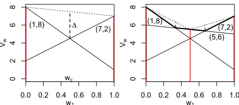
Figure 1: Finding value vectors, corner weights, and the max-imal possible improvement for a partial CCSXin OLS.

however, OLS selects the weight vectorswinstances intelli-gently. In order to select goodw’s for scalarization, OLS ex-ploits the observation thatV_X∗(w)is PWLC over the weight simplex. In particular, OLS selects only so-called corner weightsthat lie at the intersections of line segments of the PWLC functionV_X∗(w)that correspond to the value vectors found so far. OLS prioritizes these corner weights according to an optimistic estimate of their potential error reduction.

First, let us assume OLS has access to an optimal single-objective solver. For this case, the workings of OLS are il-lustrated for a 2-objective problem in Figure 1. The first corner weights (denoted with red vertical line segments) are the extrema of the weight simplex. On the left, OLS finds an optimal value vector for both extrema: (1,8)and(7,2). After finding these first two value vectors, OLS identifies a new corner weight: wc. At this corner weight, the maxi-mal possible improvement consistent with scalarized values found at the extrema of the weight simplex is∆. OLS now calls the single-objective solver forwc, and discovers a new value vector,(5,6), leading to two new corner weights. OLS first processes the corner weight with the largest∆, which is an optimistic estimate of the error reduction that processing that corner weight will yield. In Figure 1 (right), OLS selects the corner weight on the right, because its maximal possible improvement,∆, is highest.

If no improving value vector for a corner weight is found by the single-objective solver, the value for that corner weight is optimal, and no new corner weights are generated. When none of the remaining corner weights yield an improvement, the intermediate setX is a CCS and OLS terminates.

When the single-objective solver is exact, OLS is thus guaranteed to produce an exact CCS after a finite number of calls to the single-objective solver. Furthermore, even when a bounded approximate single-objective solver is used instead, OLS retains this quality bound.

Lemma 1. Given anε-optimal approximate single-objective solver, OLS produces anε-CCS [Roijerset al., 2014b].

3

OLS with Alpha Reuse

Algorithm 1:OLSAR(b0, η)

Input: A POMDP

1 X← ∅; // partial CCS of multi-objective value vectorsVb0

2 W Vold← ∅; // searched weights and scalarized values

3 Q←priority queue with weights to search;

4 Add extrema of the weight simplex toQwith infinite priority;

5 Aall←a set ofα-matrices forming a lower bound on the value;

6 B←set of sampled belief points (e.g., by random exploration);

7 while¬Q.isEmpty()∧ ¬timeOutdo

8 w←Q.dequeue(); // Retrieve a weight vector

9 Ar←select the bestAfromAallfor eachb∈B, givenw; 10 Aw←solveScalarizedPOMDP(Ar, B,w, η);

11 Vb0←maxA∈Awb0Aw;

12 Aall← Aall∪ Aw;

13 W Vold=W Vold∪ {(w, w·Vb0)};

14 ifVb06∈Xthen

15 X←X∪ {Vb0};

16 W ←compute new corner weights and maximum possible improvements(w,∆w)usingW VoldandX; 17 Q.addAll(W);

18 end

19 end

20 returnX;

iterations, OLSAR greatly speeds up later iterations. Second, by using anOLSAR-compliantpoint-based solver as a sub-routine, it obviates the need for separate policy evaluations.

We first describe OLSAR and specify the criteria that the single-objective POMDP method that OLSAR calls as a sub-routine, which we call solveScalarizedPOMDP, must sat-isfy to be OLSAR-compliant. Then, Section 3.1 describes an instantiation of solveScalarizedPOMDP that we call OLSAR-Compliant Perseus. Finally, Section 3.2 discusses OLSAR’s theoretical properties, which leverage existing the-oretical guarantees of point-based methods and OLS.

OLSAR maintains an approximateCCS,X, and thereby an approximate scalarized value function V_X∗. By extend-ing X with new value vectorsVb₀,V_X∗ approaches V_CCS∗ . The vectorsVb0are computed using sets ofα-matrices.

OL-SAR finds these sets of α-matrices by solving a series of scalarized problems, each of which is a decision problem over belief space for a different weight w. Each scalar-ized problem is solved by a single-objective solver we call

solveScalarizedPOMDP, which computes the value

func-tion of the MOPOMDP scalarized byw.

OLSAR, given in Algorithm 1, takes an initial beliefb0

and a convergence threshold η as input. The value vec-tors Vb0 found for differentw are kept in a partial

approx-imate CCS, X (line 1). OLSAR keeps track of which w

have been searched and the associated scalarized values in a set of tuplesW Vold (line 2). The weights that still need

to be investigated are kept in a priority queueQ, and priori-tized by their maximal possible improvement∆w(lines 3–4),

which is calculated via a linear program [Roijerset al., 2014a; 2015]. OLSAR also maintainsAall, a set of allα-matrices

re-turned by calls tosolveScalarizedPOMDPto reuse (line 5) andB, a set of sampled beliefs (line 6).

In the main loop, (lines 7–18) OLSAR repeatly pops a cor-ner weight off the queue. For each poppedw, it selects the

α-matrices fromAallto initializeAr, a set ofα-matrices that

form a lower bound on the (multi-objective) value (line 9). Initially, this lower bound is a heuristic lower bound. In the single-objective case, this usually consists of a minimally re-alisable value heuristic, in the form ofα-vectors. In order to enableα-reuse for the multi-objective version, these heuris-tics must be in the form ofα-matrices. For example, if we denote the minimal reward for each objectiveiasRi

min, one

lower bound heuristicα-matrixAminis the vectors consist-ing ofRi

min/(1−γ)for each objective and state.

OLSAR selects the maximizingα-matrix (2) for each be-liefb∈Band the givenwand puts them in a setAr. Using Ar, OLSAR callssolveScalarizedPOMDP. After obtaining

a new set ofα-matricesAwfromsolveScalarizedPOMDP,

OLSAR calculates Vb0; the maximizing multi-objective

value vector forb0 atw(line 11). IfVb0 is an improvement

toX (line 14), OLSAR adds it toX and calculates the new corner weights and their priorities.

A key insight behind OLSAR is that if we can re-trieve the α-matrices underlying the policy found by

solveScalarizedPOMDP for a specific w, we can reuse

theseα-matrices as a lower bound for subsequent calls to

solveScalarizedPOMDP with another weight w0.

Espe-cially whenwandw0are similar, we expect this lower bound to be close to theα-matrices required forw0.

However, to exploit this insight,solveScalarizedPOMDP

must return the α-matrices explicitly, not just the scalar-ized value or the single-objective α-vectors, as standard single-objective solvers do. A naive way to retrieve theα -matrices is to perform a separate policy evaluation on the pol-icy returned bysolveScalarizedPOMDP. However, since POMDP policy evaluation is expensive, we instead require

solveScalarizedPOMDPto be OLSAR-compliant: i.e., to

return a set ofα-matrices, while computing the same scalar-ized value function as a single-objective solver. We propose an OLSAR-compliant solver in Section 3.1.

Theα-matrix reuse enabled by an OLSAR-compliant sub-routine is key to solving MOPOMDPs efficiently. Intuitively, the corner weights that OLSAR selects lie increasingly closer together as the algorithm iterates. Consequently, the poli-cies and value functions computed for those weights lie closer together as well andsolveScalarizedPOMDPneeds less and less time to improve upon theα-matrices that be-gin increasingly close to their converged values. In fact, late in the execution of OLSAR, corner weights are tested that yield no value improvement, i.e., no new α-matrices are found. These tests serve only to confirm that the CCS has been found, rather than to improve it. While such confirmation tests would be expensive in OLS, in OLSAR they are trivial: the already presentα-matrices suffice and

solveScalarizedPOMDP converges immediately. As we

show in Section 4, this greatly reduces OLSAR’s runtime.

3.1

OLSAR-Compliant Perseus

OLSAR requires an OLSAR-compliant implementation of

solveScalarizedPOMDP that returns the multi-objective

value of the policy found for a givenw. This requires redefin-ing the point-based backup such that it returns anα-matrix rather than anα-vector. Starting from a set ofα-matricesAk,

Algorithm 2:OCPerseus(A, B,w, η)

Input: A POMDP 1 A0← A;

2 A ← {−∞}~ ; // worst possible vector in a singleton set

3 whilemaxbmaxA0∈A0bA0w−(maxA∈AbAw)> ηdo

4 A ← A0;A0← ∅;B0←B;

5 whileB06=∅do

6 Randomly selectbfrom B’;

7 A←backupMO(A, b,w);

8 A0← A0∪ { arg max A0_∈(A∪{A})bA

0 w};

9 B0← {b∈B0: max A0∈A0bA

0

w<max A∈AbAw};

10 end

11 end

12 returnA0;

new backup first computes the back-projectionsGa,o_i (for all

a, o) of each next-stageα-matrixAi ∈ Ak. However, these Ga,o_i are now matrices instead of vectors:

Ga,o_i (s) = X s0_∈S

O(a, s0, o)T(s, a, s0)Ai(s0). (9)

As before, the back-projected matricesGa,o_i are identical for (and can be shared amongst) allb∈ B. For the givenband

w, the back-projected matrices are used to construct|A|new

α-matrices (one for each action):

Ab,a_k+1=ra+γX

o∈Ω

arg max Ga,o

bGa,ow. (10)

Note that the vectorsGa,ow can also be shared between all

b∈B. Therefore, we cache the values ofGa,o_w.

Finally, the Ab,a_k+1 that maximizes the scalarized value givenbandwis selected by thebackupMOoperator:

backupMO(Ak, b,w) = arg max Ab,a_k+1

bAa,b_k+1w. (11)

We can plugbackupMOinto any point-based method. In this paper, we use Perseus [Spaan and Vlassis, 2005] because it is fast and can handle large sampled belief sets. The re-sulting OLSAR-compliant Persues is given in Algorithm 2. It takes as input an initial lower boundAon the value function in the form of a set ofα-matrices, a set of sampled beliefs, a scalarization weightw, and a precision parameterη. It re-peatedly improves this lower bound (lines 3-10) by finding an improvingα-matrix for each sampled belief. To do so, it selects a random belief from the set of sampled beliefs (line 6) and, if possible, finds an improvingAfor it (line 7). When such anα-matrix also improves the value for another belief point inB, this belief point is ignored until the next iteration (line 9). This results in an algorithm that generates fewα -matrices in early iterations, but improves the lower bound on the value function, and gets more precise, i.e., generates more

α-matrices, in later iterations.

3.2

Analysis

Point-based methods like Perseus have guarantees on the quality of the approximation. These guarantees depend on

the density δB of the sampled belief set, i.e., the maximal

distance from the closest b ∈ B to any other belief in the belief set [Pineauet al., 2006].

Lemma 2. The error εon the lower bound of the value of an infinite-horizon POMDP after convergence of point-based methods is:

ε≤ δB(Rmax−Rmin)

(1−γ)2 , (12)

whereRmaxandRminare the maximal and minimal possible immediate rewards [Pineauet al., 2006].

Using Lemma 2 we can bound the error of the approximate CCS computed by OLSAR.

Theorem 1. OLSAR implemented withOCPerseususing be-lief setB converges in a finite number of iterations to anε -CCS, whereε≤ δB(Rmax−Rmin)

(1−γ)2 .

Proof. Because OLSAR follows the same iterative pro-cess as OLS, Lemma 1 applies to it, i.e., it converges after fi-nite calls tosolveScalarizedPOMDP. BecauseOCPerseus

differs from regular Perseus only in that it returns the multi-objective value rather than just the scalarized value, Lemma 2 also holds for OCPerseus for any w. In other words,

OCPerseusis anε-approximate single-objective solver, with

εas specified by Lemma 2. Therefore, it follows that OLSAR produces anε-CCS.

A nice property of OLSAR is thus that it inherits any qual-ity guarantees of thesolveScalarizedPOMDP implementa-tion it uses. Better initializaimplementa-tion of OCPerseus due to α -matrix reuse does not effect the guarantees in any way. On the contrary, it affects only empirical runtimes. The next section presents experimental results that measure these runtimes.

4

Experiments

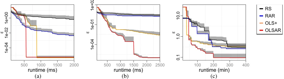
In this section, we empirically compare OLSAR to three baseline algorithms. The first is random sampling (RS), described in Section 2.3, which does not use OLS or alpha reuse. The second is random sampling with al-pha reuse (RAR), which does not use OLS. The third is OLS+OCPerseus, which does not use alpha reuse. We tested the algorithms on three MOPOMDPs based on the Tiger [Cassandra et al., 1994] and Maze20 [Hauskrecht, 2000] benchmark POMDPs. Because we use infinite-horizon MOPOMDPs – which are undecidable – we cannot obtain the true CCS. Therefore, we compare our algorithms’ solutions to reference setsobtained by running OLSAR with many more sampled belief points andηset 10 times smaller.

4.1

Multi-Objective Tiger Problem

While the single-objective Tiger problem assumes all three rewards are on the same scale, it is actually difficult in prac-tice to quantify the trade-offs between, e.g., risking an en-counter with the tiger and acquiring treasure. Intwo-objective MO-Tiger (Tiger2), we assume that the treasure and the cost of listening are on the same scale but treat avoiding the tiger as a separate objective. Inthree-objective MO-Tiger (Tiger3), we treat all three forms of reward as separate objectives.

We conducted 25 runs of each method on both Tiger2 and Tiger3. We ran all algorithms with 100 belief points gener-ated by random exploration,η = 1×10−6, andb0 set to a

uniform distribution. The reference set was obtained using

250belief points.

On Tiger2 (Figure 2(a)), OLS+OCPerseus converges in

0.87son average, with a maximal error in scalarized value across the weight simplex w.r.t. the reference set of5×10−6. OLSAR converges significantly faster (t-test: p < 0.01), in on average0.53s, with similar error4×10−6_{(this difference}

in error is not significant). RAR does not converge as it just keeps sampling new weights. However, we can measure er-ror w.r.t. the reference set. After2s(about four times what OLSAR needs to converge), RAR has an error with respect to the reference set of4.5×10−3(a factor of103higher than OLSAR after convergence). RS is even worse and does not come further than a0.78error after2s. OLS+OCPerseus and OLSAR perform similarly in the first half: they use about the same time on the first four iterations (0.35s). However, OLSAR is significantly faster for the second half. Thus, on Tiger2, OLS-based methods are significantly better than ran-dom sampling and alpha reuse significantly speeds the dis-covery of good value vectors.

The results for the Tiger3 problem are in Figure 2(b). RS and RAR both perform poorly, with RAR better by a fac-tor of two. OLS+OCPerseus is faster than RAR but OLSAR is the fastest and converges in about 2s. OLS+OCPerseus eventually converges to the same error but takes 10 times longer. As before, OLS-based methods outperform random sampling. Furthermore, for this 3-objective problem, alpha reuse speeds convergence of OLSAR by an order of magni-tude.

4.2

Multi-Objective Maze20 Problem

In Maze20 [Hauskrecht, 2000], a robot must navigate through a 20-state maze. It has four actions to move in the cardinal directions, plus two sensing actions to perceive walls in the north-south or east-west directions. Transitions and observa-tions are stochastic. In the single-objective problem, the agent gets reward of 2 for sensing, 4 for moving while avoiding the wall, and 150 for reaching the goal. Inmulti-objective Maze 20 (MO-Maze20), the reward for reaching the goal is treated as a separate objective, yielding a two-objective problem.

To test performance of OLSAR on MO-Maze20, we first created a reference set by letting OLSAR converge using 1500 sampled beliefs. This took 11 hours. Then we ran OL-SAR, OLS+OCPerseus, RAR, and RS with 1000 sampled beliefs. Due to the computational expense, we conducted only three runs per method. Figure 2(c) shows the results. OLSAR converges after (on average)291minutes (4.90hrs) at an error of 0.09, less than 0.5% w.r.t. the reference set.

We let OLS+COPerseus run for 11 hours but it did not con-verge in that time. OLS+OCPerseus, RS, and RAR have sim-ilar performance after around 300 minutes. However, until then, OLS+OCPerseus does better (and unlike RS and RAR, OLS+OCPerseus is guaranteed to converge). OLSAR con-verges at significantly less error than what the other methods have attained after 400 minutes. We therefore conclude that OLSAR reduces error more quickly than the other algorithms and converges faster than OLS+OCPerseus.

5

Related Work

As previously mentioned, little research has been done on the subject of MOPOMDPs. White and Kim (1980) proposed a method to translate a multi-objective MDP into a POMDP, which can also be applied to a MOPOMDP and yields a single-objective POMDP. Intuitively, this translation assumes there is only one “true” objective. Since the agent does not know which objective is the true one, this yields a single-objective POMDP whose state is a tuple hs, diwhere s is the original MOPOMDP state and d ∈ {1. . . n} indicates the true objective. The POMDP’s state space is of size|S|n. The observations provide information aboutsbut not aboutd. The resulting POMDP can be solved with standard methods but only those that do not require an initial belief, as such a belief would fix not only a distribution oversbut also overd, yielding a policy optimal only for a givenw. Since this pre-cludes efficient solvers like point-based methods, it is a severe limitation. We tested this method, and it proved prohibitively computationally expensive for even the smallest problems.

Other research on MOPOMDPs [Soh and Demiris, 2011a; 2011b] uses evolutionary methods to approximate the PF. However, no guarantees can be given on the quality of the ap-proximation. Furthermore, as discussed in Section 2.1, find-ing a PF is only necessary when the scalarization function is nonlinear and stochastic policies are forbidden. In this paper, we focus on finding bounded approximations of the CCS.

6

Conclusions & Future Work

In this paper we proposed, analyzed, and tested OLSAR, a novel algorithm for MOPOMDPs that intelligently selects a sequence of scalarized POMDPs to solve. OLSAR uses OCPerseus, a scalarized MOPOMDP solver that returns the multi-objective value of the policies it finds, as well as the

α-matrices that describe them. A key insight underlying OL-SAR is that these α-matrices can be reused in subsequent calls to OCPerseus, greatly reducing runtimes in practice. Furthermore, since OCPerseus returnsε-optimal polcies, OL-SAR is guaranteed in turn to return an ε-CCS. Finally, our experiments results show that OLSAR greatly outperforms alternatives that do not use OLS and/orα-matrix reuse.

1e

-0

4

1e

-0

2

1e

+0

0

500 1000 1500 2000

runtime (ms)

ε

1e

-0

4

1e

-0

1

1e

+0

2

500 1000 1500 2000 2500

runtime (ms)

ε

0.1

1.0

10.0

100 200 300 400

runtime (min)

ε

(a) (b) (c)

Figure 2: The error with respect to a reference set as a function of the runtime for (a) Tiger 2, (b) Tiger3, and (c) MO-Maze20. The shaded regions represent standard error. Note the log scale in they-axis. In order to avoid clutter in the plot (due to the log-scale) we only show the standard error above the lines.

corresponds to the solution of an MOPOMDP linearly scalar-ized according to somew[Poupartet al., 2015]. Using this result, we aim to investigate how anε-CCS computed by OL-SAR could be used to explore what sets of constraints are feasible in a CPOMDP.

Acknowledgments

This research is supported by NWO DTC-NCAP (#612.001.109) project and the NWO Innovational Re-search Incentives Scheme Veni (#639.021.336).

References

[Cassandraet al., 1994] A.R. Cassandra, L.P. Kaelbling, and M.L. Littman. Acting optimally in partially observable stochastic do-mains. InAAAI, volume 94, pages 1023–1028, 1994.

[Cassandraet al., 1997] A.R. Cassandra, M.L. Littman, and N.L. Zhang. Incremental pruning: A simple, fast, exact method for partially observable Markov decision processes. InUAI, pages 54–61, 1997.

[Hauskrecht, 2000] M. Hauskrecht. Value-function approximations for partially observable Markov decision processes.JAIR, 13:33– 94, 2000.

[Kaelblinget al., 1998] L.P. Kaelbling, M.L. Littman, and A.R. Cassandra. Planning and acting in partially observable stochastic domains.Artificial Intelligence, 101:99–134, 1998.

[Kurniawatiet al., 2008] H. Kurniawati, D. Hsu, and W.S. Lee. SARSOP: Efficient point-based POMDP planning by approxi-mating optimally reachable belief spaces. InRobotics: Science and Systems, 2008.

[Madaniet al., 2003] O. Madani, S. Hanks, and A. Condon. On the undecidability of probabilistic planning and related stochastic optimization problems.AIJ, 147(1):5–34, 2003.

[Monahan, 1982] G.E. Monahan. State of the art — a survey of partially observable Markov decision processes: theory, models, and algorithms.Management Science, 28(1):1–16, 1982. [Pineauet al., 2006] J. Pineau, G.J. Gordon, and S. Thrun. Anytime

point-based approximations for large POMDPs. JAIR, 27:335– 380, 2006.

[Poupartet al., 2011] P. Poupart, K.E. Kim, and D. Kim. Closing the gap: Improved bounds on optimal POMDP solutions. In ICAPS, 2011.

[Poupartet al., 2015] P. Poupart, A. Malhotra, P. Pei, K.E. Kim, B. Goh, and M. Bowling. Approximate linear programming for constrained partially observable Markov decision processes. In AAAI, 2015.

[Roijerset al., 2013] D.M. Roijers, P. Vamplew, S. Whiteson, and R. Dazeley. A survey of multi-objective sequential decision-making.JAIR, 47:67–113, 2013.

[Roijerset al., 2014a] Diederik M. Roijers, Shimon Whiteson, and Frans A. Oliehoek. Linear support for multi-objective coordina-tion graphs. InAAMAS, pages 1297–1304, May 2014.

[Roijerset al., 2014b] D.M. Roijers, J. Scharpff, M.T.J. Spaan, F.A. Oliehoek, M.M. de Weerdt, and S. Whiteson. Bounded approxi-mations for linear multi-objective planning under uncertainty. In ICAPS, pages 262–270, 2014.

[Roijerset al., 2015] Diederik M Roijers, Shimon Whiteson, and Frans A Oliehoek. Computing convex coverage sets for faster multi-objective coordination.JAIR, 52:399–443, 2015.

[Shaniet al., 2013] G. Shani, J. Pineau, and R. Kaplow. A survey of point-based POMDP solvers.JAAMAS, 27(1):1–51, 2013. [Soh and Demiris, 2011a] H. Soh and Y. Demiris. Evolving

poli-cies for multi-reward partially observable Markov decision pro-cesses (MR-POMDPs). InGECCO, pages 713–720, 2011. [Soh and Demiris, 2011b] H. Soh and Y. Demiris. Multi-reward

policies for medical applications: Anthrax attacks and smart wheelchairs. InGECCO, pages 471–478, 2011.

[Spaan and Vlassis, 2005] M.T.J. Spaan and N. Vlassis. Perseus: Randomized point-based value iteration for POMDPs. JAIR, pages 195–220, 2005.

[Tesauroet al., 2007] G. Tesauro, R. Das, H. Chan, J. O. Kephart, C. Lefurgy, D. W. Levine, and F. Rawson. Managing power consumption and performance of computing systems using re-inforcement learning. InNIPS, 2007.

[Vamplewet al., 2009] P. Vamplew, R. Dazeley, E. Barker, and A. Kelarev. Constructing stochastic mixture policies for episodic multiobjective reinforcement learning tasks. InAdvances in Ar-tificial Intelligence, pages 340–349. 2009.