A Comparison Framework for Spectrogram Track Detection Algorithms

This is a repository copy of

A Comparison Framework for Spectrogram Track Detection

Algorithms

.

White Rose Research Online URL for this paper:

http://eprints.whiterose.ac.uk/67982/

Version: Submitted Version

Proceedings Paper:

Lampert, Thomas and O'Keefe, Simon orcid.org/0000-0001-5957-2474 (2009) A

Comparison Framework for Spectrogram Track Detection Algorithms. In: Kurzynski, Marek

and Wozniak, Michal, (eds.) Computer Recognition Systems. 6th International Conference

on Computer Recognition Systems, 25-28 May 2009 Advances in Intelligent and Soft

Computing . Springer , POL , p. 119.

https://doi.org/10.1007/978-3-540-93905-4_15

[email protected] https://eprints.whiterose.ac.uk/

Reuse

Items deposited in White Rose Research Online are protected by copyright, with all rights reserved unless indicated otherwise. They may be downloaded and/or printed for private study, or other acts as permitted by national copyright laws. The publisher or other rights holders may allow further reproduction and re-use of the full text version. This is indicated by the licence information on the White Rose Research Online record for the item.

Takedown

If you consider content in White Rose Research Online to be in breach of UK law, please notify us by

A Comparison Framework for Spectrogram

Track Detection Algorithms

Thomas A. Lampert and Simon E. M. O’Keefe⋆

Department of Computer Science, University of York, York, U.K.

{tomal, sok}@cs.york.ac.uk

Abstract. This paper presents a method to facilitate performance com-parisons between different spectrogram track detection algorithms tested upon different data sets. There is no standard test database which is carefully tailored to test the different aspects of such algorithms and real data is often proprietary in nature. This naturally hinders the ability to perform comparisons between a developing algorithm and those which exist in the literature using the same test database. The method pre-sented in this paper will allow researchers to present, in a graphical way, information regarding the data on which they test their algorithm while not disclosing proprietary information.

1

Introduction

Acoustic data received via passive sonar systems is conventionally transformed from the time domain into the frequency domain using the Fast Fourier Trans-form. This allows for the construction of a spectrogram image, in which time and frequency are the axes and intensity is representative of the power received at a particular time and frequency. It follows from this that, if a source which emits narrowband energy is present during some consecutive time frames a track, or line, will be present within the spectrogram. The problem of detecting these tracks is an ongoing area of research with contributions from a variety of back-grounds ranging from statistical modelling [1] to image processing [2–4]. This research area forms a critical stage in the detection and classification of sources in passive sonar systems and the analysis of vibration data. Applications are wide and include identifying and tracking marine mammals via their calls [5, 6], identifying ships, torpedoes or submarines via the noise radiated by their mechanics [7, 8], distinguishing underwater events such as ice cracking [9] and earth quakes [10] from different types of source, meteor detection and speech formant tracking [11]. The field of research is hindered by a lack of a publicly available spectrogram datasets and, therefore, the ability to compare results from different solutions. A majority of real world datasets used for this research

⋆_{This research has been supported by the Defence Science and Technology Laboratory}

(DSTL)1

and QinetiQ Ltd.2

, with special thanks to Duncan Williams1

for guiding the objectives and Jim Nicholson2

contain proprietary data and therefore it is impossible to publish results and descriptions of the data. When synthetic spectrograms are used, there is a large variation between authors of the type of data which are tested upon. Also, be-tween applications, there is a large variation in the appearance of tracks which an algorithm is expected to detect. For example, a whale song is very different to a Doppler shifted tonal emitted from an engine. It is therefore unclear whether an algorithm which is developed for use in one application will be successful in another. It is the aim of this paper to address these issues by enabling authors to quantitatively compare algorithm performance without publishing actual data.

The Spectrogram Complexity Measure (SCM) presented in this paper allows the visual representation of the complexity of a data set without publishing the specific nature of the data. This is achieved through two means, forming a mea-sure of spectrogram track detection complexity, and, forming a distribution plot which allows an author to denote which spectrograms are within the detection ability of an algorithm. This allows researchers to determine and publish in which ranges their algorithm is successful and which it fails. Using this measure in pub-lications will also allow, as close as possible, comparisons with other methods, something which is lacking in this field. As with any classification/detection sce-nario, ground truth data is needed to form a training/testing phase. In this area the ground truth data is commonly in the form of a list of coordinate locations where track pixels are located or a binary image. We propose to use this data in conjunction with the spectrogram images to calculate the proposed measures.

The complexity measures proposed are Signal-to-Noise ratio (SNR) and track shape. SNR is a complicating factor in all detection strategies; as SNR lowers, class overlaps become more prominent and the classification task more com-plicated. Track shape is another important factor, as a track’s shape becomes more irregular more sophisticated detection mechanisms are required. Statisti-cally representing a track’s evolution in hidden Markov models becomes more complex [1] and image analysis techniques and search strategies require greater degrees of freedom [12].

This paper is structured as follows: in Section 2 the metrics and measures are presented, along with a method to convert binary map grounds truth data into coordinate lists. In Section 3 example spectrogram images and their SCM scores are presented along with an example distribution using the proposed measures. Finally, in Section 4, we conclude this paper.

2

Method

In this section we present track and spectrogram complexity metrics and combine them to form a two-dimensional distribution. Prior to presenting the metrics we propose a simple algorithm to convert ground truth binary images into ordered

Frequency

Time

130 260 390 520 650 780 910 1040

50 100 150 200 250 300 350

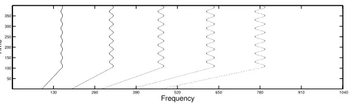
Fig. 1.Ground truth binary map, 1 (black) depicts signal locations and 0 (white) noise locations.

2.1 Ground Truth Conversion

An example of a ground truth binary map is presented in Fig. 1. If no ordered

list of (x, y) coordinates depicting track locations is available the information

needs to be extracted from the binary map prior to calculating the proposed metrics. The modified region grow algorithm presented in Alg. 1 can be used to achieve this. It is assumed that only the centre (strongest) frequency bin for each track is marked and therefore that one frequency bin (for each track) is marked in each time frame.

Initially the algorithm detects a seed point for each track by scanning through the ground truth from top to bottom and left to right. Once a seed point has been found its coordinates are stored as the current point and the track’s next point is searched for. The next row of the ground truth is extracted and if this

contains a track point with a distance less than g from the current point, i.e.

the track has not ended, its coordinates are added to the track list. The current point is updated to the new point’s coordinates and the process is repeated for each row in the ground truth until the track’s end is reached.

The distance thresholdg prevents the end of a traced track being linked to

other tracks in the data. Algorithm 1 has the limitation that it does not account for crossing tracks. If such a condition is needed a hidden Markov model with a state space which accounts for track gradient can be implemented [1].

2.2 Spectrogram Complexity Measure (SCM)

It is assumed that a linear vertical track is much easier to detect than a linear track with unknown gradient which are, in turn, both more simple to detect than a curvilinear or irregular tracks. Also, independent to this, a set of high SNR tracks are much easier to detect than a set of low SNR tracks. Thus, we have the following factors which complicate the detection of tracks within a spectrogram image:

– Signal-to-Noise Ratio (SNR)

– Complexity of tracks

Algorithm 1Convert a binary map into a coordinate list

Input:G, ground truth binary map.

Output:T, an ordered list of coordinates representing each track’s locations.

1: c←0 2: T← ∅

3: form= 1 to height ofGdo{scan for seed point}

4: forn= 1 to width ofGdo

5: if Gn,mis a track pointthen{start grouping track}

6: cp←[n, m]

7: p←m+ 1

8: R←[G1,p,G2,p, . . . ,Gn,p]

9: Find track pointnp= [x, p] inRwhich is closest tocp 10: while(np6=∅)∧(|np−cp|< g)∧(p <height ofG)do

11: PushnpontoTc

12: cp←np

13: p←p+ 1

14: R←[G1,p,G2,p, . . . ,Gn,p]

15: Find track pointnp= [x, p] inGwhich is closest tocp 16: end while

17: Set pixels inGcontained inTcto 0

18: c←c+ 1

19: end if

20: end for

21: end for

22: return T

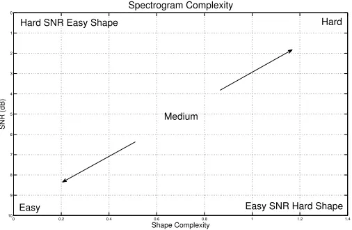
As above, these factors are naturally grouped into two subsets of conditions; SNR related complexity and track shape related complexity. This separation allows for the construction of a two-dimensional plot on which each axis represents one of these factors; the y-axis SNR and the x-axis track complexity. Such a construction is shown in Fig. 2.

We reverse the SNR axis to reflect the increasing difficulty as SNR decreases, in this manner the hardest detection problems (e.g. curvilinear and irregular tracks in low SNR spectrograms) are located in the top right and the easiest (e.g. linear, vertical tracks in high SNR spectrograms) at the bottom left of the distribution and variations are captured between these extremes.

Signal-to-Noise Ratio Complexity After applying Alg. 1 we have an

enu-merated set of coordinate pairsT, through (1), containing the locations of tracks

in a spectrogramS.

T =

C

[

c=1

Tc (1)

An additional set H can be defined which contains all the coordinate pairs

possible inS and therefore N =H\T, contains the noise pixel locations. The

0 0.2 0.4 0.6 0.8 1 1.2 1.4 0 1 2 3 4 5 6 7 8 9 10 Spectrogram Complexity Shape Complexity SNR (dB) Medium Hard SNR Easy Shape

Easy SNR Hard Shape Hard

Easy

Fig. 2.Intended classification boundaries of the proposed distribution.

can then be calculated through (2) and (3).

¯

Pt=

1

|T|

X

t∈T

St₁,t₂ (2)

¯

Pn=

1

|N|

X

n∈N

Sn₁,n₂ (3)

Allowing the SNR ofS, in terms of decibels, to be calculated (4). Which forms

the y-axis of our plot in Fig. 2.

SNR = 10 log10

¯ Pt ¯ Pn (4)

Track Complexity The second metric is also calculated upon the set, T, de-rived with Alg. 1 and is formed to measure the detection complexity of each track within a spectrogram.

As outlined, we propose that the complicating factors in track detection are the track’s gradient and shape. The averaged absolute values of a tracks’ first and second derivatives will form measures of these properties and can be discretely approximated [13] by (5) and (6) (respectively).

δTc

δy ≈

1

|Tc| |Tc|−1

X

y=1

|Tc,y−Tc,(y+1)| (5)

δ2_T c

δy2 ≈

1

|Tc| |Tc|−1

X

y=2

|Tc,(y−1)−2Tc,y+Tc,(y+1)| (6)

where |Tc| is the cardinality of track c and Tc,y is the yth point on track c.

Frequency (Hz)

Time (s)

130 260 390 520 650 780 910 1040

50 100 150 200 250 300 350

Frequency (Hz)

Time (s)

130 260 390 520 650 780 910 1040

50 100 150 200 250 300 350

Frequency (Hz)

Time (s)

130 260 390 520 650 780 910 1040

50 100 150 200 250 300 350

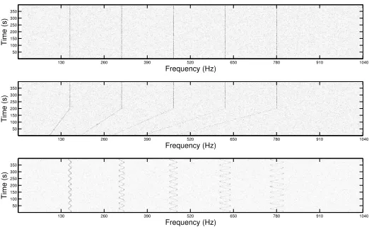
Fig. 3.Examples of spectrograms with varying complexities, giving measure values of: top - 1st

derivative = 0 and 2nd

derivative = 0, middle - 1st

derivative = 0.121 and 2nd derivative = 0.241, and, bottom - 1st

derivative = 0.299 and 2nd

derivative = 0.593.

for a linear sloped track. Whilst the shape measure will be 0 for linear vertical and sloped tracks and positive for a curvilinear and irregular tracks.

The average track measurement within a spectrogram (7) gives a metric which represents a spectrogram’s track complexity.

TC = 1

C

C

X

c=1

δTc

δy + δ2Tc

δy2

(7)

whereCis the number of tracks andTcis thecthtrack present in a spectrogram.

When these measures are used in conjunction with the distribution plot pre-sented in Fig. 2 (with axes representing the SNR and TC), they allow us to visually represent the complexity distribution of a set of spectrograms. With this it is now possible to perform comparisons between algorithms through the comparison of the range of points on the distribution which are within its de-tection capabilities. Importantly, in the absence of a standard test database and without disclosing sensitive datasets, it is possible without testing algorithms on the same dataset. Including this diagram within publications will allow re-searchers to make quick judgements on whether a newly developed algorithm has superior performance and in which areas this occurs. It will also aid researchers in tailoring their test dataset to sufficiently scrutinise an algorithm.

3

Results

Three spectrogram images of varying complexity are presented in Fig. 3. The complexities of these spectrograms, according to the presented metrics, are; top

-0 0.2 0.4 0.6 0.8 1 1.2 1.4 0

1

2

3

4

5

6

7

8

9

10

Track Complexity (S)

SNR (dB)

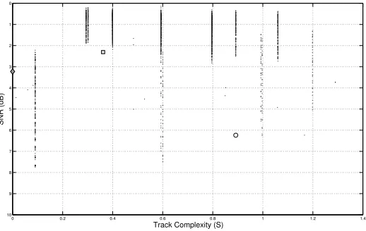
Fig. 4. A SCM distribution, an example of a distribution obtained by applying the proposed measures on a synthetic set of spectrogram images.

SNR = 6.24 dB & TC = 0.892 (for readability sake the SNRs in the plot are not

representative of these figures). The track complexity of the template presented

in Fig. 1 is TC = 0.805, lower than the third spectrogram as it contains a section

of straight sloped track. Figure 4 demonstrates the SCM plot, this example is determined using 2096 synthetic spectrograms. The complexity measurements taken from the spectrograms in Fig. 3 are included (from top to bottom) as diamond, square and circular points. The vertical clustering is due to the data set containing spectrograms with similar track shapes but different SNRs.

Of the three spectrograms, the first contains the easiest track complexity to detect, linear vertical tracks. This is reflected in the measure and, therefore, the distribution plot - the point is located in the far left of the track complexity axis. However, the SNR of this spectrogram is low and therefore the point is located near the top in the SNR axis. The second has a medium track complexity as it exhibits an increase in frequency (linear sloped track) and a similar SNR to the first therefore it is located in a similar area but further to the right in the track complexity axis. And finally, the third represents a more complicated curvilinear track which exhibits high curvature and, therefore, its position in the track complexity axis is towards the far right. Its SNR is relatively high and in this axis it is located below the centre. As desired, the differences of these track shapes are reflected in the proposed measures and distribution plot.

4

Conclusions

in-dicate whether an algorithm which is developed for a specific application will be successful in another. We have achieved this by devising a plot and metrics which express track detection complexity in terms of SNR and track shape.

We have presented some example spectrograms and their complexities ac-cording to our metrics and have included these on a distribution plot derived from a sample data set of synthetic spectrograms with varying track appear-ances and SNRs. It has been shown that the measures successfully separate the differing complexities of each of the spectrograms and that this is reflected in the distribution plot. It is our hope that authors adopt this method to allow the comparison of algorithms without disclosing sensitive datasets and without the availability of a public dataset.

Nota bene _{we have presented measures which determine the difficulty of} de-tecting features contained within a spectrogram image, as such, these measures are independent of the FFT resolution used to derive the spectrogram.

References

1. Xie, X., Evans, R.: Multiple target tracking and multiple frequency line tracking using hidden Markov models. IEEE Trans. on Sig. Proc.39(1991) 2659–2676 2. Lampert, T.A., O’Keefe, S.E.M.: Active contour detection of linear patterns in

spectrogram images. In: Proc. of ICPR’08. (December 2008) 1–4

3. Abel, J.S., Lee, H.J., Lowell, A.P.: An image processing approach to frequency tracking. In: Proc. of the IEEE Int. Conference on Acoustics, Speech and Signal Processing. Volume 2. (March 1992) 561–564

4. Martino, J.C.D., Tabbone, S.: An approach to detect lofar lines. Pattern Recog-nition Letters17(1) (January 1996) 37–46

5. Morrissey, R.P., Ward, J., DiMarzio, N., Jarvis, S., Moretti, D.J.: Passive acoustic detection and localisation of sperm whales (Physeter Macrocephalus) in the tongue of the ocean. Applied Acoustics67(November-December 2006) 1091–1105 6. Mellinger, D.K., Nieukirk, S.L., Matsumoto, H., Heimlich, S.L., Dziak, R.P., Haxel,

J., Fowler, M., Meinig, C., Miller, H.V.: Seasonal occurrence of north atlantic right whale (Eubalaena glacialis) vocalizations at two sites on the scotian shelf. Marine Mammal Science23(October 2007) 856–867

7. Yang, S., Li, Z., Wang, X.: Ship recognition via its radiated sound: The fractal based approaches. J. Acoust. Soc. Am.11(1) (July 2002) 172–177

8. Chen, C.H., Lee, J.D., Lin, M.C.: Classification of underwater signals using neural networks. Tamkang J. of Science and Engineering 3(1) (2000) 31–48

9. Ghosh, J., Turner, K., Beck, S., Deuser, L.: Integration of neural classifiers for passive sonar signals. Control and Dynamic Systems - Advances in Theory and Applications77(1996) 301–338

10. Howell, B.P., Wood, S., Koksal, S.: Passive sonar recognition and analysis using hybrid neural networks. In: Proc. of OCEANS ’03. Volume 4. (September 2003) 1917–1924

11. Shi, Y., Chang, E.: Spectrogram-based formant tracking via particle filters. In: Proc. of IEEE ICASSP. Volume 1. (April 2003) I–168–I–171

12. Duda, R.O., Hart, P.E.: Use of hough transform to detect lines and curves in pictures. Commun. ACM15(1) (Jan 1972) 11–15