Identification of nonlinear time-varying systems using an online sliding-window and common model structure selection (CMSS) approach with applications to EEG

This is a repository copy of

Identification of nonlinear time-varying systems using an online

sliding-window and common model structure selection (CMSS) approach with applications

to EEG

.

White Rose Research Online URL for this paper:

http://eprints.whiterose.ac.uk/74670/

Monograph:

Li, Y., Wei, H.L., Billings, S.A. et al. (1 more author) (2010) Identification of nonlinear

time-varying systems using an online sliding-window and common model structure

selection (CMSS) approach with applications to EEG. Research Report. ACSE Research

Report no. 1019 . Automatic Control and Systems Engineering, University of Sheffield

[email protected] https://eprints.whiterose.ac.uk/ Reuse

Unless indicated otherwise, fulltext items are protected by copyright with all rights reserved. The copyright exception in section 29 of the Copyright, Designs and Patents Act 1988 allows the making of a single copy solely for the purpose of non-commercial research or private study within the limits of fair dealing. The publisher or other rights-holder may allow further reproduction and re-use of this version - refer to the White Rose Research Online record for this item. Where records identify the publisher as the copyright holder, users can verify any specific terms of use on the publisher’s website.

Takedown

If you consider content in White Rose Research Online to be in breach of UK law, please notify us by

Identification of nonlinear time-varying systems using an

online sliding-window and common model structure

selection (CMSS) approach with applications to EEG

Yang Li, Hua-Liang Wei, S. A. Billings, and P. G. Sarrigiannis

Research Report No. 1019

Department of Automatic Control and Systems Engineering The University of Sheffield

Mappin Street, Sheffield, S1 3JD, UK

____________________

*

Identification of nonlinear time-varying systems using an

online sliding-window and common model structure

selection (CMSS) approach with applications to EEG

Yang Li

1

, Hua-Liang Wei

1

, S. A. Billings

1,*

, P. G. Sarrigiannis

2

1

Department of Automatic Control and Systems Engineering,

The University of Sheffield, Mapping Street, S1 3JD, UK

[email protected], [email protected], [email protected],

2

Department of Clinical Neurophysiology, Sheffield Teaching Hospitals NHS

Foundation Trust, Royal Hallamshire Hospital,

Glossop Road, S10 2JF, UK

[email protected]

Abstrac_t—The identification of nonlinear time-varying systems using linear-in-the-parameter models is investigated. A new efficient Common Model Structure Selection (CMSS) algorithm is proposed to select a common model structure. The main idea and key procedure is: First, generate K1 data sets (the first K data sets are used for training, and the



K1



th one is used for testing) using an online sliding window method; then detect significant model terms to form a common model structure which fits over all the

K

training data sets using the new proposed CMSS approach. Finally, estimate and refine the time-varying parameters for the identified common-structured model using a Recursive Least Squares (RLS) parameter estimation method. The new method can effectively detect and adaptively track the transient variation of nonstationary signals. Two examples are presented to illustrate the effectiveness of the new approach including an application to an EEG data set.

I. INTRODUCTION

Many processes in engineering systems and the biomedical field exhibit both time-varying and nonlinear behaviours. The identification of mathematical models of dynamical nonlinear systems is vital in many fields. The procedure of system identification is to construct mathematical models using observed data. The developed mathematical models from neural networks, fuzzy or regressive models can be applied to study the behaviour of the underlying system as well as for supervision, fault detection, prediction, and model-based control. A variety of system identification techniques have been developed for dynamic process modelling. However, the majority of physical and biomedical systems contain complex nonlinear relationships which can include nonlinearities and chaotic behaviour, which are difficult to model with conventional techniques.

During recent years, much attention has been devoted to the problem of identification of time-varying systems. In many practical cases, the system parameters are unknown and are time varying. When the system is given in state-space form, a classical approach consists of applying Kalman filter based algorithms for estimation of time-varying parameters [1]-[4]. The application of the recursive least squares algorithm to the estimation of nonlinear system parameters, often requires the nonlinear model outputs to be expressed linearly in terms of the unknown parameters. A discussion about performance of recursive least squares identification and related adaptive control schemes can be found in [5]-[9]. Neural networks and Markov chain Monte Carlo based identification strategies are also discussed in [10]. Recently, a robust identification and control algorithm with time-varying parameter perturbations has been proposed in [11], where the nonlinear model outputs are expressed linearly in terms of the unknown parameters. Peng et al. [12] introduced parameter estimation methods based on a radial basis functions (RBF) neuronal predictor.

The main contribution of this paper is the introduction of a new Time-Varying Common-Structured (TVCS) modelling scheme as a solution to the time-varying nonlinear systems identification problem, where the selection of the common model structure is the critical step throughout the modelling procedure. A new efficient Common Model Structure Selection (CMSS) algorithm is investigated to select a common model structure using an online sliding window approach. Once the common-structured model has been determined, relevant time-varying model parameters can then be estimated using a RLS algorithm. The novel study of common-structured model identification is particularly useful for engineering system design and control, where only a fixed common model structure is involved but with time-varying parameters. A TVCS model can be used to track fast transient variations of time-varying parameter properties and study the performance of the behaviour of the underlying dynamical systems. The TVCS model is different from the traditional Multi-Input and Multi-Output (MIMO) model structure, where each subsystem model may not need to share the same common model structure and which often involves one single data set. A simulated example and an application to real EEG data are included to demonstrate the performance of the new method.

II. The TIME-VARYING LINEAR-IN-THE-PARAMETER

REGRESSION MODEL

The identification problem of a nonlinear dynamical system is based on the observed input-output data



   



1

, N

t

u t y t _ , where u t

 

and y t

 

are the observations of the system input and output, respectively [18]. This study considers a class of discrete stochastic nonlinear systems which can be represented by the following nonlinear autoregressive with eXogenous inputs (NARX) structure below [19]-[22]:

 





1 ,



,



_y



,



1 ,



,



_u



,



 

y t  f y t y tn u t u tn



e t , (1) where

u t

 

and

y t

 

are the system input and output variables, respectively, n_u and ny

and the observation noise

e t

 

is an uncorrelated zero mean noise sequence providing that the function

f

 

gives a sufficient description of the system. X t

 

 _y t



1 ,



,



_y



,



1 ,



,



_u



T

y tn u t u tn _ denotes the system „input‟ (predictor) vector with a known dimension d n_yn_u, and



is an unknown parameter vector. The NARX model (1) is a special case of the polynomial NARMAX model that takes the form below [23]-[25]

 





























 

1 ,

,

,

1 ,

,

,

1 ,

,

;

y u

e

y t

f y t

y t

n

u t

u t

n

e t

e t

n



e t

















, (2)

The NARMAX model (2) was developed and discussed in [13]-[14].

The non-linear mapping f

 

of (1) can be constructed using a class of local or global basis functions including radial basis functions (RBF), kernel functions, neural networks, multiresolution wavelet such as B-splines and different types of polynomials such as the Chebyshev and Legendre types [13], [26]-[36]. The polynomial model representation of a nonlinear time-varying NARX is represented below

 

   

     

 

   

1 1 1 2 1 2

1 1 2 1

1 1 1 0 , 1 1 d k d d

d d d

i i i i i i

i i i i

d d d

i i i

i i i k

y t t x t t x t x t

t x t e t









          





 



, (3)

where



₀ is a constant term, and

 

1, d i i

t



are time-varying parameters and

 

_



_



_

_

1

1

y k

y y

y t

k

k

n

x t

u t

k n

n

k

d



 



 





  



, (4)

The degree of a multivariate polynomial is defined as the highest order amongst the terms. If the number of regressors is m and the maximum polynomial degree is



, the number of parameters (number of polynomial terms) is

 





! ! ! t d n d 







 , (5)

For large lags n and y n , the regression model (1) often involves a large number of u

candidate model terms, even if the nonlinear degree  is not very high. For example, if

10

candidate model with a large number of candidate model terms can often be drastically reduced by including in the final model only the effectively selected significant model terms. The main motivation of the present study is to select significant common-structured model terms to form a parsimonious common model structure which generalises well [37].

The polynomial NARX model of time-varying linear-in-the-parameter can now be formulated as [38]

 

     

     

1 M

T m m

m

y t



t



t e t



t t e t







    , (6)

where

M

is the total number of candidate regressors. _m

 

t _m



X t

 





m1, ,M



are nonlinear functions (they do not contain parameters) and m

 

t



m1, ,M



represents the

model time-varying parameters. 

 

t  ₁



X t

 



, ,_M



X t

 



_T and 

 

t are the

associated regressor and parameter vectors, respectively. It is should be noted that in most cases the initial full regression Eq. (6) might be highly redundant. Some of the regressors or model terms can be removed from the initial regression equation without any effect on the predictive capability of the model, and this elimination of the redundant regressors usually improves the model performance [39]-[40]. For most nonlinear dynamical system identification problems, only a relatively small number of model terms are commonly required in the regression model. Thus an efficient model term selection algorithm is highly desirable to detect and select the most significant regressors.

III.

TVCS MODEL IDENTIFICATION

The CMSS algorithm is a critical step in TVCS identification. Once the common-structured model has been identified, relevant model parameters for each data set can then be estimated, and the transient properties of the model parameters on the associated data set can thus be deduced. The identification procedure for TVCS models contains the following steps:

Step 1) Data acquisition. For an original N-sample observational input-output data

   



,



N₁

N _t

sliding window of length W, with 50% overlap, where the parameter K1

is equal to _N/



W/ 2



_1, and  _{ }x denotes taking the upper integer part of the variable x. Note that the window of length

W

was chosen to satisfy the recommended minimum sample size determination discussed in [41].

Step 2) CMSS algorithm. This will be described in detail in section § B below.

Step 3) Model parameter estimation. The parameters for the TIVCS model can be easily calculated using Eq. (25). The parameters for the TVCS model can be estimated using a recursive algorithm for each data window of the



K1



th data sets. The transient properties of the observational data can thus be deduced by the transient parameter values for the associated data set.

A.

The multiple regression model

Assume that a total of



K1



data sets (where the first K represent the training data sets, and the last data set is used as a test data set) obtained by the online sliding window have been carried out on the same system. Also, assume that a common model structure of Eq. (6) can be best fit to all the training data sets. Denote the observed input-output sequences for the

k

th data set by



   



1

, k

k

N

N k k _t

D  u t y t _ for k1,2, ,K1. Thus the

k

th „input‟ (predictor) vector is represented by X t_k

 

 x_k,1

 

t , ,x_{k d,}

 

t _T _y t_k



1 ,



,y t_k



n_y



,



1 ,



,





T

k k u

u t u tn  . Assume that all the

K

data sets can be represented using a common model structure for the different parameters, then the initial candidate multiple regression model can be formulated as [25]

 

,



 



 

, ,

 

 

1 1

M M

k k m m k k k m k m k

m m

y t

 

X t e t

 

t e t

 





 



 , (7)

where the parameters



_{k m,} in Eq. (7) are time-independent constants, Eq. (7) will be called the time-invariant common structure (TIVCS) model. If the parameters



k m, are

time-dependent, the time-varying common structure (TVCS) model is represented by

 

,

 



 



 

,

 

,

 

 

1 1

M M

k k m m k k k m k m k

m m

y t



t



X t e t



t



t e t

 

where _{k m,}

 

t _m



X t_k

 



for k1, 2, ,K , m1,2, ,M , and t1, 2, ,N_k . The representation of Eq. (8) using a compact matrix form can be expressed as

k k k k

      , (9) where   _{k }y_k

 

1 , ,y N_k

 

_k _T,   _k _k,1

 

t , ,_{k M,}

 

t _T,   _{k }e_k

 

1 , ,e_k

 

N_k _T, and

  

_k





_k,1

,

,



_{k M,}



_

with , ,

 

1 , , ,

 

T k m k m k m Nk



_{ }





_ for k1, 2, ,K and 1, 2, ,

m M.

B.

The common model structure selection (CMSS) algorithm

In this subsection, a new CMSS algorithm, which can be regarded as an extension of the orthogonal forward regression (EOFR) algorithms ([14], [42]) will be developed to select a common-structured sparse model from the multiple regression shown in Eq. (7) and (8). Let



1, 2, ,



I M , and denote D



m:mI



as the dictionary of candidate model terms for an initially chosen candidate common model structure which fits to all the

K

regression models given by Eq. (7) and (8). For the

k

th data set, the dictionary D can be used to form a dual dictionary  _k



_{k m,} :m I



, note that the m th candidate basis vector _{k m,} is formed by the m th candidate model term _mD , namely,

 



 







, 1 , ,

T

k m m Xk m Xk Nk

 _{ }  

 for k1, 2, ,K . Thus the CMSS problem is equivalent to finding a subset





1, 2, , n

p p p D

    (normally n M ) from the dictionary



m:



D  mI . So that _k



k1, 2, ,K



can be approximated using a linear combination of regression terms





1

, , , , n

k p k p k

    below

 

₁

 

,1 , , , n

k



k

t



k p



k n

t



k p k

 

 



, (10) The CMSS algorithm selects significant model terms in a forward stepwise way, one model term at each search step. Let rk,0  k for



k1, 2, ,K



. For k1, 2, ,K, and

1,2, ,

 

_{ }











2 , 1 , ,

,

T k k i

T T

k k k i k i

err

k i



 





 

, (11)

and define

 1

_{ }

1

1

1

1

arg max

,

K i M

k

p

err

k i

K

  _







_

_







, (12)

Note that

err

 1

 

k i

,

in Eq. (11) can be explained as the error reduction ratio (ERR) that is introduced by including the mth basis vector _{, ,}

m k m k p







into the

k

th regression model, a detailed description of ERR can be seen Chen et al., [13] and Billings et al., [43]. The first significant common model term can be selected as the p₁th element,

1 p D



 from Eq. (11) and (12). Thus the first significant basis vector for the

k

th regression model is

1 ,1 , k k p







,

and the associated orthogonal basis vector can be chosen as

1 ,1 , k k p

q 



. For the first step search, the model residual for the

k

th regression model is defined by

,1 ,1 ,0

,1 ,1 T k k

k k T

k k

q

r

r

q q







, (13)

Generally, the mth significant model term of

k

th regression model



k p, _m can be chosen by

the following steps. It is assumed that at the



m



1



th step,



m



1



significant model terms, namely,





_k,1

,

,



_{k m, 1}



, have been selected. Let





_k,1

,

,



_{k m, 1}



be the associated basis vectors for the

k

th regression model, and assume that the



m



1



selected bases have been transformed into a new group of orthogonal bases



q

_k,1

,

,

q

_{k m, 1}



via a modified Gram-Schmidt orthogonal transformation. Let

  1 , ,

, , ,

1 , ,

,

,

T m

m k j k p

k i k i T k p m p k p k p

q

s

q

i

J

q

q

















(14)

where

J

_m





i

:1

 

i

M i

,



p

_t

,1

  

t

m

1



, for k1, 2, ,K and iJ_m, calculate

 

_{ }



 









 

   



, , , , , T m T k k i m

T m m T

k k k i k i

s err k i

s s

 

and define

 

_{ }

1

1

1

arg max

,

K m m

i M k

p

err

k i

K

  _







_

_







, (16)

Similar to

err

 1

 

k i

,

defined by Eq. (11), the

err

 m

 

k i

,

given by Eq. (15) is an indicator which shows the correlation dependence of _k on

s

 _{k i}m_, , and the most significant common vectors can be determined by maximising (16). The mth significant common model term can then be chosen as the p_mth element,

m p D



 . Thus the mth significant basis vector for the

k

th regression model is



k m, 



k p, _m, and the associated orthogonal

basis vector can be selected as _,  _,

m m k m k p

q



s

. For the mth step search, the model residual for the

k

th regression model is formulated as

,

, , 1 ,

, , T k k m k m k m T k m

k m k m

q

r

r

q

q

q









, (17)

Similarly

err

 1



k p

,

₁



given by Eq. (11), the

err

 m



k p

,

_m



can be explained as the error reduction ratio (ERR) that is introduced by including the mth basis vector _{, ,}

m k m k p







into the

k

th regression model. By maximising the sum of the ERR values for all the K data sets, the criterion (16) guarantees that the variation of the outputs in all the K data sets can be explained by including the model term

m p



, with the highest percentage, compared with choosing any other candidate model term



D. The quantity

 

_

_

1 1 , K m m k

AERR err k p

K 





, (18)

is referred to as the mth average error reduction ratio (AERR). The criterion (18) provides a way to select significant vectors one by one. Once the first



m1



basis vectors





k,1

,

,



k m, 1



have been determined, and the associate orthogonal vectors



q

k,1

,

,

q

k m, 1



can be obtained, then these



m



1



vectors together with the mth vector

, , m k m k p







, and the associated orthogonal vector _,  _,

m m k m k p

the outputs of the

K

datasets with a higher percentage, compared with any other candidate vectors. This step-by-step forward selection algorithm is a non-exhaustive search approach, which usually produces satisfactory and nearly optimal results, see for example [25], [38]. From Eq. (17), the vectors r_{k m,} and q_{k m,} are orthogonal, then





2

2 2 ,

, , 1

, , T k k m k m k m T

k m k m

q

r

r

q

q









, (19) by respectively summing Eq. (18) and (19) for m from 1 to n(generally

n

M

), yields

,

, , 1 , ,

T n

k k m

k T k m k n m k m k m

q

q

r

q

q





 





, (20)





2





2

2 2 , 2 ,

, , 1

1

, , , ,

T _n T

k k n k k m

k n k n T k T

m

k n k n k m k m

q

q

r

r

q q

q

q













 





, (21)

From Eq. (20) and (21), the model residual rk n, can be used to form a criterion for model

term selection, and the search procedure will be terminated at the nth step if the norm

2 , k n

r 



, (22) is satisfied. This produces a parsimonious model containing n regressors.

An appropriate value for



is problem dependent and must be learned empirically. Alternatively, the generalized cross-validation (GCV) criterion [28] can be adopted to terminate the CMSS procedure. Specially, for the

l

-term model, the GCV of single regression model is defined as

 

N 2 ( ) N 2 rl 2

GCV l MSE l

N



l N



l N

   

_{ } _{ }

 

    , (23)

where





max 1, N







and 0 



0.01. As a rule of thumb, it was suggested [44] that a good choice for



is to use a value from the range of 5  10. The average GCV (AGCV) is formulated by

 

 

_{ }

1

1 K

k k

AGCV l GCV l

K 





, (24)

n-term model. Instead of using the MSE criterion (21), other criteria including Approximate Minimum Description Length (AMDL) [45], Bayesian information criteria (BIC) [46]-[48] can also be adopted for the CMSS procedure.

C.

Parameter estimation

For the TIVCS model (7), it is easy to verify that the relationship between the selected

bases





1

, , , , n

k p k p k

    and the associated orthogonal bases



q

_k,1

,

,

q

_{k n,}



, for the

k

th data set, is shown as

, , , k n k n k n

A Q R , (25) where _{, 1}

,

,

_,

n k k p k p

A

 









_

, Q_{k n,} is an N_kn matrix with orthogonal columns q_k,1,

,2, , , k k n

q q , and Rk n, is an n n unit upper triangular matrix whose entries are calculated

during the orthogonalisation procedure. The unknown time-invariant parameter vector in Eq. (7), denoted by



_{k n,}  



_k,1, ,



_{k n,} _T, for the regression with respect to the original vectors, can be calculated from the triangular equation Rk n,



k n, Lk n, with , ,1, , ,

T k n k k n

L  L L _ , where

L

_m





r

_{k m}T_{, 1}

q

_{k m,}

 

/

q

_{k m k m}T_,

q

_,



for m1, 2, ,n.

For TVCS model of Eq. (8), it is also easy to calculate the value of the unknown time-dependent parameters by recursive least squares. For the

k

th sliding window data set, the estimation of



_{k n,}

 

t

in Eq. (8) can be obtained by

 





 



 

  





, , , , , ,

ˆ ˆ ₁ T ˆ ₁

k n t k n t gk n t yk n t k n t k n t







  





 , (26) where

 

   



  



 



  



1

, , , , 1 , , , 1 ,

T

k n k n k n k n k n k n k n k n

g t P t



t P t



t

 

 t P t



t  , (27) and

 



   







, , , ,

1

1

T

k n k n k n k n

P

t

I

g

t



t

P

t



IV. CASE STUDY

Two examples are provided to illustrate the applicability and effectiveness of the proposed TVCS model identification procedure. The data used in the first example are simulated from a nonstationary model. The objective is to illustrate that the effectiveness of the novel TVCS model approach to deal with severely nonstationary processes. The second example involves a real-world modelling problem of EEG data.

A.

Example 1: Simulation data

Prior to applying the proposed TVCS modelling approach to real EEG data, an artificial time-varying signal was considered. The signal below was simulated

 

7



0



1

cos 2

i i

i

y t A



f t









 , (29)

where 1, , , , ,1 1 1 1 1,1 , 3 5 7 9 11 13

A  _

  f 



50,150, 250,350, 450, 600, 750 ,



initial phase shift 0

3 2



  ,

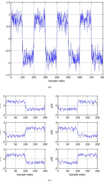
and sample timet is 0.08 second, respectively. The above signal was sampled with a sampling interval 0.0001, and thus a total of 800 observations shown in Figure 1(a) were obtained. A Gaussian white noise sequence, with mean zero and variance of 0.04, was then added to the 800 data points.

The objective is to identify a TVCS model, and then the transient dynamical properties of the analytical signal can be deduced from the time-varying parameters. Denote the system output sequences using

 

 

1 N

t

y t

 , with N = 800. The online sliding window of length W =

200 is applied to obtain the KN/



W/ 2



1= 7 data sets. Here from the properties of the simulation signal the sliding window length should be chosen as

W

= 200, with 50% overlap. Six training data sets numbered y01 to y06 shown in Figure 1(b) were used for the common-structured model identification, and the 7th data set was used to test the performance of the identified model. The predictor vector for all the common-structured models was chosen to be X t

 

 _x t₁

 

, ,x t₅

 

_T, where x tk

 

y t



k



for k1, ,5. The initial

 

0 5

 

5 5 ,

     

1 1

i i i j i j

i i j i

y t





x t



x t x t e t

  

 







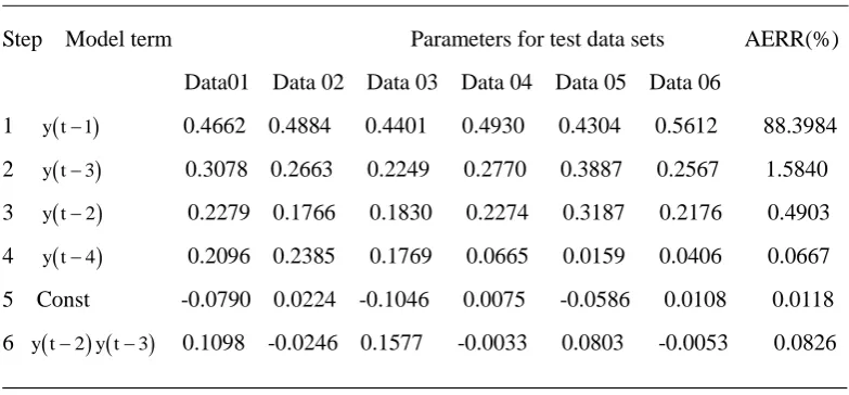
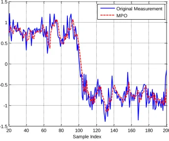
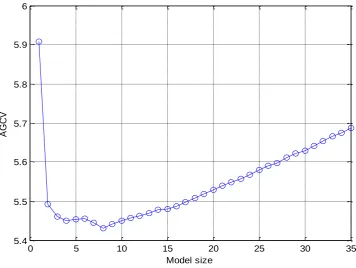
 , (30)

This candidate model involves a total of 21 candidate model terms from Eq. (5). Based on the candidate common model structure, the novel CMSS algorithm was applied to the six training data sets. The AGCV criterion, shown in Figure 2, suggests that a common model structure, with sixmodel terms, is preferred. The six selected common model terms, ranked in order of significance are shown in Table 1. Now consider the performance of the identified model, whose parameters are determined by Eq. (25) and Table 1. The 7th test data set, which has never been used in the identification procedure, was applied to test the performance of the identified model. Figure 3presents a comparison between the Model Predicted Output (MPO) and the original measurements. Note that the MPO is defined as

 

ˆ













ˆ ˆ 1 , ,ˆ 5

y t  f y t y t , implying that y t is produced from the identified model ˆ

 

iteratively. Note that the model predicted output (MPO) can reveal severe model deficiencies which would otherwise go undetected by one-step-ahead predictions.

To quantitatively measure the identified models, the normalized root mean squared error (RMSE) is defined as follows:

   

 

1

2 2 1

1

ˆ

1 NK t K

y t y t RMSE

N _{y t}



 







, (31)

where N_K1 is the data sliding window length of the



K1



th test data set, y t is the ˆ

 

predicted value from the identified model. The RMSE criteria in Eq. (31) can also be provided to select a proper sliding window of length

W

provided that the RMSE value is very small. The value for RMSE, for the identified models, over the test data set, was calculated as RMSE = 2.2051%. Clearly the identified model provides an excellent presentation for the test data set.

The TVCS model was thus represented by

 

0

 

4

  



5

  

 

  

1

2 3

i i

y t



t



t y t i



t y t y t e t



 



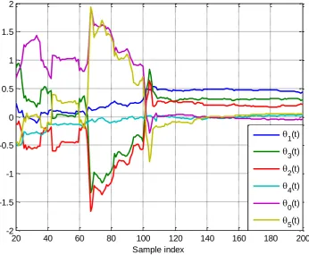
     , (32)

parameters can be directly estimated using the RLS algorithm. Figure 4 shows the estimated values for



 

t

for the test data set given in Figure 3 using the RLS algorithm with a forgetting factor of 0.98.The time-varying coefficients estimates in Figure 4 can give more transient information, for example, there are two clear abrupt changes of the estimated coefficients at sample index interval from 60 to 80, and from 100 to 120, respectively, which show that the original signal shown in Figure 3 undergoes transient changes. Furthermore, the proposed method can also track variation of each training data block dynamically, for example, Figure 5(b) shows the rapid change of coefficient estimation at about sample index 100, which implies that the original training data block changed at about sample index 100. The results discussed above are show that the CMSS algorithm is effective.

B.

Example 2: modelling EEG Data

Scalp EEG signals are synchronous discharges from cerebral neurons detected by electrodes attached to the scalp. The EEG signals discussed here were recorded with the same 32-channel amplifier system. An XLTEK 32 channel headbox (Excel-Tech Ltd) with the international 10-20 electrode placement system was used in the Sheffield Teaching Hospitals NHS Foundation Trust, Royal Hallamshire Hospital, UK. The sampling frequency of the device was 500 Hz. Symmetrical two channels (F3, located over the left superior frontal area

Step Model term Parameters for test data sets AERR(%)

Data01 Data 02 Data 03 Data 04 Data 05 Data 06

1 y t 1 0.4662 0.4884 0.4401 0.4930 0.4304 0.5612 88.3984

2 y t 3 0.3078 0.2663 0.2249 0.2770 0.3887 0.2567 1.5840

3 y t 2 0.2279 0.1766 0.1830 0.2274 0.3187 0.2176 0.4903

4 y t 4 0.2096 0.2385 0.1769 0.0665 0.0159 0.0406 0.0667

5 Const -0.0790 0.0224 -0.1046 0.0075 -0.0586 0.0108 0.0118

6 y t 2 y t3 0.1098 -0.0246 0.1577 -0.0033 0.0803 -0.0053 0.0826

[image:16.595.96.488.379.561.2]

Table 1 Identification results for the simulation data with the CMSS algorithm for NAR model representation

of the brain and F4, located over the same area on the right) of EEG recorded from a patient with absence seizure epileptic discharge is investigated in this example, where Channel F3 is the signal input and Channel F4 is the signal output, the main reason is that the phase of Channel F4 is related to the phase of channel F3. The input-output EEG signals of N = 3000 data points pairs of one seizure, which are for a sort of epileptic seizure activity of a patient, with a sampling rate of 500 Hz, recording during 6 seconds, were obtained.

Similar to the previous simulation example, the objective is to identify a TVCS model which can be used to analyse transient properties of EEG signals and dynamically track the variation of the EEG signals using an online sliding window approach. Simulation results have shown that, the choice of sliding window of length W = 600 data points, gives good model identified results. So the parameter

K

was set to equal to 9. The first 8 datasets will be considered as training data sets, shown in Figure 6, for the model identification, and the 9th test data set which has never been used in the identification procedure was then used to test the performance of the identified model. Denote the system input and output sequence using

   



,



N₁

N _t

D  u t y t _ with N = 3000 data pairs. The predictor vector for all the common-structured models was chosen to beX t

 

 _x t₁

 

, ,x₁₀

 

t _T, where x tk

 

 y t



k



for k1,2, ,5 and x tk

  

u t k 5



for k6,7, ,10. The initial candidate common model structure for all the 8 training data sets was chosen to be a NARX model below

 

0 10 10 10 ,

     

1 1

i i j i j i i j i

y t







x t x t e t

  

 

 

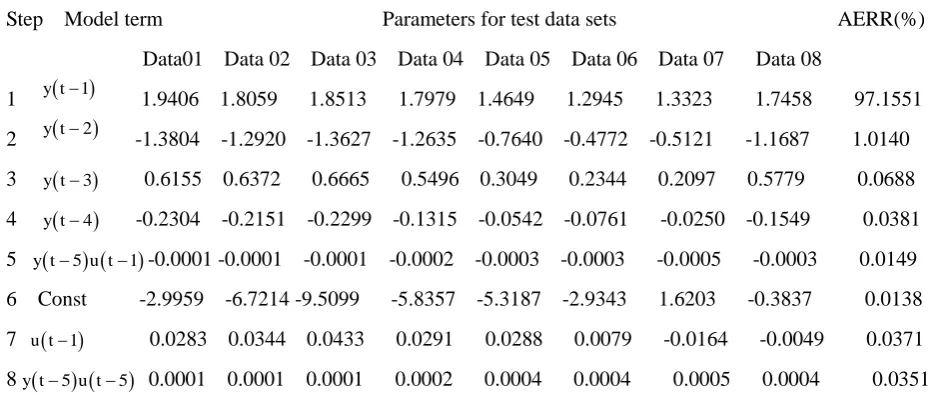
  , (33)

This candidate model involves a total of 66 candidate model terms. Based on the candidate common model structure, the new CMSS algorithm was applied to the 8 training data sets. The AGCV index, shown in Figure 7, suggests that a common model structure, with 8 model terms is preferred. The 8 selected common model terms, ranked in order of the significance, are shown in Table 2. The TIVCS model for the 8 training data sets was represented by

 

 







 





 

  

4

0 5

1

6 7

1

5

1

5

5

i i

y t

y t

i

u t

y t

u t

y t

u t

e t

















 







 



 



, (34)

test data set. The output from the model (34) was then compared with the corresponding measurements. Figure 8 shows a comparison between the model output and the associated measurements. The normalized root-mean-square-error (RMSE), with respect to the test data set, was calculated to RMSE = 0.2755%. Clearly, the TIVCS model provides an excellent representation for the test data set.

where RMSE is 0.2755%.

Thus the TVCS model can be represented by

 

 

   

  



  

 



  

 

  

4

0 5

1

6 7

1

5

1

5

5

i i

y t

t

t y t

i

t u t

t y t

u t

t y t

u t

e t

















 







 



 



, (35)

where the parameter



 

t

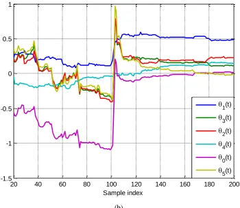
is time-dependent. The time-varying parameters can directly be estimated using the RLS algorithm. In Figure 9, the estimated values for 

 

t , corresponding to the original test data block given in Figure 8, using the RLS algorithm with a forgetting factor of 0.98, are shown and reveal the abrupt changes of coefficient estimation which takes place at sample index from 100 to 150, and about 450, respectively. These estimation results reveal the transient information in the original EEG data block. Similar to the previous

Step Model term Parameters for test data sets AERR(%)

Data01 Data 02 Data 03 Data 04 Data 05 Data 06 Data 07 Data 08

1 y t 1 1.9406 1.8059 1.8513 1.7979 1.4649 1.2945 1.3323 1.7458 97.1551

2 y t 2 -1.3804 -1.2920 -1.3627 -1.2635 -0.7640 -0.4772 -0.5121 -1.1687 1.0140

3 y t 3 0.6155 0.6372 0.6665 0.5496 0.3049 0.2344 0.2097 0.5779 0.0688

4 y t 4 -0.2304 -0.2151 -0.2299 -0.1315 -0.0542 -0.0761 -0.0250 -0.1549 0.0381

5 y t 5 u t1-0.0001 -0.0001 -0.0001 -0.0002 -0.0003 -0.0003 -0.0005 -0.0003 0.0149

6 Const -2.9959 -6.7214 -9.5099 -5.8357 -5.3187 -2.9343 1.6203 -0.3837 0.0138

7 u t 1 0.0283 0.0344 0.0433 0.0291 0.0288 0.0079 -0.0164 -0.0049 0.0371

8y t 5 u t5 0.0001 0.0001 0.0001 0.0002 0.0004 0.0004 0.0005 0.0004 0.0351

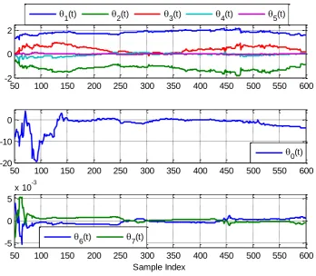
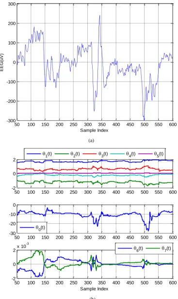
[image:18.595.85.551.247.457.2]

example 1 discussed above, the proposed method can also be applied to track the variation of EEG data dynamically. For example, in Figure 10(a), the time-varying coefficients are estimated using a RLS algorithm with a forgetting factor of 0.98, corresponding to the EEG training data block „output 2‟ given in Figure 10(a), where the estimation results clearly reveal that abrupt changes have taken place at sample index from 300 to 350, and about 500, respectively. These estimated results above can be applied for feature extraction and classification of EEG data which will be discussed in later publications.

V.

CONCLUSIONS

The application of the new common model structure selection (CMSS) approach involves two critical steps: model term selection and model parameter estimation. When the CMSS algorithm is applied in model structure selection, a multiple regression search procedure, over a number of partitioned data sets, is performed. Initially the implementation of a multiple search appears to be very complex. But the introduction of the new multiple orthogonal regression search algorithm provides an attractive solution to this problem. It should be noted that the computational complexity of the CMSS algorithm depends on the K data sets, where the parameter K depends on the sampled data length N and the sliding window of length W (KN/



W/ 2



1). The choice of the sliding window of length W depends on the properties of the observational data. The true model structure of the underlying system will in many cases be unknown and only the input and output observations are available. But the algorithms derived in this study show that a common model structure can be deduced from the available observations. In the two examples, polynomial models were employed to form the common-structured models. However, it should be noted that the CMSS approach can also be applied to any other parametric or non-parametric modelling problems where the initial full models can be written as a linear-in-the-parameters representation.

this study at this stage is focused on parametric modelling, which forms the basis of some important developments for further application in medical applications including EEG data modelling, analysis, and feature extraction. For example, the time-varying parameter results estimated from the TVCS model can not only provide the transient local information of the EEG signals, but can also be applied in nonlinear time-dependent parametric spectral analysis in the frequency domain to extract more features from EEG signals, so that the results can be further applied for EEG data feature extraction, classification and diagnostic tasks. This work will be reported future studies.

ACKNOWLEDGEMENTS

Yang Li acknowledges the support provided by the University of Sheffield under the scholarship scheme and the authors gratefully acknowledge that this work was supported by the Engineering and Physical Sciences Research Council (EPSRC), UK and the European Research Council (ERC).

REFERENCES

[1] L. Guo, “Estimating time-varying parameters by the Kalman filter based algorithm: Stability and convergence,” IEEE Trans. Automatic Control, vol. 35, no. 2, pp. 141-147, Feb. 1990.

[2] M. Niedzwiecki, “Identification of time-varying systems with abrupt parameter changes,” Automatica, vol. 30,

no. 3, pp. 447-459, Mar. 1994.

[3] M. Niedzwiecki, and W. A. Sethares, “Smoothing of discontinuous signals-the competitive approach,” IEEE

Trans. Signal Processing, vol. 43, no. 1, pp. 1-13, Jan, 1995.

[4] M. Niedzwiecki, “Optimal and suboptimal smoothing algorithm for identification of time-varying systems with randomly drifting parameters,” Automatica, vol. 44, no. 7, pp. 1718-1727, Jul. 2008.

[5] M. C. Campi, “Exponentially weighted least squares identification of time-varying systems with white disturbances,” IEEE Trans. Signal Processing, vol. 42, no. 11, pp. 2906-2914, Nov. 1994.

[6] R. S. S. Pena, and C. G. Galarza, “Practical issues in robust identification,” IEEE Trans. Control Systems

Technology, vol. 2, no. 1, pp. 54-56, Mar. 1994.

[7] A. E. Nordsjo, and L. H. Zetterberg, “Identification of certain time-varying nonlinear Wiener and hammerstein systems,” IEEE Trans. Signal Processing, vol. 49, no. 3, pp. 577-592, Mar. 2001.

[8] M. Niedzwiecki, and T. Klaput, “Fast recursive basis function estimators for identification of time-varying processes,” IEEE Trans. on Signal Processing, vol. 50, no. 8, pp. 1925-1934, Aug. 2002.

[9] M. Niedzwiecki, and T. Klaput, “Fast algorithms for identification of periodically varying systems,” IEEE

Trans. on Signal Processing, vol. 51, no. 12, pp. 3270-3279, Dec. 2003.

of Systems Architecture, vol. 47, no. 7, pp. 587-599, Jul. 2001.

[11]T. A. Ahmed, F. Floret, and F. L. Lamnabhi, “Robust identification and control with time-varying parameters perturbations,” Mathematical and Computer Modelling of Dynamical Systems, vol. 10, no. 3-4, pp. 201-215, Sep. 2004.

[12]H. Peng, T. Ozaki, O. V. Haggan, Y. Toyoda, “A parameter optimization method for radial basis function type models,” IEEE Trans. on Neural Networks, vol. 14, no.2, pp. 432-438, Mar. 2003.

[13]S. Chen, S. A. Billings, C. F. N. Cowan, and P. M. Grant, “Practical identification of NARMAX models using

radial basis functions,” International Journal of Control, vol. 52, no. 6, pp. 1327-1350, Dec. 1990.

[14]S. Chen, and S. A. Billings, “Representation of non-linear systems: The NARMAX model,” International

Journal of Control, vol. 49, no. 3, pp. 1013-1032, Mar. 1989.

[15]J. G. Kuschewski, S. Hui, S. H. Zak, “Application of feedforward neural networks to dynamical system identification and control,” IEEE Trans. Control Systems Technology, vol. 1, no. 1, pp. 37-47, 1993.

[16]R. J. Schilling, J. J. Carroll, A. Ajlouni, “Approximation of nonlinear systems with radial basis function neural networks,” IEEE Trans. Neural Networks, vol. 12, no. 1, pp. 1-15, 2001.

[17]G. Kenne, A. T. Ahmed, L. F. Lamnabhi, H. Nkwawo, “Nonlinear systems parameters estimation using radial basis function network” Control Engineering Practice, vol. 14, no. 7, pp. 819-832, Jul. 2006.

[18]I. J. Leontaritis, and S. A. Billings, “Experimental-Design and Identifiability for Nonlinear-Systems,”

International Journal of System Science, vol. 18, no. 1, pp. 189-202, Jan. 1987.

[19]I. J. Leontaritis, and S. A. Billings, “Input-Output Parametric Models for Non-linear Systems, part I:

Deterministic Non-linear Systems,” International Journal of Control, vol. 41, no. 2, pp. 303-328, Feb. 1985.

[20]L. Ljung, “Black-box models from input-output measurements,” in proceedings of 18th IEEE Instrumentation

and Measurement Technology Conference (IMTC2001), vol. 1, pp.138-146, Budapest, Hungary, May 21-23,

2001.

[21]H. L. Wei, S. A. Billings, and J. Liu, “Terms and Variable Selection for nonlinear system identification,”

International Journal of Control, vol. 77, no. 1, pp. 86-110, Jan. 2004.

[22]S. Chen, X. X. Wang, and C. J. Harris, “NARX-Based Nonlinear System Identification Using Orthogonal Least Squares Basis Hunting,” IEEE Trans. On Control Systems Technology, vol. 16, no. 1, Jan. 2008. [23]S. Chen, S. A., Billings, and W. Luo, “Orthogonal least squares methods and their application to non-linear

system identification,” International Journal of Control, vol. 50, no. 5, pp. 1873-1896, Nov. 1989.

[24]J. Sjoberg, Q. Zhang, L. Ljung, A. Benveniste, B. Delyon, P. Glorennec, H. Hjalmarsson, and A. Juditsky, “Nonlinear black-box modelling in system identification: A unified overview,” Automatica, vol. 31, no. 12, pp. 1691-1724, Dec. 1995.

[25]H. L. Wei, and S. A. Billings, “Improved model identification for non-linear systems using a random subsampling and multifold modelling (RSMM) approach,” International Journal of Control, vol. 82, no. 1, pp. 27-42, Jan. 2009.

[26]S. A. Billings, and H. L. Wei, “The wavelet-NARMAX representation: a hybrid model multiresolution wavelet decompositions,” International Journal of Systems Science, vol. 36, no. 3, pp. 137-152, Feb. 2005. [27]S. A. Billings, and H. L. Wei, “Sparse model identification using a forward orthogonal regression algorithm

aided by mutual information,” IEEE Trans. on Neural Networks, vol. 18, no. 1, pp. 306-310, Jan. 2007.

[28]S. A. Billings, H. L. Wei, and M. A. Balikhin, “Generalized multiscale radial basis function networks,” Neural

Networks, vol. 20, no. 10, pp. 1081-1094, Dec. 2007.

[29]C. J. Harris, X. Hong, and Q. Gan, Adaptive Modelling, Estimation and Fusion from Data: A neurofuzzy

Approach, Berlin: Springer-Verlag, 2002.

[31]Y. Li, H. L. Wei, and S. A. Billings, “Identification of Time-Varying Systems Using Multi-Wavelet Basis Functions,” IEEE Trans. on Control Systems Technology, in press.

[32]K. H. Chon, H. Zhao, R. Zou, and K. Ju, “Multiple time-varying dynamic analysis using multiple sets of basis functions,” IEEE Trans. on Biomedical Engineering, vol. 52, no. 5, pp. 956-960, May, 2005.

[33]M. Niedzwiecki, “Fuctional series modelling approach to identification of nonstationary stochastic systems,”

IEEE Trans. Automatic Control, vol. 33, no. 10, pp. 955-961, Oct. 1988.

[34]M. Niedzwiecki, Identification of Time-Varying Process, New York: Wiley, 2000.

[35]M. Niedzwiecki, and P. Kaczmarek, “Identification of Quasi-Periodically Varying Systems Using the Combined Nonparametric/Parametric Approach,” IEEE Trans. on Signal Processing, vol. 53, no. 12, pp. 4588-4598, Dec. 2005.

[36]R. B. Pachori, and P. Sircar, “EEG signal analysis using FB expansion and second-order linear TVAR process,” Signal Processing, vol. 88, no. 2, pp. 415-420, Feb. 2008.

[37]L. A. Aguirre, and S. A. Billings, “Dynamical effects of overparametrization in nonlinear models,” Physica D,

vol. 80, no. 1-2, pp. 26-40, Jan. 1995.

[38]H. L. Wei Z. Q. Lang and S. A. Billings “Constructing an overall dynamical model for a system with

changing design parameter properties,” Int. J. Modelling, Identification and Control, vol. 5, no. 2, pp. 93-104,

2008.

[39]L. A. Aguirre, and S. A. Billings, “Validating identified nonlinear models with chaotic dynamics,”

International Journal of Bifurcation and Chaos, vol. 4, no. 1, pp. 109-125, Feb. 1994.

[40]S. A. Billings, and Q. M. Zhu, “Validation tests for multivariable nonlinear models including neural networks,” International Journal of Control, vol. 62, no. 4, pp. 749-766, Oct. 1995.

[41]D. H. Hwang, W. A. Schmitt, G. Stephanopoulos, and G. Stephanopoulos, “Determination of minimum sample size and discriminatory expression patterns in microarray data,” Bioinformatics, vol. 18, no. 9, pp. 1184-1193, Sep. 2002.

[42]M. Korenberg, S. A. Billings, Y. P. Liu, and P. J. Mcllroy, “Orthogonal parameter estimation algorithm for

non-linear stochastic systems,” International Journal of Control, vol. 48, no. 1, pp. 193-210, Jul. 1988.

[43]S. A. Billings, S. Chen, and R. J. Backhouse, “The Identification of Linear and Non-linear Models of a Turbo

Charged Diesel-Engine,” Mechanical Systems and Signal Processing, vol. 3, no. 2, pp. 123-142, Apr. 1989.

[44]S. A. Billings, and H. L. Wei, “An adaptive orthogonal search algorithm for model subset selection and nonlinear system identification,” International Journal of Control, vol. 81, no. 5, pp 714-724, May, 2008. [45]B. Nadler, “Nonparametric Detection of Signals by information Theoretic Criteria: Performance Analysis and

an Improved Estimator,” IEEE Trans. on Signal Processing, vol. 58, no. 5, pp. 2746-2756, May, 2010. [46]A. Garivier, “Consistency of the unlimited BIC context tree estimator,” IEEE Trans. on Information Theory,

vol. 52, no. 10, pp. 4630-4635, Oct. 2006.

[47]G. Bouchard, and G. Celeux, “Selection of generative models in classification,” IEEE Trans. on Pattern

Analysis and Machine Intelligence, vol. 28, no. 4, pp. 544-554, Apr. 2006.

[48]H. Chen, P. K. Varshney, and J. H. Michels, “Noise enhanced parameter estimation,” IEEE Trans. on Signal

0 100 200 300 400 500 600 700 800 -1.5

-1 -0.5 0 0.5 1 1.5

Sample index

(a)

0 50 100 150 200 -2

0 2

y

0

1

0 50 100 150 200 -2

0 2

y

0

2

0 50 100 150 200 -2

0 2

y

0

3

Sample Index

0 50 100 150 200 -2

0 2

y

0

4

0 50 100 150 200 -2

0 2

y

0

5

0 50 100 150 200 -2

0 2

y

0

6

Sample Index

(b)

[image:23.595.124.488.88.721.2]

0 2 4 6 8 10 12 14 16 18 20 -2.85

-2.8 -2.75 -2.7 -2.65 -2.6

Model size

A

G

C

V

Fig. 2. AGCV versus model size for common model structure selection models over the output signals in Figure 1 (b).

20 40 60 80 100 120 140 160 180 200 -1.5

-1 -0.5 0 0.5 1 1.5

Sample Index

Original Measurement MPO

[image:24.595.108.470.91.375.2] [image:24.595.126.471.436.723.2]

20 40 60 80 100 120 140 160 180 200 -2

-1.5 -1 -0.5 0 0.5 1 1.5 2

Sample index

₁(t)

₃(t)

₂(t)

₄(t)

₀(t)

₅(t)

Fig. 4. The time-varying coefficients estimation for test data set of NAR identified Common- structured model in Eq. (32) using the RLS algorithm with a forgetting factor of 0.98.

20 40 60 80 100 120 140 160 180 200 -1.5

-1 -0.5 0 0.5 1 1.5

Sample Index

[image:25.595.126.473.92.377.2]

20 40 60 80 100 120 140 160 180 200 -1.5 -1 -0.5 0 0.5 1 Sample index

₁(t)

₃(t)

₂(t)

₄(t)

₀(t)

₅(t)

(b)

Fig. 5. (a) The simulation training data block output numbered y04 from Figure 1(b); (b) The time-varying coefficients estimation of NAR identified Common-structured model in Eq. (32) for training data set given in (a) using the RLS algorithm with a forgetting factor of 0.98.

0 200 400 600 -500 0 500 In p u t 1

0 200 400 600 -1000 0 1000 O u tp u t 1

0 200 400 600 -500 0 500 In p u t 2

0 200 400 600 -500 0 500 O u tp u t 2

0 200 400 600 -500 0 500 In p u t 3

0 200 400 600 -500 0 500 O u tp u t 3

0 200 400 600 -500 0 500 In p u t 4 Sample Index

[image:26.595.124.475.90.393.2]

0 200 400 600 -500 0 500 In p u t 5

0 200 400 600 -500 0 500 O u tp u t 5

0 200 400 600 -500 0 500 In p u t 6

0 200 400 600 -500 0 500 O u tp u t 6

0 200 400 600 -500 0 500 In p u t 7

0 200 400 600 -500 0 500 O u tp u t 7

0 200 400 600 -500 0 500 In p u t 8 Sample Index

0 200 400 600 -500 0 500 O u tp u t 8 Sample Index

Fig. 6. The Input-output EEG signals in the data sets numbered from 01 to 08, with the sliding window of length W= 600 data points, from the total of 3000 sample pairs of one epileptic seizure.

0 5 10 15 20 25 30 35

5.4 5.5 5.6 5.7 5.8 5.9 6 Model size A G C V

[image:27.595.110.477.87.377.2] [image:27.595.114.471.451.719.2]

50 100 150 200 250 300 350 400 450 500 550 600 -500

-400 -300 -200 -100 0 100

Sample Index

E

E

G

(u

V

)

Original Measurement MPO

Fig. 8. A comparison between the MPO from the identified CMSS model (35) and the corresponding measurements in EEG data of the 9th data set.

50 100 150 200 250 300 350 400 450 500 550 600 -2

0 2

₁(t) 

2(t) 3(t) 4(t) 5(t)

50 100 150 200 250 300 350 400 450 500 550 600 -20

-10 0

₀(t)

50 100 150 200 250 300 350 400 450 500 550 600 -5

0 5

x 10-3

Sample Index

₆(t) ₇(t)

[image:28.595.106.474.94.355.2] [image:28.595.128.477.420.724.2]

50 100 150 200 250 300 350 400 450 500 550 600 -300

-200 -100 0 100 200 300

Sample Index

E

E

G

(u

V

)

(a)

50 100 150 200 250 300 350 400 450 500 550 600 -2

0 2

₁(t) ₂(t) ₃(t) ₄(t) ₅(t)

50 100 150 200 250 300 350 400 450 500 550 600 -30

-20 -10 0

₀(t)

50 100 150 200 250 300 350 400 450 500 550 600 -2

0 2x 10

-3

Sample Index

₆(t) ₇(t)

[image:29.595.109.477.87.704.2]

(b)