Appraisal of the Classification Technique in Data Mining
of Student Performance using J48 Decision Tree,
K-Nearest Neighbor and Multilayer Perceptron Algorithms
Faiza Umar Bawah
Department of Computer Science Kwame Nkurmah University of Science and
Technology Kumasi, Ghana
Najim Ussiph,
PhD Department of Computer Science Kwame Nkurmah University of Science andTechnology Kumasi, Ghana
ABSTRACT
This study uses the classification techniques of data mining to mine data of Computer Science students of Kwame Nkurmah University of Science and Technology, Kumasi, Ghana to ascertain if there is any pattern between the entry grades with which students enter university and their grades upon graduation. The WEKA workbench was used for the analysis to determine relationship between Senior High School (SHS) aggregate, Best 6 and final Cumulative Weighted Average (CWA) of students. It highlighted the performance of students admitted from the three categories (A, B, C) of SHS in the country using J48 decision tree, Instance based learner and Multi-Layer Perceptron algorithms. The classification models developed with the algorithms were used to predict students final CWA upon graduation and performances of algorithms were compared and contrasted using accuracy, scalability, speed, robustness and interpretability. Results indicated a weak correlation between Best 6 aggregate and Final CWA. It was discovered that students from Category C of SHS performed better (graduating with First class or 2nd Class
Upper) compared with students from Category A and B schools. The J48 decision tree algorithm was adjudged the overall best algorithm.
General Terms
Data Mining, Educational Data Mining, Classification
Keywords
J48 decision tree, K-nearest neighbor, Multilayer perceptron, WEKA
1.
INTRODUCTION
The presence of huge amounts of data in today’s world due to the advancement of technology has made data mining very important to organizations who wish to find hidden information in their database to improve upon their working process.. Data mining is a knowledge discovery process used to compile and interpret data into useful information.
In more recent times, educational organizations have also started using data mining to generally aid in making good
Managerial decisions and to make teaching and learning effective and efficient. It is also used to determine the performance of students. Hence the term Educational Data Mining (EDM) was coined. EDM applies data mining techniques to data collected from educational establishments such as universities and Senior High Schools (SHS) and basic schools.
The performance of students is principal to all educational establishments. It therefore necessitates the evaluation of student achievements to aid in implementing structures that would produce students of distinction. This can be achieved through studying the current student performance by mining data stored in databases of educational establishments. EDM is the technology used to attain this.
The purpose of analyzing student performance is to find out new values and relationships among data entities. There are several algorithms used in EDM to study student performance. Algorithms such as Sequential Minimal Optimization (SMO), Multilayer Perceptron (MLP), decision tree, REPTree, Naïve Bayes, J48 decision tree, K-nearest neighbor and others are used to discover knowledge such as classification, clustering and association rules [1]. This knowledge can in return be used to predict success of students to be enrolled, highlight important relationships and unexpected student results.
2.
DATA MINING AND EDUCATIONAL
DATA MINING
Data mining and educational data mining have been defined and described in various ways. One of the most extensive definition of data mining where Gartner Inc. defines it as “the process of discovering meaningful new correlations, patterns and trends by sifting through large amounts of data stored in repositories and by using pattern recognition technologies as well as statistical and mathematical techniques.” [2]
Data extracted from applications need appropriate methods of obtaining knowledge from large databases for good decision making. Knowledge Discovery in Databases (KDD) is often referred to as data mining whose main aim is to discover useful information from collected data. Hence the main objective of data mining is the application of methods and algorithms in order to discover and deduce new patterns from saved data. [3]
Educational data mining is a new research area that examines information stored in student databases to understand and improve performance of students. Data are analyzed using statistical, machine learning and data mining algorithms with the aim of resolving problems of educational research and the entire educational process. [4]
Educational data mining is a new multidisciplinary research area dealing with development of methods to explore data coming from educational context. EDM has been defined as the application of data mining techniques to educational data with the purpose of analyzing the data to resolve educational issues. [5]
Almost all research works have agreed that educational data mining is crucial especially in higher education. Quality education is one of the key factors that contribute to positive national development of any country. Quality education is not the high level of education produced but it is the efficient manner in which education is produced and absorbed by learners. EDM can be used to improve our understanding of learning process of students and the prediction of student performance is one way to do this.[6]
3.
DATA MINING PROCESS
[image:2.595.351.503.239.363.2]The data mining process consists of five steps. The common frame work used is the Cross Industry Standard Process for Data Mining (CRISP- DM) which is of an open standard and can be used by anyone. The five steps are data cleaning, data integration, data selection and transformation, data mining and pattern evaluation which produces knowledge. This is demonstrated in the Figure 1 below.
Figure 1. Data Mining Process
3.1
Classification Technique
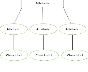
This is a type of data analysis that produces models that describe relevant data classes from a data set. The models are called classifiers and are used to predict a discrete value. Classification is a process of applying a target function to attributes in a data set which maps them to an already defined class label. The target function is known as the classification model. A classification model (Figure 2) is used for two reasons, namely descriptive modelling and predictive modelling. Descriptive modelling is used as an explanatory tool to differentiate between objects of different classes while predictive modelling is used to predict class labels of unknown records.
Figure 2. Classification model mapping attribute set to class label.
This method makes use of algorithms such as J48 decision tree, neural networks, Naïve Bayes, K-nearest neighbor, genetic algorithm, linear programming and statistics which serve as the classification model.
This approach is based on machine learning. The classification technique classifies items in a data set into a pre-defined set of groups. Data classification entails learning and classification. In learning the data set is analyzed by a classification algorithm and in classification, test data is used
to estimate the accuracy of classification rules. If the accuracy is accepted the rules are then applied to the new data set. [7]
3.2 J48 Decision Tree
Decision tree is one of the most widely used method for inductive inference on predictive data (supervised data). This method is used to classify categorical data based on their attributes. Decision tree as the name indicates is a tree like structure with a root node, branches and leaf nodes. Each node in a decision tree represents class label. A root node has no incoming edge with one or more or zero outgoing edges. Internal nodes have one incoming edge with one or more outgoing edges. Leaf nodes have one incoming edge but no outgoing edge. Root and internal nodes are the attributes of a data set and the leave nodes are the class labels (Figure 3).
Figure 3. Decision Tree
The decision tree technique is a fairly easy technique to understand and a popular one. It is widely used by researchers for its easiness and comprehensive nature in working with small and large data size and predicting values. The reasoning process can be converted to if-then rules. It is used to aid in decision making and as the name suggests, it is a tree –shaped structure. [8]
Decision tree learns a classification function which is used to determine the value of a dependent attribute given the values of the independent attributes. It is an advanced approach to knowledge discovery and data mining. Its benefits includes; easily understood by end user, handles a variety of data types like nominal, textual and numeric, processes missing and erroneous values, high performance with little effort and can be implemented on different platforms.
J48 decision tree is an updated version of ID3 algorithm. Its additional features include processing missing values, tree pruning, deriving rules and continuous values. In WEKA, it is an implementation C4.5 algorithm in java. The attribute to be predicted is the dependent variable since its value is determined by the values of other attributes which are the independent variables in the data set.
J48 uses a top-down, recursive divide and conquer method to generate the tree. An attribute is selected as the root node that is the attribute with the highest information gain. This is determined by the attribute that best segregates the instances in the training set. Instances are divided into subsets. This is repeated recursively at each branch until instances have the same class. [9]
[image:2.595.74.255.336.419.2]values are determined based on the classification of other instances. [10]
3.2
Neural network
A neural network is a brain analogy for processing information. This model is a biological inspiration of the behaviour of the brain. Neural networks have proven their ability in forecasting applications as a result of their “learning” ability. Artificial Neural Network (ANN)/ neural network which is a result of neural computing; a pattern recognition methodology for machine learning. Neural networks are popularly used for forecasting, pattern recognition, prediction and classification.
An ANN imitates the biological neural network but uses a limited set of concepts. Neural concepts are implemented as software simulations of parallel that involve processing of elements interconnected in a network structure. The artificial neuron receives input which represents the electrochemical impulses received by dendrites of the biological neurons from other neurons. The output of the artificial neuron resemble the signal sent out of the biological neuron through the axon. Artificial signals are changed to weight to emulate the physical change that occurs at a synapse.
The ANN receives the sum information from other neurons or as external input signal, performs a transformation and sends it to other neurons or as external output signals. Information is passed from neuron to neuron activating certain neurons based on information received. Hence the processing of information is a function of its structure.
[image:3.595.64.269.507.605.2]A neural network is made up of processing elements arranged in different ways to form a network structure. The basic processing unit is the neuron. Like many networks there are many ways in which these neurons can be arranged to form different topologies. The most common approach is the feedforward-backpropagation (backward propagation) paradigm. This approach allows neurons to link the output in one layer to the input in another but does not allow any feedback linkage.
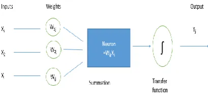
Figure 4. Processing of information in an ANN
The basic network structure of an ANN consists of the input, intermediate (hidden) and output layers. The intermediate layer is a layer of neurons that take inputs from previous layers, converts into output for more processing. The major concepts related to processing in an ANN are the inputs, outputs, weights, summation function and transfer function as shown in Figure 4 above. Below explains their roles.
Inputs are the attributes from a data set. For instance in a problem where it is to be decided if a student graduates or drops out, some of the attributes may be class attendance mid semester score, assignment scores. These attributes are presented in a numerical value as input.
Outputs are the results to the problem. The output could be graduate or dropout in the case of a student. This is also represented as a numeric value.
Weights or connection weights show the relative importance of each input to be processed which corresponds to the output. Also represented by a numerical value. They contain the learned patterns of recognition.
Summation function computes the weighted sums of all inputs. The function multiplies each input value by its weight and adds up the values for a weighted sum Y.
Transfer function adds up the inputs coming into a neuron from other neurons and produces an output based on the type of transfer function chosen. [11]
Multilayer Perceptron (MLP) is a feedforward Artificial Neural Network, mapping weighted input to output. It consist of several layers of nodes where all layers are fully connected. Each node is a neuron with a nonlinear activation function except for the input nodes. MLP trains network using supervised learning in backpropagation. Backpropagation algorithm is used in a feed forward layered network. Here neurons are in layers and sends signals forward while errors are propagated backwards. The error is the difference between the actual and the expected results.
3.3
K-Nearest Neighbor
The K- nearest neighbor (KNN) is one of the most common algorithms used in classification. It is a non-parametric lazy learning algorithm. It is non-parametric because it does not make assumptions on the given data. It is a lazy algorithm because it does not make use of training data points to do generalization. If there is any training data then it is minimal and used at the testing phase.
[image:3.595.320.532.522.637.2]When using KNN, data is in metric space. This can be scalar or multi-dimensional vectors. Distance is usually involved and Euclidean distance is mostly used though there are other methods of measuring distance. Each training data is a set of vectors with associated class labels. The vector is either positive or negative. A number “K” is given which indicates the number of neighbors to be considered. If K=1 then the algorithm is called nearest neighbor algorithm. (Figure 5)
Figure 5 K-Nearest Neighbors
When using KNN for classification, data points for training and a new unlabeled data for testing are given. The aim is to find a new class label for the new data point. The algorithm behaves differently depending on the value of K. [12]
The K- nearest neighbor algorithm is an instance based learner which compares new instances to instances seen in training set stored in memory instead of performing distinct generalization. The function is estimated locally and computed until instances are classified. Weights are assigned to neighbors such that close neighbors contribute more to the average than distant neighbors. Neighbors are taken from the training set where the class is known.
Training instances are vectors in multidimensional feature space with class labels. In the training phase the algorithm stores feature vectors and class labels. In the classification phase, K a constant defined by the user and a test instance is classified by giving the label which is most frequent among the k training instances closest to the test instance. Euclidean distance is the distance metric used for continuous variables.
4.
COMPARISON VARIABLES
In order to do a proper appraisal of the algorithms, that is MLP, J48 decision tree and k- nearest neighbor under the classification technique, they need to be compared based on particular variables to see which algorithm does the classification well. The main variables used in comparing algorithms are accuracy, speed, robustness, scalability and interpretability.
A comparison of classification analysis was done based on accuracy, speed and robustness; the ability of the algorithm to handle noise and missing values from the data set with various data sets on fourteen algorithms. It is mentioned that accuracy, comprehensibility, computational complexity, robustness, scalability, stability and interestingness is the criteria used in evaluating classifiers. [14]
Software used were WEKA, SPSS and Rosetta. The best accuracy obtained was 100% for C4.5, AIRS2P, IBK, CSCA, Logit Boost, Logistics, MLP, MLVQ, Naïve Bayes, SVM, and RSES. CSCA algorithm was always the slowest and the rest were of similar speed. Robustness comparisons were conducted on several data sets before and after missing values were cleaned. Results showed that the accuracy of the algorithms did not change dramatically with noise though CART was the most robust and RSES the least robust algorithm.
Accuracy can be divided into two that is classifier accuracy and predictor accuracy. Classifier accuracy is the ability to predict the class label while predictor accuracy is guessing the value of predicted attributes. It is the percentage of correctly classified attributes. It is calculated as the sum of correctly classified attributes divided by the total number of attributes from the sample.
Classifier accuracy is calculated by determining the percentage of instances placed correctly in a class. The confusion matrix details the accuracy of a solution to a classification problem. Given n classes, a confusion matrix is an m x n matrix where Cij indicates the number of instances
from D (data set) that were assigned to class Cij but where the
correct class is Ci. The best solution has zeros outside the
diagonal. [10]
In terms of speed, which is a measure of the time used in constructing the model and time spent in using the model, Naïve Bayes is the fastest followed by decision tree and then neural network. For interpretability, referring to the understanding and insight provided by the model at the end of a classification, the computation process in WEKA for decision tree and Naïve Bayes is understandable as compared
to the black box nature of neural network. Scalability is how efficiently the algorithm handles increasing data inputs.
5.
METHODOLOGY
The qualitative; descriptive and explanatory methods of research was used in this study to explain the process of data mining. The effect of a student’s academic history and category of SHS attended on his or her future performance is described. This includes the general performance of student from the various SHS categories. In addition to this, the relationship between student SHS aggregate and CWA was further explained.
Quantitatively, the WEKA tool kit was used in data pre-processing and classification. With respect to classification, three algorithms were used to mine the data obtained. MLP, J48 decision tree and KNN were used to predict and assess student performance. Results obtained from mining data with these algorithms were compared to evaluate the
performance of the algorithms based on accuracy, speed, robustness, scalability and interpretability. Hence the appraisal of the algorithms.
5.1
Sampling and Data Collection
The department of Computer Science of KNUST was chosen for this study. Undergraduate students pursuing a four year degree programme leading to an award of a Bachelor of Science in computer science who were admitted during the period of 2004 and 2015 were used.
The department had a population of 1425 students, out of which 525 students were used as a sample unit for the case study. The sample unit consisted of students admitted in 2009 to 2012 with CWA of 40 and above (Pass to First Class), regular admission status. The data consists of academic history and current academic records of students. Academic history consists of SHS aggregate of student, admitted aggregate used for admission. Current academic records is comprises of end of semester examination marks and final CWA.
5.2
Application of DM process
Step 1: Data Cleaning
The required data was collected in the form of two excel sheets in separate books. One sheet was the data of all admitted students from all colleges from 2004 to 2015. This sheet included irrelevant attributes such as old school code, exam number and program name. The second sheet was academic records of computer science students admitted within 2004 and 2015. This sheet had attributes such as course name, semester, course code and continuous assessment (which were all null). The data was cleaned by removing all erroneous and irrelevant attributes and instances from the data. This included removing duplicates.
Step 2: Data Integration
Data stored in the two separate excel books were brought together in one excel sheet. This gave one sheet with all the needed attributes and correct instances.
Step 3: Data selection and transformation
Only fields that were required for the data mining were selected. A few derived variables were selected and information for the variables were selected from the database.
STNO- student number is the unique number given to every student.
[image:5.595.64.268.196.520.2]Best6- SHS aggregate is the sum of the six best subjects a student does well in. The grading category is A1, B2, B3, C4, C5, C6, D7, E8 and F9. A1 being the best grade and F9 being the worst. To tell the overall performance of a student, six subjects a student performed well is selected and the numbers next to the letters are added up. The best aggregate for a student is 6 and the worst that still qualifies for admission into the university is 24.
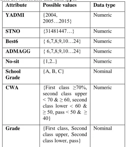
Table 1 Variable descriptions
Variable Description Possible values
YADMI Year of admission
{2004, 2005…2015}
STNO Student number {31481447…}
Best6 SHS Aggregate { 6,7,8,9,10…24}
ADMAGG Admitted aggregate
{ 6,7,8,9,10…24}
PName Program name {Regular,fee paying,less endowed}
School Previous SHS attended
{A, B, C}
Region Region of previous SHS attended
{Greater Accra, Brong Ahafo, Central, Volta, Eastern, Ashanti, Western, Northern, Upper East, Upper West}
CWA Cumulative
weighted average
{First class ≥70%, second class upper < 70 & ≥ 60, second class lower < 60 & ≥ 50, pass < 50 & ≥ 40}
ADMAGG- Admitted aggregate for admission is the SHS aggregate used to admit a student
PName- Program name tells how the student gained admission. Regular indicates the student met the required cut off point. Fee paying indicates the student did not meet the required cut off point but still qualifies for admission into the university (aggregate of 24 or better) and opts to pay extra fees if given admission. Last category is the less endowed, here the student does not necessarily meet the cutoff point but performs fairly well considering the category of SHS the student attended.
School- Previous SHS is the SHS the student attended. This is categorized as A, B and C. Category A school being the best of schools, followed by B and C.
Region- this indicates the region of the SHS.
CWA- Cumulative weighted average is the average performance of a student at the end of each semester. Grading is as follows: First class (70% and above), Second class upper division (69% to 60%), Second class Lower division (59% to 50%) and Pass (49 % to 40 %).
The region of the SHS was used to help classify the schools into A, B and C and the CWA of the students were converted into nominal values; First class, second class upper, second class lower and pass giving the attribute Grade. The excel sheet was convert to a Comma Separated Values (CSV) file which was then converted to an Attribute Relation File Format (ARFF) indicating the attributes and data type of the data set.
Below is a table showing the attributes and data types of the final data set.
Data mining algorithms were applied to extract patterns using WEKA tool kit. Classification data mining technique is used, applying J48 decision tree, artificial neural network (MLP) and K- nearest neighbor (IBK) algorithms to the data set prepared to predict student performance based on academic history. The relationship between SHS aggregate and CWA was determined resulting to patterns of student enrolment process. The same data set was applied to each algorithm hence comparing and contrasting the performance of each of the three algorithms.
Table 2.0 Attributes and data types
Attribute Possible values Data type
YADMI {2004,
2005…2015}
Numeric
STNO {31481447…} Numeric
Best6 { 6,7,8,9,10…24} Numeric
ADMAGG { 6,7,8,9,10…24} Numeric
No-sit {1,2..} Numeric
School Grade
{A, B, C} Nominal
CWA {First class ≥70%,
second class upper < 70 & ≥ 60, second class lower < 60 & ≥ 50, pass < 50 & ≥ 40}
Numeric
Grade {First class, Second class upper, Second class lower, pass}
Nominal
Step 4: Data Mining
Data mining algorithms were applied to extract patterns using WEKA tool kit. Classification data mining technique is used, applying J48 decision tree, artificial neural network (MLP) and K- nearest neighbor (IBK) algorithms to the data set prepared to predict student performance based on academic history. The relationship between SHS aggregate and CWA was determined resulting to patterns of student enrolment process. The same data set was applied to each algorithm hence comparing and contrasting the performance of each of the three algorithms.
Step 5: Pattern Evaluation
[image:5.595.321.534.305.552.2]Knowledge
Knowledge is the end product of data mining. At the end, knowledge of student performance, enrollment process and performance of the algorithms is produced.
5.3
Waikato Environment for Knowledge
Analysis (WEKA)
The University of Waikato in New Zealand developed the WEKA software written in Java which was used for this research. WEKA supports a wide range of algorithms and large data sets. It is an open source software issued by GNU General Public License. It contains tools for data- preprocessing, algorithms for classification, clustering, regression, visualization and association rules. Basically used for data analysis and predictive modelling. It has a graphical user interface making it easy to access the various functions.
The WEKA version 3.8.1 was used for its open source nature, portability since it was developed using Java hence runs on most computing platforms, its comprehensive tools and ease of use. To use WEKA, the collected data was converted to a csv or arff file format. [15]
6.
DATA ANALYSIS AND FINDINGS
The objective of the research was to find out
The algorithm better suited for predicting student performance
The correlation between SHS aggregate and the CWA of students
How well do students admitted from the various classes of SHS perform
Whether the admission requirements need to be revised
6.1
Algorithms for analyzing student
performance
A data set of 525 instances was used for analyzing student performance. The data set consisted of eight attributes, of which four were used to test the algorithms. The four attributes used are Best6, School grade, CWA and School Grade. The data set was split on a ratio of 60% for training and 40% for testing. The class label is Grade. The value to be predicted. J48 decision tree, IBK (KNN) and Multilayer perceptron (ANN) were run on the data.
6.1.1
J48 Model
Based on the training set of 315 instances (60%) the model built correctly classified 210 (40%) instances of the test data with an accuracy of 100%. This implies that all instances were correctly classified into their respective class values. The confusion matrix gives the details of the classification as follows;
88 instances correctly classified as second class lower
87 instances correctly classified as second class upper
24 instances correctly classified as pass
11 instances correctly classified as first Class
Figure 5. Classification Tree
6.1.2
KNN
K was set to 1 since the data set was not noisy and it gave the most accurate results.
Based on the training set of 315 (60%) instances, out of 210 (40%) test instances, 90.4726% was correctly classified and 9.5238% was incorrectly classified. The confusion matrix details the classification as follows;
82 instances correctly classified as second class lower and 4 incorrectly classified as second class upper
81 instances correctly classified as second class upper and 4 instances incorrectly classified as second class lower
22 instances correctly classified as pass and 2 instances incorrectly classified as second class lower
5 instances correctly classified as First class and 6 instances incorrectly classified as second class upper.6.1.3
MLP
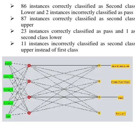
MLP correctly classified 93.3333% of test set and incorrectly classified 6.6667%. The confusion matrix gives the details as follows;
86 instances correctly classified as Second class Lower and 2 instances incorrectly classified as pass
87 instances correctly classified as second class upper
23 instances correctly classified as pass and 1 as second class lower
[image:6.595.317.540.469.676.2] 11 instances incorrectly classified as second class upper instead of first class
Figure 6. Classification using MLP
6.3 Performance of various classified
schools
The student data sample was further divided according to the class of schools, A, B and C. This was to study and compare the performance of the classified schools based on the best 6 and CWA.
For Class A Schools the correlation between best6 and CWA is 0.1745. There is a direct relation between best 6 and CWA but it is weak.
Class B Schools had a correlation of 0.3779 between best6 and CWA. There is a direct relation between best 6 and CWA but it is weak.
Class C Schools the correlation between best6 and CWA is 0.4589. There is a direct relation between best 6 and CWA but it is weak.
6.4 Prediction of student performance
For J48 predictions, students performed according to the predicted values with 1 being the greatest difference and 0 the least. All instances were correctly classified, thus 100%.For KNN predictions, students performed according to the predicted values with 0.994 being the greatest difference and 0.002 the least. There was a 96.3768% of correctly classified instances and 3.6232% of incorrectly classifies instances.
For MLP Predictions, students performed according to the predicted values with 0.997 being the greatest difference and 0 the least. There were 84.7826% of correctly classified instances and 15.2174% of incorrectly classifies instances.
6.5 Comparisons of Algorithms
The performance of J48 decision tree, KNN (IBK) and MLP were compared based on accuracy, speed, robustness, scalability and interpretability of the algorithms. Three student data samples were used. Each data had a different number of instances.
Accuracy and scalability
J48 performs significantly better than IBK and MLP on all data sets. The classifier accuracy increases with lager data set. While for IBK and MLP, the classifier accuracy decreased for student sample 2 and increased for student sample 3. J48 had a predictor accuracy of 100%, IBK had a predictor accuracy of 96.3768% and MLP had a predictor accuracy of 84.7826%.
Speed and robustness
J48 and IBK took zero seconds to build model and test the model on test split while MLP took 0.94 seconds to build model and zero seconds to test model on test split.
A student dataset with noise and missing values was used. J48 had an accuracy of 98.9011% with a speed of 0.07 sec to build model and 0.01 sec to test model on test split. IBk had an accuracy of 80.2198% with a speed of 0 sec to build model and 0.006 to test model on test split. MLP had an accuracy of 92.3077% with a speed of 1.32sec to build model and 0 sec to test model on test split.
Interpretability
J48 had the best interpretability by being able to classify most instances correctly into First class. Second class upper, second class lower and pass with 100 % classifier and predictable accuracy. IBk had 90.5238% classifier accuracy and 96.3768% predictor accuracy. While MLP had 93.3333% classifier accuracy with a predictor accuracy of 84.7826%.
7.
CONCLUSION
There is no single answer as to the best algorithm that should be used to mine student data. The algorithm that would be used highly depends on the task to be performed. J48 algorithm produced the best classifier and predictor models with 100% accuracy but it could not predict the exact values. It had the greatest difference between predicted and actual values. IBK had the least difference between its predicted values and the actual. While MLP had a relatively poorer predictor accuracy but with better difference between actual and predicted values.
J48 decision tree performs better with increasing data size as the classifier accuracy increases followed by IBK and then MLP. J48 and IBK are faster at building and testing the model as compared to MLP. In terms of robustness, all algorithms handled the noise better since the percentage of accuracy did not reduce drastically.
J48 had the best interpretability as it correctly classified all instances. Amongst the three algorithms J48 decision tree is the best even though the other algorithms are good enough for analyzing and predicting student performance.
Students admitted with the best SHS aggregate do not often graduate with a first class. After been admitted, all students have an equal chance of obtaining a first class. When performance is analysed according to various classes of schools, it was noted that student from Class C schools generally perform better than students from class B and A schools by showing high correlation with respect to best6 and graduating class (section 6.3).
It is not straight forward that students that attain best SHS aggregate would graduate with a first class or at least a second class upper. More specifically for the Department of Computer Science, very few first class students have been produced over the period under study.
Current admission requirements may have actually denied students with much potential to gain admission on the basis of their SHS aggregate which in itself is not full measure of a student’s potential. Wider scope of data that covers other parameters such as parents’ level of education, economic background, environment at home, occupation, physical disability and health related issues could be covered in future study for better or more accurate analytics.
8.
RECOMMENDATION
We strongly recommend that other researchers adopt J48, MLP and IBK algorithms to mine students’ performance using WEKA tool to explore more predictor variables that contribute to the choice of parents/guardians, students and higher educational institutions to improve quality of education and national development.
Most of the admitted students come from the class A and B schools with the best of the SHS aggregate but do not all of them live up to expectation (See Section 6.3). Hence it is recommended that more admission slots should be allocated to students coming from Class C schools.
average when admitted to university education. Parents and guardians whose dream is only to get their ward into Class A schools should rethink and consider some selected Class B and Class C schools if they want their ward to be amongst outstanding graduands to fulfil their career dreams.
Based on this research, it is clear that academic performance history is only one factor of a student amongst many that determine the success of a student in the university. Other factors that help determine the performance of students are parents’ level of education, economic background, environment at home, occupation, physical disability and health related issues. These are usually captured in the admission form but not entered into the database. It is therefore recommended that the admission team input such details into the database for a more holistic research to be conducted in future works.
9.
REFERENCES
[1]. Baradwaj, B.K. and Pal, S. (2012). Mining educational data to analyze students' performance. International Journal of Advanced Computer Science and Applications. (IJACSA), Vol 2 No. 6 pp 63-69
[2]. Jing, L. (2004). Data Mining Applications in Higher Education. Executive report, SPSS Inc, pp.22-24. [3]. Ahmed, A. B. E. D. and Elaraby, I. S. (2014). Data
Mining: A prediction for Student's Performance Using Classification Method. World Journal of Computer Application and Technology, 2(2), 43-47.
[4]. Campagni, R., Merlini, D., Sprugnoli, R. and Verri, M. C. (2015). Data mining models for student careers. Expert Systems with Applications, 42(13), 5508-5521. [5]. Romero, C. and Ventura, S. (2010). Educational data
mining: a review of the state of the art. IEEE Transactions on Systems, Man, and Cybernetics, Part C (Applications and Reviews), 40(6), pp.601-618
[6]. Pal, A.K. and Pal, S. (2013). Analysis and mining of educational data for predicting the performance of
students. International Journal of Electronics Communication and Computer Engineering, 4(5), pp.1560-1565.
[7]. Bhardwaj, B.K. and Pal, S. (2012). Data Mining: A prediction for performance improvement using classification. arXiv preprint arXiv:1201.3418. International Journal of Computer Science and Information Security (IJSCIS), Vol 9 No. 4
[8]. Shahiri, A. M. and Husain, W. (2015). A review on predicting student's performance using data mining techniques. Procedia Computer Science, 72, 414-422. [9]. Bhargava, N., Sharma, G., Bhargava, R. and Mathuria,
M. (2013). Decision tree analysis on j48 algorithm for data mining. Proceedings of International Journal of Advanced Research in Computer Science and Software Engineering, 3(6).
[10].Patil, T.R. and Sherekar, S.S. (2013). Performance analysis of Naive Bayes and J48 classification algorithm for data classification. International Journal of Computer Science and Applications, 6(2), pp.256-261.
[11].Thirumuruganathan, S. (2010). A detailed introduction to K-nearest neighbor (KNN) algorithm. Algorithm. https://saravananthirumuruganathan. wordpress. com/2010/ 05/17/a-detailed-introduction-to-k-nearest-neighbor-knn-algorithm/ Accessed on 30th April 2016 [12].Phyu, T.N. (2009). March. Survey of classification
techniques in data mining. In Proceedings of the International MultiConference of Engineers and Computer Scientists (Vol. 1, pp. 18-20).
[13].Dogan, N. and Tanrikulu, Z. (2013). A comparative analysis of classification algorithms in data mining for accuracy, speed and robustness. Information Technology and Management, 14(2), pp.105-1