Optimization of Markov Random Fields in Computer Vision

Fields in Computer Vision

Thalaiyasingam Ajanthan

A thesis submitted for the degree of

Doctor of Philosophy

The Australian National University

November 2017

c

I hereby declare that this submission is my own work (based on publications in collaboration with the co-authors where due acknowledgement is made) and that, to the best of my knowledge, it contains no material previously published or written by another person nor material which to a substantial extent has been accepted for the award of any other degree or diploma at ANU or any other educational institution, except where due acknowledgment has been made.

I also declare that all sources used in this thesis have been fully and properly cited.

First and foremost, I would like to express my sincere gratitude to my primary super-visor, Prof. Richard Hartley, for his guidance, motivation, and support throughout my PhD research. It has been an absolute privilege to work with Richard, and this work would not have been possible without his contagious enthusiasm for research. Thank you, professor, for being immensely helpful in many ways both in academic and personal matters. In particular, thank you for inspiring me to work on the ex-citing field of MRF optimization. Your upcoming book onSolution of Markov Random Fieldshas been instrumental in reducing my learning time.

I am equally grateful to my co-supervisors, As.Prof. Hongdong Li (panel chair) and Dr. Mathieu Salzmann. Thank you for giving me valuable pointers and ideas, shaping my research and carefully reviewing all manuscripts I produced during my PhD. I am indebted to Mathieu for his continuous guidance even after he moved to EPFL, Switzerland. I would also like to thank the other researchers at Data61 and ANU for their feedback on my research during various seminars and reading groups. I would like to thank Prof. Philip Torr for offering me to visit his group at the University of Oxford for almost 5 months and introducing me to exciting new prob-lems. I am deeply grateful to As.Prof. Pawan Kumar for being a great mentor and working with me during my time in Oxford. I would also like to thank my collabo-rators, Alban and Rudy and other colleagues at the University of Oxford for warmly welcoming me to their circle.

I am grateful to my colleagues at Data61 and ANU, past and present, who created a wonderful research environment. Especially, I would like to convey my gratitude to Sadeep (for introducing me to Mathieu and guidance on various matters), Ka-malaruban (for the countless things he has done for me), Zeeshan, Arash, Saeed, Masoud and Samitha.

I graciously acknowledge and appreciate the financial support from the Aus-tralian National University, NICTA (now Data61, CSIRO) and the AusAus-tralian Gov-ernment for my PhD research. Their scholarships and generous travel grants have allowed me to focus on my research without having to worry about financial support. I am indebted to my teachers at the University of Moratuwa, especially, Dr. Ranga Rodrigo for constantly encouraging me to pursue a PhD in computer vision. I am equally indebted to my teachers back in my hometown Jaffna, Sri Lanka.

Most importantly, I would like to express my gratitude to my family and friends. Thank you, my father late Thalaiyasingam, mother Jeyaluxmy, and brother Sugan-than, for your unconditional love and support. This thesis is dedicated to you. Fi-nally, my dear friends (in Canberra and other parts of the world), thank you for making my life fun-filled.

A large variety of computer vision tasks can be formulated using Markov Random Fields (MRF). Except in certain special cases, optimizing an MRF is intractable, due to a large number of variables and complex dependencies between them. In this thesis, we present new algorithms to perform inference in MRFs, that are either more efficient (in terms of running time and/or memory usage) or more effective (in terms of solution quality), than the state-of-the-art methods.

First, we introduce a memory efficient max-flow algorithm formulti-label submod-ularMRFs. In fact, such MRFs have been shown to be optimally solvable using max-flow based on an encoding of the labels proposed by Ishikawa, in which each variable Xi is represented by `nodes (where`is the number of labels) arranged in a column. However, this method in general requires 2`2 edges for each pair of neighbouring variables. This makes it inapplicable to realistic problems with many variables and labels, due to excessive memory requirement. By contrast, our max-flow algorithm stores 2` values per variable pair, requiring much less storage. Consequently, our algorithm makes it possible to optimally solve multi-label submodular problems in-volving large numbers of variables and labels on a standard computer.

Next, we present a move-making style algorithm for multi-label MRFs with ro-bust non-convex priors. In particular, our algorithm iteratively approximates the original MRF energy with an appropriately weighted surrogate energy that is easier to minimize. Furthermore, it guarantees that the original energy decreases at each it-eration. To this end, we consider the scenario where the weighted surrogate energy is multi-label submodular (i.e., it can be optimally minimized by max-flow), and show that our algorithm then lets us handle of a large variety of non-convex priors.

Finally, we consider the fully connected Conditional Random Field (dense CRF) with Gaussian pairwise potentials that has proven popular and effective for multi-class semantic segmentation. While the energy of a dense CRF can be minimized ac-curately using a Linear Programming (LP) relaxation, the state-of-the-art algorithm is too slow to be useful in practice. To alleviate this deficiency, we introduce an effi-cient LP minimization algorithm for dense CRFs. To this end, we develop a proximal minimization framework, where the dual of each proximal problem is optimized via block-coordinate descent. We show that each block of variables can be optimized in a timelinearin the number of pixels and labels. Consequently, our algorithm enables efficient and effective optimization of dense CRFs with Gaussian pairwise potentials. We evaluated all our algorithms on standard energy minimization datasets con-sisting of computer vision problems, such as stereo, inpainting and semantic seg-mentation. The experiments at the end of each chapter provide compelling evidence that all our approaches are either more efficient or more effective than all existing baselines.

Acknowledgements vii

Abstract ix

1 Introduction 1

1.1 Some Computer Vision Applications . . . 2

1.1.1 The Labelling Problem . . . 2

1.1.2 Stereo Correspondence Estimation . . . 2

1.1.3 Image Denoising and Inpainting . . . 2

1.1.4 Semantic Segmentation . . . 3

1.2 Limitations of Existing Algorithms . . . 4

1.3 Contributions . . . 6

1.4 Thesis Outline . . . 6

1.5 Publications . . . 7

1.5.1 Under Review . . . 8

1.5.2 Conferences . . . 8

2 Background and Preliminaries 9 2.1 Markov Random Fields . . . 9

2.1.1 Conditional Random Fields . . . 12

2.1.2 Optimizing an MRF . . . 13

2.1.3 MRF Optimization Algorithms . . . 13

2.2 Binary MRF Optimization . . . 14

2.2.1 Pseudo-Boolean Functions . . . 15

2.2.2 Submodular Functions . . . 15

2.2.3 Graph Representability . . . 16

2.2.3.1 Representing the Binary MRF Energy in anst-graph . . 18

2.2.4 Min-Cut and Max-Flow . . . 19

2.2.5 Non-Submodular MRFs . . . 20

2.3 Multi-Label MRF Optimization . . . 20

2.3.1 Multi-Label Graph . . . 21

2.3.2 Ishikawa Algorithm . . . 21

2.3.3 Move-Making Algorithms . . . 26

2.3.3.1 α-expansion . . . 27

2.3.3.2 Convexα-expansion . . . 30

2.3.3.3 Other Move-Making Algorithms . . . 31

2.3.4 Linear Programming Relaxation . . . 32

2.3.4.1 Marginal Polytope . . . 33

2.3.4.2 Local Polytope . . . 35

2.3.4.3 Message Passing and Reparametrization . . . 38

2.3.4.4 Optimality of Message Passing on Tree Structured MRFs 40 2.3.4.5 Tree Reweighted Message Passing . . . 42

2.3.5 Other Continuous Relaxations . . . 44

2.4 Summary . . . 45

3 Memory Efficient Max-Flow for Multi-Label Submodular MRFs 47 3.1 Introduction . . . 47

3.2 Preliminaries . . . 48

3.2.1 The Ishikawa Graph . . . 48

3.2.2 Max-Flow . . . 50

3.2.3 Our Idea . . . 50

3.3 Memory Efficient Flow Encoding . . . 51

3.3.1 Flow Reconstruction . . . 53

3.4 Polynomial Time Memory Efficient Max-Flow . . . 54

3.4.1 Finding an Augmenting Path . . . 54

3.4.2 Augmentation . . . 55

3.4.3 Summary . . . 56

3.4.4 Time Complexity Analysis . . . 57

3.5 Efficient Algorithm . . . 60

3.5.1 Efficiently Finding an Augmenting Path . . . 61

3.5.2 Augmentation in the Block-Graph . . . 63

3.5.3 Summary . . . 66

3.6 Equivalence with Message Passing . . . 67

3.6.1 The Optimal Message Passing Problem . . . 68

3.6.2 Max-Flow Solves the Optimal Message Passing Problem . . . 68

3.6.3 Flow-Loop as a Reparametrization . . . 70

3.7 Related Work . . . 72

3.7.1 Max-Flow-based Methods . . . 72

3.7.2 LP Relaxation-based Methods . . . 72

3.8 Experiments . . . 73

3.8.1 MEMF Analysis . . . 74

3.8.2 Robust Regularizer . . . 75

3.8.3 Parallelization . . . 76

3.9 Discussion . . . 78

4 Iteratively Reweighted Graph-Cut for Multi-Label MRFs with Non-Convex Priors 81 4.1 Introduction . . . 81

4.2 Iteratively Reweighted Minimization . . . 82

4.2.1 Relationship to the Majorize-Minimize Framework . . . 85

4.4 Iteratively Reweighted Graph-Cut . . . 87

4.4.1 MRF with Pairwise Interactions . . . 87

4.4.2 Choice of Functionsgandhb . . . 90

4.4.3 Hybrid Strategy . . . 92

4.5 Related Work . . . 92

4.5.1 Approximate MRF Optimization Algorithms . . . 92

4.5.2 IRLS-based Methods . . . 93

4.6 Experiments . . . 93

4.6.1 Stereo Correspondence . . . 94

4.6.2 Image Inpainting . . . 96

4.6.2.1 Tackling Large Scale Problems . . . 96

4.6.3 Summary . . . 97

4.6.4 IRGC Analysis . . . 98

4.7 Discussion . . . 100

5 Efficient Linear Programming for Dense CRFs 105 5.1 Introduction . . . 105

5.2 Preliminaries . . . 106

5.2.1 Dense CRF Energy Function . . . 107

5.2.2 Gaussian Pairwise Potentials . . . 107

5.2.3 Integer Programming Formulation . . . 108

5.2.4 Linear Programming Relaxation . . . 108

5.2.5 Proximal Minimization Algorithm . . . 109

5.2.6 The Frank-Wolfe Algorithm . . . 110

5.3 Proximal Minimization for LP Relaxation . . . 112

5.3.1 Dual Formulation . . . 113

5.3.2 Algorithm . . . 116

5.3.2.1 Optimizing overβandγ . . . 117

5.3.2.2 Optimizing overα . . . 119

5.3.2.3 Summary . . . 122

5.4 Fast Conditional Gradient Computation . . . 122

5.4.1 Original Filtering Method . . . 123

5.4.2 Modified Filtering Method . . . 124

5.4.2.1 Adaptive Version . . . 126

5.5 Related Work . . . 127

5.5.1 Dense CRF . . . 127

5.5.2 LP Relaxation . . . 128

5.5.3 Frank-Wolfe . . . 128

5.6 Experiments . . . 129

5.6.1 Accelerated Variants . . . 129

5.6.2 Implementation Details . . . 129

5.6.3 Segmentation Results . . . 130

5.6.3.1 Results with the Parameters Tuned for DCneg . . . 131

5.6.3.3 Summary . . . 135

5.6.4 PROX-LP Analysis . . . 136

5.6.4.1 Statistics of More Images . . . 136

5.6.4.2 Effect of the Proximal Regularization Constant . . . 137

5.6.5 Modified Filtering Method . . . 137

5.7 Discussion . . . 138

6 Conclusion 141 6.1 Contributions . . . 141

6.2 Future Directions . . . 143

Bibliography 145

1.1 An example of stereo correspondence estimation. . . 3

1.2 An example of image denoising and inpainting. . . 3

1.3 Examples of semantic segmentation. . . 4

2.1 Example of an MRF represented by an undirected graph. . . 10

2.2 Sparse neighbourhood structures often used in computer vision. . . 11

2.3 An example of image inpainting with and without pairwise potentials. 12 2.4 Example of anst-graph. . . 17

2.5 The st-graph representation of a binary MRF energy function. . . 19

2.6 Example of a multi-label graph. . . 21

2.7 The multi-label submodular condition illustrated using the multi-label graph. . . 22

2.8 Examples of convex priors. . . 23

2.9 Example of an Ishikawa graph. . . 24

2.10 Example of anα-expansion iteration. . . 28

2.11 Thest-graph construction for theα-expansion algorithm. . . 29

2.12 Examples of metric and semi-metric potentials. . . 30

2.13 An example binary labelling problem of convexα-expansion. . . 31

2.14 A labelling is represented in the multi-label graph for a linear MRF. . . 33

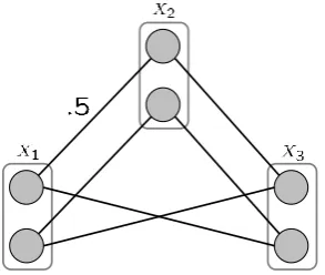
2.15 The marginal polytopeΩof an example binary MRF with 3 nodes. . . . 34

2.16 The local polytope is a convex outer bound of the marginal polytope. . 36

2.17 An MRF example where a fractional labelling is a vertex of the local polytope. . . 37

2.18 An elementary reparametrization. . . 39

2.19 Message passing on a linear MRF with 3 nodes. . . 41

2.20 A valid tree decomposition, where each subtree is chosen to be a span-ning tree. . . 43

3.1 Example of an Ishikawa graph. . . 49

3.2 An example of two equivalent flow representations with the same exit-flows. . . 52

3.3 Given initial Ishikawa capacities and the set of exit-flows, flow recon-struction is formulated as a max-flow problem. . . 53

3.4 Block-graph construction. . . 61

3.5 A loop in the block-graph is equivalent to the summation of flow-loops in the Ishikawa graph. . . 64

3.6 An augmentation operation is broken down into a sequence of

flow-loops and a subtraction along the last column. . . 64

3.7 Augmenting path in the block-graph and its corresponding directed acyclic graph in the Ishikawa graph. . . 66

3.8 A flow-loop in the Ishikawa graph and its equivalent reparametriza-tion in the multi-label graph. . . 71

3.9 Left and right images of the stereo instance from the KITTI dataset. . . 73

3.10 Lengths of augmenting paths found by our algorithm for the Tsukuba stereo instance. . . 75

3.11 Running time plots (in logarithmic scale) by changing the image size and by changing the number of labels, for Tsukuba and Penguin. . . 76

3.12 Percentage of time taken by each subroutine. . . 77

3.13 Our algorithm can be accelerated using the parallel max-flow technique. 77 4.1 Illustration of Lemma 4.2.1. . . 84

4.2 Example of an Ishikawa graph for convex priors. . . 90

4.3 Plots ofθ, gandhbwithθ(z) =hb◦g(z). . . 91

4.4 Disparity maps obtained with IRGC+expansion. . . 96

4.5 Energy vs time plots for the algorithms for some stereo problems and an inpainting problem. . . 98

4.6 Inpainted images for Penguin. . . 99

5.1 An iteration of the Frank-Wolfe algorithm illustrated using a 3D example.110 5.2 A 2-dimensional hyperplane tessellated by the permutohedral lattice. . 124

5.3 Original and modified filtering methods. . . 126

5.4 Assignment energy as a function of time with the parameters tuned for DCneg for an image in MSRC and Pascal. . . 132

5.5 Segmentation results with the parameters tuned for DCneg for some images in MSRC and Pascal. . . 133

5.6 Assignment energy as a function of time with the parameters tuned for MF for an image in MSRC and Pascal. . . 134

5.7 Segmentation results with the parameters tuned for MF for some im-ages in MSRC and Pascal. . . 135

5.8 Assignment energy as a function of time with the parameters tuned for DCneg for some images in MSRC. . . 137

5.9 Assignment energy as a function of time for an image in MSRC, for different values of η. . . 138

3.1 Memory consumption and running time comparison with state-of-the-art baselines for quadratic regularizer. . . 74 3.2 Memory consumption and running time comparison with

state-of-the-art baselines for Huber regularizer. . . 78 4.1 Functions g and hb corresponding to a given θ(z), such that θ(z) is

convex ifz≤κand concave otherwise. . . 91 4.2 Pairwise potential used for the stereo problems. . . 94 4.3 Comparison of the minimum energies and execution times for stereo

problems with metric prior. . . 95 4.4 Comparison of the minimum energies and execution times for stereo

problems with semi-metric priors. . . 95 4.5 Comparison of the minimum energies and execution times on Tsukuba

with a corrupted Gaussian prior. . . 97 4.6 Comparison of minimum energies and execution times for the

trun-cated quadratic prior on two inpainting problems. . . 97 4.7 Memory consumption and running time comparison of IRGC+expansion

with either the BK method or our MEMF algorithm as subroutine. . . . 100 4.8 Quality of the minimum energies. . . 100 4.9 Comparison of the minimum energies and execution times for Tsukuba

with different values ofκ. . . 101 4.10 Comparison of the minimum energies and execution times for Penguin

with different values ofκ. . . 102 5.1 Parameters tuned for MF and DCneg on the MSRC and Pascal

valida-tion sets using Spearmint. . . 130 5.2 Results on the MSRC and Pascal datasets with the parameters tuned

for DCneg. . . 132 5.3 Results on the MSRC and Pascal datasets with the parameters tuned

for MF. . . 134 5.4 Best segmentation results of each algorithm with their respective

pa-rameters, the average time on the test set and the segmentation accuracy.136

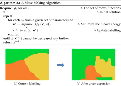
2.1 A Move-Making Algorithm . . . 28

3.1 Memory Efficient Max-Flow (MEMF) - Polynomial Time Version . . . . 56

3.2 Memory Efficient Max-Flow (MEMF) - Efficient Version . . . 67

4.1 Iteratively Reweighted Minimization . . . 85

4.2 Iteratively Reweighted Graph-Cut (IRGC) . . . 89

5.1 The Frank-Wolfe Algorithm . . . 112

5.2 Proximal Minimization of LP (PROX-LP) . . . 116

5.3 Original Filtering Method . . . 125

5.4 Modified Filtering Method . . . 127

Introduction

Computer vision aims at building artificial systems that extract useful information (e.g., objects, their boundaries, motion and 3D information, etc.) from images and videos. Unlike humans, this is an extremely difficult task for a computer, because it needs to interpret image data (a bunch of matrices) to descriptions of the world. Due to the inherent uncertainty, many of these problems are formulated as inference in probabilistic graphical models.

Probabilistic Graphical Models (PGM) [Koller and Friedman, 2009] describe mul-tivariate probability distributions which factor according to a graph structure. Specif-ically, the underlying graph expresses the conditional dependence structure between random variables that hold in the encoded distribution. Two branches of graphical models are commonly used, namely, Bayesian networks and Markov Random Fields (MRF). These two models differ in the graph structure (i.e., in the set of indepen-dences they can encode), namely, for Bayesian networks, the underlying graph is directed and acyclic and in the case of MRFs, it is an undirected graph.

In this thesis, we focus on Markov random fields. Inference in an MRF is often expressed as a discrete optimization problem, where the dependencies of the vari-ables are encoded in a graph. Such problems are often referred to as combinatorial optimization1problems. This combinatorial nature makes it a theoretically interesting research problem and in general, the optimization is NP-hard, i.e., computationally intractable [Nemhauser and Wolsey, 1988]. Furthermore, many computer vision ap-plications of MRF have millions of variables and complex dependencies between them, making the inference more challenging. Therefore, to develop practically ef-ficient algorithms, researchers either restrict themselves to a certain class of MRFs (e.g., restricted graph structures and restricted cost functions) or focus on developing approximate algorithms.

The existing MRF optimization algorithms in computer vision can be catego-rized into three groups: 1) exact combinatorial algorithms for certain special cases; 2) move-making style algorithms which iteratively minimize surrogate problems; 3) continuous relaxation based methods which make use of convex optimization tech-niques. In this thesis, we make contributions in all three categories by introducing

1_{Combinatorial optimization is the study of optimization on discrete and combinatorial objects (e.g.,}

graphs).

new algorithms that are either more efficient (in terms of running time and/or mem-ory usage) or more effective (in terms of solution quality), than the state-of-the-art methods.

Before presenting our contributions, we briefly review a few examples of com-puter vision problems and show how they can be formulated as discrete labelling problems.

1

.

1

Some Computer Vision Applications

Here we briefly discuss some core computer vision applications that are usually for-mulated as MRFs and hence a discrete labelling problem. We will formally define an MRF and related inference algorithms in Chapter 2. However, for better understand-ing, we first define the labelling problem and then turn to the examples.

1.1.1 The Labelling Problem

The objective of the labelling problem is to classify a set of nodes V = {1, 2, . . . ,n} by assigning a label to each node from a label set L. In this thesis, we consider the label set L to be discrete and finite. In particular, the labelling can be represented by a functionx : V → L, and the label assignment of a nodeiis usually denoted as xi =x(i).

Note that there are|L|n_{possible label configurations. In a typical computer vision} problem, each label configuration has a cost associated with it (called an energy), and the objective is to find the label configuration with the minimum cost (called energy minimization). Except in certain special cases, one has to check all|L|n_possible configurations, making it an intractable problem. It will be seen in the next chapter that a Markov random field can be expressed as a discrete labelling problem.

1.1.2 Stereo Correspondence Estimation

In stereo correspondence estimation [Scharstein and Szeliski, 2002], a pair of cali-brated images are given, a left image and a right image, and the objective is to find thedisparity between those two images. Here, by calibrated, we mean that the two images are aligned up to a horizontal displacement only, and disparity means that the horizontal displacement of a pixel in the left image to the corresponding pixel in the right image. Hence, it is a labelling problem whereV is the set of pixels and L is the set of possible disparities. See Figure 1.1 for an example. In fact, given the disparity, the depth can be determined [Hartley and Zisserman, 2003] and therefore stereo estimation is essential to obtain 3D information of a scene.

1.1.3 Image Denoising and Inpainting

(a) Left image (b) Right image (c) Disparity map

Figure 1.1: An example of stereo correspondence estimation. Given the left and right images, we need to find the disparity map between them.

(a) Corrupted image (b) Restored image

Figure 1.2: An example of image denoising and inpainting. Given the noisy image with corrupted pixels, we need to restore the original image.

acquisition), the objective is to restore the original content of the image. In this case, one needs to estimate the pixel intensities. Therefore, this is a labelling problem where V is the set of pixels and Lis the set of intensities ({0, . . . , 255}in case of a gray scale image). See Figure 1.2 for an example.

1.1.4 Semantic Segmentation

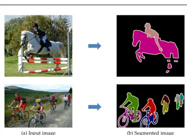
(a) Input image (b) Segmented image

Figure 1.3: An example of object segmentation (top) and instance segmentation (bottom). Given the input image, we need to segment the objects (or instances) and label them. The color indicates the class (or instance) label.

1

.

2

Limitations of Existing Algorithms

Note that, in most vision applications, there is a variable in the MRF corresponding to each pixel in the image2. Therefore, a typical MRF has millions of variables and complex dependencies between them, defined by the underlying graph structure. Usually, in computer vision, a sparse connectivity is assumed (e.g., 4-connected or 8-connected neighbourhood structure). However, as will be seen later, in certain applications, dense connectivity (i.e., each node is connected to every other node) is preferred [Krähenbühl Philipp, 2011]. In fact, the difficulty of optimizing an MRF depends on the underlying graph structure and the form of the cost function used to model the problem.

Over the past decade, various MRF optimization algorithms have been intro-duced. They can be categorized into three groups: 1) exact algorithms for certain special cases; 2) move-making style algorithms; 3) continuous relaxation based meth-ods. In fact, exact optimization is possible only for certain restricted cases (e.g., submodular energy functions and tree structured MRFs). For example, when the MRF energy is submodular (defined later in Chapter 2), it can be optimized using the max-flow algorithm [Kolmogorov and Zabin, 2004]. However, for general MRFs,

2_{Superpixels (polygonal parts in the image resulting from partitioning) based MRFs have also been}

one has to settle for an approximate algorithm. One class of algorithms approximate the original MRF energy by iteratively minimizing a surrogate energy (usually a sub-modular energy), and guarantee a monotonic decrease in the original MRF energy. At each iteration, such an algorithm moves from the current labelling to a lower energy labelling, and therefore this class of algorithms are referred to as move-making algo-rithms [Boykov et al., 2001]. On the other hand, the discrete labelling problem can be relaxed to a continuous optimization problem (such as a linear program [Chekuri et al., 2004; Werner, 2007] or a quadratic program [Ravikumar and Lafferty, 2006]) and tackled using convex optimization techniques.

We now point out some limitations of the existing algorithms in each of the above mentioned category, and, in the next section, we briefly discuss how our algorithms overcome these limitations.

1. Ishikawa [Ishikawa, 2003] introduced a max-flow-based method to globally minimize the energy ofmulti-label submodularMRFs (defined later). In the gen-eral case, however, this method requires 2`2 <sub>directed edges (where ` is the</sub> number of labels) for each pair of neighbouring variables. For instance, for a 1000×1000, 4-connected image with 256 labels, it would require approximately 1000×1000×2×2562×2×4 ≈ 1000 GB of memory to store the edges (as-suming 4 bytes per edge). Clearly, this is beyond the storage capacity of most computers. Even though the optimal solution can be obtained in polynomial time, due to excessive memory requirement, this algorithm cannot be applied to realistic problems with many variables and labels.

2. As we pointed out previously, in most scenarios one has to rely on an approx-imate algorithm to optimize a multi-label MRF. Even though move-making al-gorithms [Boykov et al., 2001] have proven successful for specific problems (e.g., metricpriors), there does not seem to be a single algorithm that performs well with different non-convex priors. In particular, while widely acknowledged as highly effective in computer vision, optimizing multi-label MRFs with robust non-convex priors, such as the truncated quadratic, the Cauchy function and the corrupted Gaussian still remains challenging.

3. The fully connected Conditional Random Field3 (dense CRF) with Gaussian pairwise potentials has proven popular and effective for multi-class semantic segmentation [Krähenbühl Philipp, 2011]. For such problems, the Linear Pro-gramming (LP) relaxation provides strong theoretical guarantees on the quality of the solution [Kleinberg and Tardos, 2002; Kumar et al., 2009]. Even though there are efficient algorithms for LP relaxation of sparse CRFs [Kolmogorov, 2006], optimizing a dense CRF is extremely challenging and the state-of-the-art algorithm [Desmaison et al., 2016a] is too slow to be useful in practice.

3_{From the optimization point of view, the CRF and the MRF are identical. This will become clear}

1

.

3

Contributions

In this thesis, we introduce new algorithms for MRF optimization, targeting com-puter vision applications. Our algorithms are either more efficient (in terms of run-ning time and/or memory usage) or more effective (in terms of solution quality), than the state-of-the-art methods. Furthermore, we briefly discuss how our algo-rithms address the limitations of the existing ones.

1. We introduce a memory efficient variant of the max-flow algorithm for multi-label submodular MRFs. Specifically, our max-flow algorithm stores only two

`-dimensional vectors (where`is the number of labels) per variable pair instead of the 2`2 <sub>edge capacities of the standard max-flow algorithm. Consequently,</sub> we reduce the memory requirement of the max-flow algorithm by O(`) for Ishikawa type graphs, while not compromising on optimality. As a result, our approach lets us optimally solve much larger problems on a standard computer. 2. We present a move-making style algorithm for multi-label MRFs with robust non-convex priors. In particular, our algorithm iteratively approximates the original MRF energy with an appropriately weighted surrogate energy that is easier to minimize. We show that, under suitable conditions on the non-convex priors, and as long as the weighted surrogate energy can be decreased, our approach guarantees that the true energy decreases at each iteration. To this end, we consider the scenario where the global minimizer of the weighted surrogate energy can be obtained by a max-flow algorithm (i.e., the surrogate energy is multi-label submodular), and show that our algorithm then lets us handle of a large variety of non-convex priors.

3. We introduce an efficient LP minimization algorithm for dense CRFs with Gaussian pairwise potentials. In particular, we develop a proximal minimiza-tion framework, where the dual of each proximal problem is optimized via block-coordinate descent. We show that each block of variables can be opti-mized in a time linear in the number of pixels and labels. To the best of our knowledge, this constitutes the first LP minimization algorithm for dense CRFs that has linear time iterations. Consequently, our algorithm enables efficient and effective optimization of dense CRFs with Gaussian pairwise potentials. We evaluated all our algorithms on standard energy minimization datasets con-sisting of computer vision problems, such as stereo, inpainting and semantic seg-mentation. The experiments at the end of each chapter provide compelling evidence that all our approaches are either more efficient or more effective than all existing baselines.

1

.

4

Thesis Outline

Chapter 2. This chapter provides the fundamentals of Markov random fields and reviews relevant state-of-the-art optimization algorithms. The basic theories related to the algorithms are also introduced. In particular, we discuss the max-flow algo-rithm for submodular MRFs, formalize move-making algoalgo-rithms and later we discuss the linear programming relaxation of an MRF. The material included in this chapter is needed to understand the rest of the thesis.

Chapter3. This chapter is based on our work [Ajanthan et al., 2016] with substan-tial extensions, and the extended version is available in [Ajanthan et al., 2017c]. Here, we introduce our memory efficient max-flow algorithm and show that the memory requirement reduces by O(`) compared to the standard max-flow algorithm. Fur-thermore, we prove its polynomial time complexity and also discuss its relationship to the min-sum message passing algorithm (reviewed in Chapter 2).

Chapter 4. This chapter is based on our work published in [Ajanthan et al., 2015] with some extensions. Here, we present our iteratively reweighted graph cut al-gorithm for multi-label MRFs with a certain class of non-convex priors. We show that, by iteratively minimizing a multi-label submodular energy function, we can approximately minimize MRFs with robust non-convex priors. We also discuss the relationship of our algorithm to the majorize-minimize framework.

Chapter5. Here we present our efficient LP minimization algorithm for fully con-nected CRFs with Gaussian pairwise potentials. This work is published in [Ajanthan et al., 2017a] and the extended version is available in [Ajanthan et al., 2017b]. In this chapter, we show how the LP relaxation of a dense CRF can be minimized using a block-coordinate descent algorithm that haslineartime iterations. To this end, we also discuss a modification to the permutohedral lattice based filtering method [Adams et al., 2010], which enables us to perform approximate Gaussian filtering with order-ing constraints in linear time. The work presented in this chapter was conducted under the supervision of Prof. Philip Torr and As.Prof. Pawan Kumar, during my visit at the Torr Vision Group at the University of Oxford, from 4th_{July 2016 to 4}th_{December 2016.}

Chapter6. We conclude the thesis by summarizing the works presented in the the-sis and suggesting a number of possible future directions to extend them.

1

.

5

Publications

1.5.1 Under Review

• T. Ajanthan, R. Hartley, and M. Salzmann, Memory Efficient Max Flow for Multi-label Submodular MRFs,Submitted to Transactions on Pattern Analysis and Machine Intelligence (PAMI), February 2017.

1.5.2 Conferences

• T. Ajanthan, A. Desmaison, R. Bunel, M. Salzmann, P. H. S. Torr and M. P. Ku-mar, Efficient Linear Programming for Dense CRFs,The IEEE Conference on Com-puter Vision and Pattern Recognition (CVPR), July 2017.

• T. Ajanthan, R. Hartley, and M. Salzmann, Memory Efficient Max Flow for Multi-label Submodular MRFs,The IEEE Conference on Computer Vision and Pat-tern Recognition (CVPR), June 2016.

Background and Preliminaries

The role of this chapter is to provide the fundamentals of Markov random fields and review some state-of-the-art optimization algorithms. In Section 2.1, we formally introduce Markov random fields. Section 2.2 discusses binary MRF optimization and introduces the basic concepts on pseudo-boolean optimization and the min-cut/max-flow (graph-cut) algorithm. In Section 2.3, we turn to the multi-label MRFs. In this section, we first review a graph-cut algorithm for multi-label submodular MRFs, and then formalize move-making algorithms and discuss some useful special cases. Later, we consider the linear programming relaxation of the discrete MRF problem. In this case, we discuss a tree-based decomposition algorithm where each subproblem (tree MRF) is optimally minimized using the message passing algorithm.

2

.

1

Markov Random Fields

Let X = {X1, . . . ,Xn} be a set of random variables taking values in a discrete label setL, with |L|=`. Let us define the set of indicesV = {1, . . . ,n}, and for alli∈ V, define theneighboursN_i ⊂ V \ {i}, where j∈ N_i impliesi∈ N_j.

Definition 2.1.1. The set of joint random variables X = {X1, . . . ,Xn}taking values x = {x1, . . . ,xn} with neighbourhood structure {Ni | i ∈ V } constitutes a Markov Random Field (MRF) if the following conditions are satisfied

1. P(x)>0 for allx∈ Ln_. 2. P(X_i |XNi) =P(Xi |XV \{i}).

Here,P(x)denotes the joint probability of the random variablesX taking valuesx. The first condition is required to prove an important theorem about MRFs, which allows us to represent the MRF using an energy function (discussed subsequently). The second condition enforces theMarkov property, which states that the conditional probability distribution of a given random variableXidepends only on the values of its neighbours.

An MRF is often called anundirected graphical modeland represented by an undi-rected graphG = (V,E)such that

Figure 2.1: Example of an MRF represented by an undirected graph. Here, we used i∈ V to denote the nodes. Due to their one-to-one correspondence with the random variable Xi, some authors denote them with Xi; i∈ V. If two nodes are neighbours in the MRF, then they are connected by an edge in this graph. Here the edges correspond to pairwise cliques. The largest clique in this graph is a3-clique: (2, 4, 5).

1. The vertices V (or nodes) are in one-to-one correspondence with the random variablesX, denoted using their indices.

2. There is an undirected edge between iandjif and only ifi∈ N_j.

In this MRF graph, we denote the number of vertices and number of edges with n andm,i.e.,|V |=nand|E |=m. An example of an MRF graph is shown in Figure 2.1. Acliquein a graph is a subset of its vertices such that every two vertices in the subset are connected by an edge.

We will now state the Hammersley-Clifford theorem [Besag, 1974; Grimmett, 1973] which allows us to represent the MRF using an energy function.

Theorem 2.1.1. Consider a set of random variablesX = {X1, . . . ,Xn}associated with the vertices of a graph, and letx= {x1, . . . ,xn}be a corresponding set of values. For each clique C in the graph, let FC(x)be a positive function depending only on the values xi for i ∈ C. Then the joint probability distribution P(x)defines an MRF on the graph if and only if

P(x) = 1

Z_C

∏

whereCis the set of all cliques and Z is a normalizing constant chosen such that∑_x∈LnP(x) = 1.

Proof. This is a well known theorem. See [Besag, 1974; Grimmett, 1973] for the proof.

Since FC is positive for allC ∈ C, one may define θC(x) =−log(FC(x)), referred to asclique potentials, then Eq. (2.1) can be written in the following form

P(x) = 1

Zexp −_C

∑

!

(a) 4-connected (b) 8-connected

Figure 2.2:Sparse neighbourhood structures often used in computer vision,left:4-connected neighbourhood, often referred to as the grid structure; andright:8-connected neighbourhood structure. Here the circles denote the MRF nodes (usually pixels in the image).

The function E(x) = ∑_C∈CθC(x) is often referred to as the Gibbs energy function or simply theenergy functionof the MRF. A probability distributionP(x)that is written in the form (2.1) or (2.2) is called aGibbs distribution. Here, the normalizing constant Zis often referred to as thepartition functionand it has the following form

Z=

∑

x∈Ln

exp(−E(x)) . (2.3)

In this thesis, we are particularly interested inpairwiseMRFs,i.e., MRFs with max-imum clique size two. Although this seems restrictive, it can be shown that all MRFs with arbitrary size cliques have an equivalent pairwise MRF formulation [Yedidia et al., 2003]. The energy associated with a pairwise MRF takes the following form

E(x) =

∑

i∈V

θi(xi) +

∑

(i,j)∈E

θij(xi,xj), (2.4)

where θi and θij denote the unary potentials (i.e., data costs) and pairwise potentials (i.e., interaction costs), respectively. Here,V is the set of vertices, e.g., corresponding to pixels or superpixels1 _{in an image, and E is the set of edges, e.g., encoding a} 4-connected or 8-4-connected grid over the image pixels. See Figure 2.2.

Example 2.1.1. Recall the image inpainting problem discussed in Section 1.1.3. Let us formulate the corresponding energy function in the form of Eq. (2.4). In this case the label set is the set of image intensities. Assuming a gray scale image,

L={0, 1, . . . , 255}. (2.5) The graph G = (V,E) corresponds to the image grid, i.e., V is the set of pixels and E has the 4-connected neighbourhood structure (see Figure 2.2). The unary potentials are defined such that the restored intensity at any pixel should be close to

1_{A superpixel is a polygonal part of a digital image, larger than a normal pixel, resulting from a}

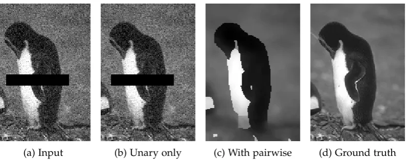
(a) Input (b) Unary only (c) With pairwise (d) Ground truth

Figure 2.3: An example of image inpainting with (c) and without (b) pairwise potentials. Note that the pairwise potentials ensure a smooth restoration.

the observed intensity. An example is [Szeliski et al., 2008],

θi(xi) =|I(i)−xi|2 , (2.6) where I(i) denotes the observed intensity at pixel i. Now, for this choice of unary term, if there is no pairwise term, then the restored image would be the same as the input (i.e., noisy). Usually the pairwise term is used as a smoothing cost which has the following form [Szeliski et al., 2008],

θij(xi,xj) =γijθ(|xi−xj|), (2.7) whereγij ≥0 is a weight depending on the pixelsiand jandθ(·)is a non-negative non-decreasing function. The function θ(·) is often referred to as the regularizer (or prior). A regularizer commonly used for this problem is,

θ(|xi−xj|) =min(|xi−xj|2,κ), (2.8) where κ is the maximum smoothness penalty. An image inpainting example with the energy formulation discussed above is shown in Figure 2.3.

2.1.1 Conditional Random Fields

Usually in computer vision applications we would like to use energy parameters that are data dependent. A probabilistic model which allows us to use data dependent energy parameters is the Conditional Random Field (CRF) [Lafferty et al., 2001]. A CRF can be defined as follows.

Definition 2.1.2. Consider two finite probability spaces: dataD, and labellingsΓ(e.g.,

P(x | d) is an MRF (as a distribution over x ∈ Γ), with the same neighbourhood structure for alld∈ D.

From an optimization point-of-view, the datadis given, and so the problem of op-timizingthe CRF means the task of optimizing the conditional probability distribution P(x | d), which is an MRF. In fact, apart from defining the probability distribution P(x|d), the data does not play any role in the optimization process. Therefore, from the optimization perspective both MRF and CRF models are identical and hence in this thesis, the term CRF refers to the corresponding MRF.

2.1.2 Optimizing an MRF

In general, optimizing an MRF may imply several meanings, such as finding the most probable assignment, computing the partition function or finding the marginal probabilities. In this thesis, we are interested in finding the most probable assignment or labelling of the MRF, and the term “optimizing an MRF” uniquely refers to this.

In most computer vision applications, we want to find an assignmentxthat max-imizes the probability. This is often referred to as the Maximum A Posteriori (MAP) estimation in the literature. Formally, it requires us to find the labellingx∗such that

x∗=argmax

x∈Ln

P(x), (2.9)

=argmax

x∈Ln 1

Zexp(−E(x)) ,

=argmin

x∈Ln

E(x).

The above simplification is due to the fact that the partition function is constant, and the exponential function is monotone. Now it becomes clear that, optimizing an MRF is equivalent to an energy minimizationproblem. Note that the minimization is over all possible assignments of x and the number of assignments is exponentially large. Therefore, this is an intractable (NP-hard) problem in general.

2.1.3 MRF Optimization Algorithms

et al., 2008] and has wide applicability in areas beyond computer vision and machine learning.

Even though, optimizing an MRF is NP-hard in general [Boykov et al., 2001], there are special cases (i.e., restricted classes of pairwise potentials and restricted graph structures) that can be solved optimally in polynomial time. In particular, if a binary MRF energy issubmodular(defined later in Definition 2.2.2), it is equivalent to a min-cut (sometimes called graph-cut) problem [Kolmogorov and Zabin, 2004] and there are many polynomial time algorithms to solve it [Ford and Fulkerson, 1962; Boykov and Kolmogorov, 2004]. Thissubmodularitycondition was later extended to multi-label MRFs [Schlesinger and Flach, 2006], hence such MRFs are solvable using a graph-cut algorithm [Ishikawa, 2003]. On the other hand, if the MRF is defined on a tree(an acyclic graph), then it can be solved using a message passing algorithm [Pearl, 1988].

Optimal algorithms are available only for certain restricted classes of MRFs and for general MRFs one has to settle with an approximate algorithm. The basic idea of designing an approximate algorithm is to utilize the optimal algorithms in some framework, such as in a move-making algorithm [Boykov et al., 2001] or a decomposition-based algorithm [Wainwright et al., 2005; Komodakis et al., 2011] in the continuous domain. In the former, the idea is to reduce the original MRF into a sequence of binary (or multi-label) submodular problems and solve them using a graph-cut al-gorithm. In the latter, the MRF is decomposed into optimally solvable subproblems (e.g., tree MRFs) and each subproblem is tackled independently. In most cases, the approximate algorithms provide a bound on their solution relative to the optimal solution.

The remainder of this chapter is dedicated to the state-of-the-art MRF optimiza-tion algorithms (both exact and approximate) and their basic theories are introduced in the relevant sections. In the next section, we discuss binary MRFs and their graph solvability. Next, we turn to the multi-label MRFs. In this section, we first review a graph-cut algorithm for multi-label submodular MRFs, and then formalize move-making algorithms and discuss useful special cases. Later, we consider the linear programming relaxation of the discrete problem. In this case, we will discuss a tree-based decomposition algorithm where each subproblem (tree MRF) is optimally minimized using the message passing algorithm. Finally, we briefly review other continuous relaxations based methods including the mean-field algorithm.

2

.

2

Binary MRF Optimization

Let us recall the energy function associated with a pairwise MRF (2.4), E(x) =

∑

i∈V

θi(xi) +

∑

(i,j)∈E

θij(xi,xj), (2.10)

and foreground-background segmentation. More than their applications, studying binary MRFs is important to understand the basic concepts of MRF optimization and to design move-making style approximate algorithms.

The idea is to formulate the minimization of the above energy function (2.10) as a min-cut problem and understand the required properties for it to begraph solvable, meaning it can be minimized optimally, using a graph-cut (or max-flow) algorithm in polynomial time [Ford and Fulkerson, 1962].

To this end, let us first introduce the concepts on pseuo-boolean optimization and submodular functions.

2.2.1 Pseudo-Boolean Functions

Definition 2.2.1. DefineB = {0, 1}. Apseudo-boolean functionis a mapping f :Bn _→ IR, where IR is the set of real numbers. Aquadratic pseudo-boolean functionis a pseudo-boolean function with maximum degree two.

Now, we will write the energy function (2.10) as a quadratic pseudo-boolean function. Note that the variablesxi ∈ B for alli∈ L. We denote the complement of xi with ¯xi,i.e., ¯xi =1−xi. This means ifxi =1, then ¯xi =0 and vice versa. With this notation, we can write Eq. (2.10) as

E(x) =

∑

i∈V

(θi:0x¯i+θi:1xi) +

∑

(i,j)∈E

θij:00x¯ix¯j+θij:01x¯ixj+θij:10xix¯j+θij:11xixj

. (2.11) Here, we use the shorthandθi:λ =θi(λ)andθij:λµ =θij(λ,µ). It is clear that Eq. (2.11)

is a quadratic pseudo-boolean function.

In general minimizing a quadratic pseudo-boolean function is an NP-hard prob-lem [Boros and Hammer, 2002], meaning that there does not exist a polynomial time algorithm for finding the minimum (unless P = NP). However, we will now see a useful special case, where an efficient polynomial time algorithm can be used to find the minimum.

2.2.2 Submodular Functions

The submodularity condition is usually defined on set functions [Fujishige, 2005]. However, due to the one-to-one correspondence between set functions and pseudo-boolean functions, one can define it as follows.

Definition 2.2.2. A pseudo-boolean function f :Bn _{→IR issubmodular if}

f(x) + f(y)≥ f(x∨y) + f(x∧y), (2.12) for allx,y∈ Bn_{. Here∨and∧are componentwise logical OR and AND operations.} For a quadratic pseudo-boolean function with n = 2, the submodularity definition reduces to

Now, it is easy to see that the energy function (2.11) is submodular if the pairwise terms satisfy the following inequality

θij:01+θij:10≥ θij:00+θij:11 , (2.14) for all(i,j)∈ E. Note that there is no condition on the unary potentials and hence, they can be arbitrary.

Example 2.2.1. Consider a binary segmentation problem where foreground is de-noted with label 1 and background with label 0. Here the unary potentials are based on the image intensities and possibly learned from the dataset. To have a smooth segmentation, the pairwise potentials usually have the following form (see Exam-ple 2.1.1),

θ_ij(x_i,x_j) =γ_ijθ(|x_i−x_j|), (2.15) whereγij ≥0 is a weight depending on the pixelsiand jandθ(·)is a non-negative non-decreasing function. For an MRF with binary labels,

θ_ij:00=θ_ij:11=γ_ijθ(0), (2.16) θij:01=θij:10=γijθ(1),

whereθ(0)≤ θ(1). Therefore, from Eq. (2.14), such an MRF is submodular. Further-more, these pairwise potentials are often referred to asattractive potentials.

The significance of submodularity is that, such an energy function is graph solv-able. Let us now discuss the graph representability of quadratic pseudo-boolean functions and then turn to the max-flow algorithm.

2.2.3 Graph Representability

In this section, we discuss how a quadratic pseudo-boolean function can be repre-sented by anst-graph.

Definition 2.2.3. An st-graph is a weighted directed graph ˆG = (V ∪ {0, 1}, ˆˆ E+_,

φ).

Here ˆV is the set of vertices or nodes and {0, 1} are special nodes2, called source and terminal respectively. Here ˆE+ _{is the set of directed edges and the undirected}

edges are denoted with ˆE, where(i,j) ∈ Eˆ means (i,j) ∈ Eˆ+ _{and(j,i) ∈ Eˆ}+_{. The}

set of edge weights (or capacities) are denoted with φ, which has a real value φij for each directed edge (i,j) ∈ Eˆ+_{. Furthermore, we introduce notations ˆE}

e and ˆEι,

where ˆE = Eˆ_e∪Eˆ_ι, to denote theexternaledges (i.e., those connecting the source or the terminal) and theinternaledges (i.e., ˆE_ι ⊂V ׈ Vˆ).

Definition 2.2.4. Apartition or cutof an st-graph is a division of the vertices ˆV into two disjoint subsets ˆV₀and ˆV₁, such that 0∈Vˆ₀and 1∈Vˆ₁. The cost of the partition

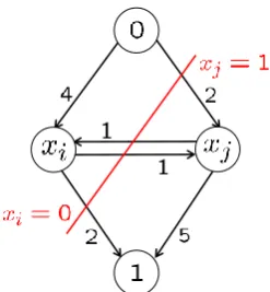
Figure 2.4: Example of an st-graph. Here, the cut({xi},{xj})corresponds to the labelling x= {0, 1}and the cost of the cut is CGˆ({xi},{xj}) =2+1+2=5.

is the sum of weights on the edges passing from ˆV0 to ˆV1,

CGˆ(Vˆ0, ˆV1) =

∑

i∈Vˆ0,j∈Vˆ1

φij . (2.17)

Example of anst-graph is shown in Figure 2.4. Anst-graph represents the binary labelling in a different way. In fact, each labelling x is determined by the partition

(Vˆ₀, ˆV₁), specifically, xi = 1 if and only if i ∈ Vˆ1. Then the function value for any labelling is equal to the cost of the corresponding partition,

f(x) =CGˆ(Vˆ0, ˆV1). (2.18)

Consider an edge(i,j)∈Eˆ+_{such thati∈Vˆ}

0andj∈Vˆ1. This edge contributes to the cost of the partition for the labelling xi = 0 and xj = 1. Therefore, an edge (i,j) in thest-graph represents the termφijx¯ixj. Similarly, the edges from the source (node 0) and the edges to the terminal (node 1) represent the linear terms. In particular, for alli∈ Vˆ,

φ0i ¯0xi = φ0ixi edge 0→i, (2.19) φi1x¯i1= φi1x¯i edgei→1 ,

φ01¯0 1 = φ01 edge 0→1 .

Note that the constant term is represented by an edge 0 → 1. Now, we can write the quadratic pseudo-boolean function represented by an st-graph in the following form,

f(x) =φ01+

∑

i∈Vˆ

(φ0ixi+φi1x¯i) +

∑

(i,j)∈Eˆ+

ι

φijx¯ixj . (2.20)

Eq. (2.20) can be reparametrized (using the identity ¯xi = 1−xi) to make the coeffi-cients of the linear terms non-negative. In particular, for all i ∈ Vˆ, φ0i,φi1 ≥ 0 and φ01may be negative. However, the constant term does not play any role in the mini-mization and hence it can be removed from the graph. For the quadratic terms, this reparametrization trick do not make any coefficients non-negative and they need to be non-negative to start with. Let us state it as a theorem.

Theorem 2.2.1. Let f(x)be a quadratic pseudo-boolean function represented by an st-graph as in Eq.(2.20). Ifφij ≥0for all(i,j)∈Eˆι+, thenminx f(x)can be obtained in polynomial

time.

Proof. This is the standard result of graph solvability of quadratic pseudo-boolean functions. See [Ford and Fulkerson, 1962; Boros and Hammer, 2002].

2.2.3.1 Representing the Binary MRF Energy in an st-graph

We now discuss how one can represent the energy function (2.11) in an st-graph. To this end, the set of vertices V and the set of edges E of the MRF graph have one-to-one correspondence with the set ˆV and ˆEι of thest-graph. Specifically,

ˆ

V =V , (2.21)

ˆ Eι =E .

Additionally, there are external edges in thest-graph connecting the vertices ˆV with the source and the terminal nodes. Now, it remains to find the edge capacities that would represent the energy function exactly for all label assignments.

Let us now rewrite the energy function (2.11) in the form of Eq. (2.20). This can be done using the identity ¯xi =1−xi for alli∈ V.

E(x) =

∑

i∈V

(θi:0x¯i+θi:1xi) +

∑

(i,j)∈E

θij:00x¯ix¯j+θij:01x¯ixj+θij:10xix¯j+θij:11xixj

,

(2.22)

=

∑

i∈V

(θi:0x¯i+θi:1xi) +

∑

(i,j)∈E

θij:00x¯i+θij:10xi+ (θij:11−θij:10)xj

+

∑

(i,j)∈E

(θij:01+θij:10−θij:00−θij:11)x¯ixj .

The edge capacities φ can be easily derived from the above equation. An st-graph

representation of a unary term and a pairwise term are shown in Figure 2.5.

From Theorem 2.2.1, to minimize this energy function optimally, the coefficients of the quadratic terms need to be non-negative. Note that, for a submodular quadratic pseudo-boolean function,

mini-Figure 2.5: The st-graph representation of a binary MRF energy function. Specifically, the unary term (left) for the node i∈ V and the pairwise term (right) for the edge(i,j)∈ E are represented in the st-graph, for the energy function(2.22).

mum energy labelling can be obtained in polynomial time using a min-cut algorithm in the correspondingst-graph.

2.2.4 Min-Cut and Max-Flow

In this section, we establish the connection between the min-cut and max-flow prob-lems. To this end, let us first define a flow in anst-graph as follows.

Definition 2.2.5. Given an st-graph ˆG = (V ∪ {0, 1}, ˆˆ E+_,

φ), a flow is a mapping ψ : ˆE+ → IR, denoted byψij for the edge(i,j) ∈ Eˆ+, that satisfies the anti-symmetry condition ψ_ij = −ψ_ji for all (i,j) ∈ E. A flow is calledˆ conservative3 if the total flow into a node is zero for all nodes except for the source and the terminal, i.e., for all i∈Vˆ,

∑

(j,i)∈Eˆ+

ψji=0 . (2.24)

Once a flow ψis passed in anst-graph, the edge capacitiesφare updated as,

φ0 =φ−ψ, (2.25)

whereφ0 are called theresidualcapacities.

Definition 2.2.6. A flowψis calledpermissibleifφij−ψij ≥0 for all(i,j)∈Eˆ+. Note that, if a permissible flow is passed in anst-graph with non-negative capac-ities, then the capacities remain non-negative.

As we have seen in the previous section, finding the minimum of a submodular quadratic pseudo-boolean function is the same as finding the min-cut solution of the correspondingst-graph. This can be achieved by finding the maximum flow (shortly

max-flow) from the source (0 node) to the terminal (1 node). In fact, min-cut and max-flow are dual LP problems. We now state the well-known min-cut/max-flow theorem [Ford and Fulkerson, 1962] below.

Theorem 2.2.2. Consider a submodular quadratic pseudo-boolean function f(x)and let ψ

be a permissible conservative flow on the corresponding st-graph. Then,

min

x f(x) =maxψ

∑

(0,i)∈Eˆ+

ψ0i . (2.26)

Proof. This is a result of the duality between the max-flow and min-cut problems and can be proven by computing the Lagrange dual of one of them. See [Ford and Fulkerson, 1962].

Max-Flow Algorithms. Broadly speaking, there are three different kinds of max-flow algorithms: those relying on finding augmenting paths [Ford and Fulkerson, 1962], the push-relabel approach [Goldberg and Tarjan, 1988] and the pseudo-flow techniques [Chandran and Hochbaum, 2009]. The polynomial time guarantee of max-flow was first proven in [Edmonds and Karp, 1972] by modifying the augment-ing path algorithm, to always find theshortestaugmenting path. There are numerous max-flow implementations available for general purpose as well as specific to com-puter vision applications. Among them, the specialized implementations are signif-icantly faster in practice. In particular, the BK method [Boykov and Kolmogorov, 2004] is arguably the fastest implementation for 2D and sparse 3D graphs arising from computer vision applications. Recently, for dense problems, the EIBFS algo-rithm [Goldberg et al., 2015] was shown to outperform the BK method.

2.2.5 Non-Submodular MRFs

Non-submodular MRF energy functions can also be represented by anst-graph, but the graph would contain negative edges. Therefore the standard max-flow tech-niques cannot be applied. However, such an energy function can be approximated using a roof-dual technique [Boros and Hammer, 2002]. Such a technique is usually known as Quadratic Pseudo-Boolean Optimization (QPBO) and it can be used to ob-tain a partially optimal labelling. In other words, the optimal labels can be obob-tained only for a subset of nodes and the unlabelled nodes are usually assigned based on some heuristics. We refer the interested reader to [Boros and Hammer, 2002] for a detailed treatment on pseudo-boolean optimization.

2

.

3

Multi-Label MRF Optimization

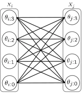
Figure 2.6: Example of a multi-label graph. Here the nodes represent the unary potentials θi:λand the edges represent the pairwise potentialsθij:λµ.

2.3.1 Multi-Label Graph

An alternative way of representing an MRF labellingx ∈ Ln _{is by definingindicator} variables xi:λ ∈ {0, 1}, where xi:λ = 1 if and only if xi = λ. For a given i, exactly

one of xi:λ;λ ∈ Lcan have value 1. In terms of the indicator variables, the energy

function (2.4) may be written as E(x) =

∑

i∈Vλ

∑

θi:λxi:λ+

∑

(i,j)∈Eλ,

∑

θij:λµxi:λxj:µ . (2.27)

Here, we use the shorthand θi:λ = θi(λ) and θij:λµ = θij(λ,µ). One may define a

graph, called amulti-label graph, with nodes denoted byXi:λ;i∈ V, λ∈ L, as shown

in Figure 2.6. This graph represents the energy function. Given a labelling x, the value of the energy function is obtained by summing the weights on all nodes with xi:λ =1 (in other wordsxi = λ) plus the weightsθij:λµsuch thatxi:λ =1 andxj:µ =1.

This multi-label graph representation of the energy function (2.27) will be useful to understand some properties of the energy as well as the algorithms used to minimize it.

2.3.2 Ishikawa Algorithm

Ishikawa [Ishikawa, 2003] introduced a method to solve (minimize the energy) of multi-label MRFs with convex edge terms. This method can be easily extended [Schlesinger and Flach, 2006] to energy functions satisfying a multi-label submodu-larity condition, analogous to the submodularity condition for MRFs with binary labels.

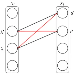
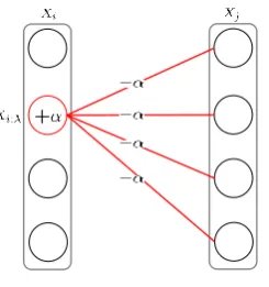
de-Figure 2.7: The multi-label submodularity condition illustrated using the multi-label graph. The sum of red edge capacities must be greater than or equal to the sum of black edge capacities.

fined below.

Definition 2.3.1. The energy function given in Eq. (2.27) is multi-label submodular if the pairwise potentials satisfy

θij:λ0µ+θij:λµ0−θij:λµ−θij:λ0µ0 ≥0 , (2.28)

for allλ<λ0 andµ<µ0. This condition assumes an ordered label set.

Note that the multi-label submodularity condition (2.28) can be equivalently stated as,

θij:λ+1µ+θij:λµ+1−θij:λµ−θij:λ+1µ+1 ≥0 , (2.29) forλ,µ∈ {0, . . .`−2}. This can be easily verified using induction. Figure 2.7 shows this condition graphically, in the multi-label graph.

Example 2.3.1. Consider pairwise potentials of the form,

θij:λµ= γijθ(|λ−µ|), (2.30)

where γij ≥ 0 and θ(·) is a convex function4. Substituting this in Eq. (2.29) and neglectingγij,

θ(|λ−µ+1|) +θ(|λ−µ−1|)−2θ(|λ−µ|)≥0 . (2.31) This is true for a convex function θ(·). These pairwise potentials are referred to as convex priors and they constitute a multi-label submodular energy function. See Figure 2.8 for some examples of convex priors used in computer vision.

Ishikawa [Ishikawa, 2003] introduced a different way of representing the multi-label energy function. The basic idea behind the Ishikawa construction is to encode the label Xi = xi of a vertexi ∈ V using binary-valued random variables Ui:λ, one

4_{A function f :X →IR isconvexif for allx,y∈ X andt∈[0, 1], f(t x+ (1−t)y)≤t f(x) + (1−}

(a) Quadratic (b) Linear (c) Huber

Figure 2.8: Examples of convex priors:a)θ(|δ|)is a quadratic function;b)a linear function; andc)a Huber function (Eq.(2.43)).

for each labelλ ∈ L. In particular, the encoding is defined asui:λ = 1 if and only if

xi ≥λ, and 0 otherwise. The Ishikawa graph is then anst-graph (see Definition 2.2.3) ˆ

G = (V ∪ {0, 1}, ˆˆ E+_,

φ), where the set of nodes and the set of edges are defined as

follows,

ˆ

V ={U_i:λ |i∈ V,λ∈ {1,· · · ,`−1}}, (2.32)

ˆ

E+ =Eˆ_v+∪Eˆ_c+, ˆ

E_v+ ={(Ui:λ,Ui:λ±1)|i∈ V,λ∈ {1,· · · ,`−1}} ,

ˆ E+

c ={(Ui:λ,Uj:µ),(Uj:µ,Ui:λ)|(i,j)∈ E,Ui:λ,Uj:µ∈ V }ˆ ,

where ˆE+

v is the set of vertical edges and ˆEc+ is the set of cross edges. Note that the directed edges are denoted with +_{. We denote the Ishikawa edges by e}

ij:λµ ∈ Eˆ+

and their capacities byφij:λµ. We also denote byei:λthe downward edge(Ui:λ+1,Ui:λ).

An example of an Ishikawa graph is shown in Figure 2.9. From the definition ofU_i:λabove, we find the basic relation

xi:λ =ui:λ−ui:λ+1 , (2.33)

=u¯i:λ+1−u¯i:λ ,

=u¯i:λ+1ui:λ ,

which also entails the relation ui:λ ≥ ui:λ+1. In addition, since xi ≥ 0, it follows

that ui:0 = 1. Thus, node Ui:0 is identified with the vertex 1. Furthermore, since

xi < `, we may identify ui:` = 0. In other words, nodes Ui:0 may be identified with node 1 andU_i:` with node 0, which is useful in interpreting Eq. (2.33) for allλ∈ L . Consequently, only the nodesUi:λforλ∈ {1,· · · ,`−1}are included in the set ˆV.

In an st-graph, a labeling x is represented by a cut (see Definition 2.2.4) in the graph. Therefore, in the Ishikawa graph, if the downward edgeei:λ is in thecut, then

vertex i takes labelλ. In MRF energy minimization, each vertex itakes exactly one labelxi, which means that exactly one edgeei:λmust be in the min-cut of the Ishikawa

graph. This is ensured by having infinite capacity for each upward edgeeii:λλ+1,i.e.,

φii:λλ+1 =∞for alli∈ Vandλ∈ L. Since the energy of a labelling is represented by

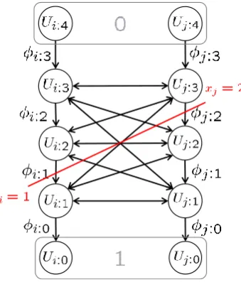
Figure 2.9: Example of an Ishikawa graph. The graph incorporates edges with infinite ca-pacity from Ui:λ to Ui:λ+1, not shown in the graph. Here the cut corresponds to the labeling

x= {1, 2}where the label setL= {0, 1, 2, 3}.

as follows,

θi:λ =φii:λ+1λ =φi:λ , (2.34)

θij:λµ=

∑

φij:λ0µ0+

∑

φji:µ0λ0 .

Now, we need to determine the capacities φ from the energy parametersθ. To this

end, one can work out how an energy function of the form (2.27) may be written in terms of the variables ui:λ, and hence encoded in an Ishikawa graph. Given the

energy function (2.27), one wishes to write it in the form representable by anst-graph (see Section 2.2.3),

E(x) =φ01+

∑

i∈V

λ∈L

φi:λu¯i:λ+1ui:λ+

∑

(i,j)∈E

λ,µ∈L

φij:λµu¯i:λuj:µ. (2.35)

To this end, we substitutexi:λ =u¯i:λ+1ui:λ and

x_i:λxj:µ= (u¯i:λ+1−u¯i:λ) (uj:µ−uj:µ+1), (2.36) = u¯i:λ+1uj:µ+u¯i:λuj:µ+1−u¯i:λuj:µ−u¯i:λ+1uj:µ+1,