A time discretisation scheme based on integrated radial
basis functions for heat transfer and fluid flow problems
T.T.V. Le
a, N. Mai-Duy
a,∗, K. Le-Cao
band T. Tran-Cong
a aComputational Engineering and Science Research Centre,
School of Mechanical and Electrical Engineering,
University of Southern Queensland, Toowoomba, QLD 4350, Australia
bDepartment of Mechanical Engineering, Faculty of Engineering,
National University of Singapore, Singapore
Submitted to
Numerical Heat Transfer, Part B
, April/2018; revised,
August/2018
Short title: An integrated-RBF-based time discretisation scheme
ABSTRACTThis paper reports a new numerical procedure, which is based on integrated radial
basis functions (IRBFs) and Cartesian grids, for solving time-dependent differential problems that
can be defined on non-rectangular domains. For space discretisations, compact five-point IRBF
stencils [Journal of Computational Physics, vol. 235, pp. 302-321, 2013] are utilised. For time
discretisations, a two-point IRBF scheme is proposed, where the time derivative is approximated
in terms of not only nodal function values at the current and previous time levels but also nodal
derivative values at the previous time level. This allows functions other than a linear one to also
be captured well on a time step. The use of the RBF width as an additional parameter to enhance
the approximation quality with respect to time is also explored. Various kinds of test problems of
heat transfer and fluid flows are conducted to demonstrate attractiveness of the present compact
approximations.
Keywords: time discretisations; integrated radial basis functions; compact approximations; heat
transfer and fluid flows.
NOMENCLATURE
c integration constant t time variable
CM convergence measure T temperature
D side length of outer square cylinder u, v x and y components of velocity
Di diameter of inner cylinder w RBF weight
g gravitational acceleration W width of rectangular channel
G radial basis function (RBF) x spatial variable
h water depth x, y coordinates
H mean water depth β thermal expansion coefficient
I/Q spatial/temporal integrated RBF βs spatial RBF width
k time level βt temporal RBF width
l thermal conductivity γ thermal diffusivity
L length of rectangular channel ǫ tolerance
m number of RBFs/nodal points ζ water surface elevation
MAE maximum of absolute error ν kinematic viscosity
n normal direction ψ stream function
nip number of interior points ω vorticity
nt total number of time steps Subscripts
Ne discrete relative L2 error b boundary value
Nu Nusselt number [α] a component ofx
P r Prandtl number Superscripts
Ra Rayleigh number e exact solution
RMSE root-mean-square error (q) order of an IRBF scheme
1
Introduction
Over the last twenty five years, radial basis functions (RBFs), which possess the property of
universal approximation, have been used with great success to solve different types of differential
set of unstructured discrete points and they have the ability to produce highly accurate results.
Approximations of the field variable and its derivatives in terms of RBFs can be constructed
through the differential process (DRBF) [4] or the integral process (IRBF) [5]. The latter was
originally developed to (i) avoid the reduction in convergence rate caused by differentiation; and (ii)
provide an effective way of implementing multiple boundary conditions. For global RBF methods,
a function is approximated using all RBFs over the domain. It is known that the global RBF
system matrix is fully populated and its condition number grows rapidly with increasing number
of nodes. To circumvent this problem, there have been several attempts in the development of
local RBF methods, where only a small subregion, namely the influence domain, is activated for
the construction of the RBF approximations at a point. Works reported include [6-14]. Local
methods lead to a sparse and better-conditioned system matrix. However, their solution accuracy
is observed to significantly deteriorate. Compact local RBF methods have been developed. In
these methods, the approximations involve nodal values of not only the field variable but also its
derivatives [10,15,16], which allows both a high level of the solution accuracy and sparseness of
the system matrix to be achieved together. In using RBFs to solve differential problems, the time
derivative terms are usually discretised by means of low-order finite differences (FDs), for which
small time steps are typically required. In this study, we propose a discretisation procedure based
on compact IRBF stencils only for time-dependent heat and fluid flow problems in two dimensions.
An IRBF stencil is of 2 nodes and 5 nodes for time and space discretisations, respectively.
The remainder of the paper is organised as follows. Section 2 gives a brief review of integrated
RBFs and their compact forms for space discretisations. Section 3 describes a new compact
two-point approximation based on IRBFs for time discretisations, and a numerical procedure based on
compact IRBF stencils only for solving time-dependent differential problems. Numerical results
2
Integrated RBFs
Our proposed numerical procedure is based on integrated RBFs. Some relevant schemes of IRBFs
are briefly reviewed here for the sake of completeness.
2.1
Original scheme
Highest-order derivatives of the field variable f in the ordinary/partial differential equations
(ODEs/PDEs) are decomposed into RBFs, from which expressions for lower-order derivatives
and the variable itself are derived through integration
∂qf(x)
∂αq = m
X
i=1
w[α]iGi(x) = m
X
i=1
w[α]iI
(q)
[α]i(x), (1)
∂q−1f(x)
∂αq−1 =
m
X
i=1
w[α]iI
(q−1)
[α]i (x) +c[α]1, (2)
. . . .
f(x) =
m
X
i=1
w[α]iI[(0)α]i(x) +
αq−1
(q−1)!c[α]1+
αq−2
(q−2)!c[α]2+...+c[α]q, (3)
where α is a component of the independent spatial variable x, the subscript [α] is used to
dif-ferentiate the IRBF approximations with respect to each coordinate, m the number of RBFs,
Gi(x) the RBF, I( q−1)
[α]i (x) =
R
I[(αq)]i(x)dα, ...,I
(0)
[α]i(x) =
R
I[(1)α]i(x)dα, (w[α]1, w[α]2, ..., w[α]m) the
coefficients, and (c[α]1, c[α]2, ..., c[α]q) the integration constants that are functions of variables other
than α. Making use of (1)-(3) and point collocation, one can transform the ODE/PDE into a set
2.2
Compact approximation scheme
IRBFs have been used to construct the approximations on Cartesian grids representing a domain
of rectangular/non-rectangular shape [1,17]. Advantages of this approach lie in its economic
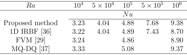
preprocessing. Consider a domain that is embedded in a Cartesian grid as shown in Figure 1. Grid
points outside the domain (external points) together with the internal points that fall very close
-within a small distance - to the boundary are removed. The remaining grid points are taken to be
the interior nodes. The boundary nodes are points that are generated by the intersection of the
grid lines with the boundaries. In this work, second order differential problems are considered and
for a space discretisation, a 5-point stencil associated with node (i, j) is employed with nodes being
locally numbered from left to right and from bottom to top ((i, j) ≡ 3) (Figure 1). Derivatives of the dependent variablef in thex and y directions are approximated by IRBFs along the lines
defined by 1−3−5 and 2−3−4, respectively. One can utilise the integration constants in the IRBF formulation to incorporate some nodal derivative values in the approximations. In the x
direction, evaluation of (3) at (x1, x3, x5) and of (1) at (x1, x5) using q= 2 result in
e f = " I B #
| {z }
C
e
w, (4)
where
e
f = f1 f3 f5 ∂
2 f1 ∂x2 ∂2 f5 ∂x2 T , (5) e
w= w[x]1 w[x]3 w[x]5 c[x]1 c[x]2
T , (6) I =
I[(0)x]1(x1) I (0)
[x]3(x1) I (0)
[x]5(x1) x1 1
I[(0)x]1(x3) I (0)
[x]3(x3) I (0)
[x]5(x3) x3 1
I[(0)x]1(x5) I[(0)x]3(x5) I[(0)x]5(x5) x5 1
and
B=
"
I[(2)x]1(x1) I (2)
[x]3(x1) I (2)
[x]5(x1) 0 0
I[(2)x]1(x5) I (2)
[x]3(x5) I (2)
[x]5(x5) 0 0
#
.
The system (4) can be solved for the unknown coefficient vector we, resulting in
e
w=C−1f ,e (7)
where C−1 is the inverse of C.
Expressions for computing f and its derivatives at point x, where x1 ≤ x ≤ x5, can then be
obtained by substituting (7) into (3), (2) and (1) with q= 2
f(x) =h I[(0)x]1(x) I[(0)x]3(x) I[(0)x]5(x) x 1 iC−1f ,e (8)
∂f(x)
∂x =
h
I[(1)x]1(x) I (1)
[x]3(x) I (1)
[x]5(x) 1 0
i
C−1f ,e (9)
∂2f(x)
∂x2 =
h
I[(2)x]1(x) I (2)
[x]3(x) I (2)
[x]5(x) 0 0
i
C−1f ,e (10)
which can be rewritten as
f(x) =φ1(x)f1+φ3(x)f3+φ5(x)f5+ ¯φ1(x)
∂2f 1
∂x2 + ¯φ5(x)
∂2f 5
∂x2 , (11)
∂f(x)
∂x =
dφ1(x)
dx f1+
dφ3(x)
dx f3+
dφ5(x)
dx f5+
dφ¯1(x)
dx ∂2f
1
∂x2 +
dφ¯5(x)
dx ∂2f
5
∂x2 , (12)
∂2f(x)
∂x2 =
d2φ 1(x)
dx2 f1 +
d2φ 3(x)
dx2 f3+
d2φ 5(x)
dx2 f5+
d2φ¯ 1(x)
dx2
∂2f 1
∂x2 +
d2φ¯ 5(x)
dx2
∂2f 5
At x=x3, they reduce to
∂f3
∂x =µ1f1+µ3f3+µ5f5+ ¯µ1 ∂2f
1
∂x2 + ¯µ5
∂2f 5
∂x2 , (14)
∂2f 3
∂x2 =η1f1+η3f3+η5f5 + ¯η1
∂2f 1
∂x2 + ¯η5
∂2f 5
∂x2 , (15)
whereµ1 =dφ1(x3)/dx,µ3 =dφ3(x3)/dx,µ5 =dφ5(x3)/dx, ¯µ1 =dφ¯1(x3)
dx, ¯µ5 =dφ¯5(x3)
dx,
η1 = d2φ1(x3)/dx2, η3 = d2φ3(x3)/dx2, η5 = d2φ5(x3)/dx2, ¯η1 = d2φ¯1(x3)
dx2, and ¯η 5 =
d2φ¯ 5(x3)
dx2.
Similarly, on the line 2−3−4, one obtains
∂f3
∂y =ν2f2+ν3f3+ν4f4+ ¯ν2 ∂2f
2
∂y2 + ¯ν4
∂2f 4
∂y2 , (16)
∂2f 3
∂y2 =θ2f2 +θ3f3+θ4f4+ ¯θ2
∂2f 2
∂y2 + ¯θ4
∂2f 4
∂y2 . (17)
With nodal derivative values being approximated in the form of (14), (15), (16) and (17),
collo-cating the ODE/PDE at grid nodes will lead to a sparse system matrix, of which each row has
only 5 entries. Note that the nodal derivative values on the right hand side of (14)-(17) can be
treated as known quantities.
3
Proposed IRBF-based method
3.1
An IRBF-based two-point time discretisation scheme
In the proposed scheme, the variation of the dependent variable f on each interval (time step)
the following parabolic PDE
∂f
∂t (x, y, t)−
∂2f
∂x2 (x, y, t) +
∂2f
∂y2 (x, y, t)
=b(x, y, t), (18)
defined on the domain Ω and subjected to initial values and boundary conditions. In (18), b is a
given function (the source). Using the conventional finite difference method, one can reduce the
PDE to
fk ij −f
k−1
ij
∆t −λ
∂2fk ij
∂x2 +
∂2fk ij
∂y2
!
−(1−λ) ∂
2fk−1
ij
∂x2 +
∂2fk−1
ij
∂y2
!
=bk−1+λ
ij , (19)
where the subscript ij is used to denote the function at grid node (i, j), the superscript k the
function evaluated at the time level tk, ∆t = tk −tk−1, and λ = 0 and λ = 1 correspond to
the explicit and implicit schemes, respectively. Our goal here is to construct an approximating
function from RBFs, which can capture a curved line rather than a straight line over two nodes
tk−1 and tk. It is proposed that the first-order derivative off with respect to t is decomposed into
RBFs
∂f(t)
∂t =wk−1Gk−1(t) +wkGk(t), (20)
where, for the multiquadric (MQ) case,Gk−1(t) = q
(t−tk−1)
2+a2
k−1andGk(t) = p
(t−tk)2+a2k
in which ak−1 and ak are the MQ widths. Expression for computing f is then derived as
f(t) =wk−1Qk−1(t) +wkQk(t) +c1, (21)
whereQk−1(t) = R
Gk−1(t)dt,Qk(t) = R
Gk(t)dt, andc1 is the constant of integration. It should
be emphasised that functionf in (21) is defined with three coefficients (i.e. wk−1,wk andc1) over
two nodal points (i.e. tk−1 and tk). This allows one to add one extra equation in the system of
derivative value of f evaluated at the previous time level. Its details are as follows
fk
fk−1
∂f ∂t
k−1
=Ct
wk−1
wk
c1
, (22)
where Ct is the conversion matrix defined as
Ct=
Qk−1(tk) Qk(tk) 1
Qk−1(tk−1) Qk(tk−1) 1
Gk−1(tk−1) Gk(tk−1) 0
.
Making use of (22), the three coefficients can be expressed in terms of the nodal variable values
and the derivative value at the previous time level
wk−1
wk
c1
=C−1
t
fk
fk−1
∂f ∂t
k−1
. (23)
Expression for computing the first-order derivative at the current time level thus becomes
∂f ∂t
k
=h Gk−1(tk) Gk(tk) 0 i
wk−1
wk
c1
, (24)
=h Gk−1(tk) Gk(tk) 0 i
Ct−1
fk
fk−1
∂f ∂t
k−1
, (25)
which can be rewritten as
∂f ∂t
k
=D1fk+D2fk−1+D3f˙k−1, (26)
with D1, D2, D3 being computed from the RBFs and the inverse of Ct - they are known values.
The time derivative term is now expressed in term of values off attk−1 and tk (i.e. f
k−1 and fk)
and its time derivative at tk−1 (i.e.
∂f ∂t
k−1
scheme (19) is
D1fijk+D2fijk−1+D3f˙ijk−1−λ
∂2f
ij ∂x2 k +∂ 2f ij ∂y2 k!
−(1−λ) ∂
2f
ij
∂x2
k−1
+∂
2f
ij
∂y2
k−1!
=bk−1+λ
ij .
(27)
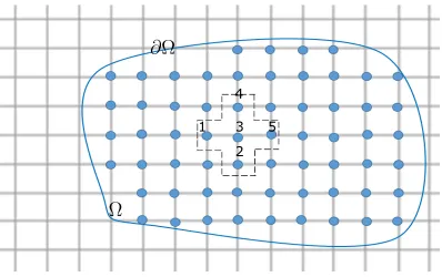
As shown in Figure 2, a function approximated by IRBFs on a time step can be of nonlinear
form. It is expected that larger time steps can be used in simulating time-dependent differential
problems, where the slope of the solution varies between time levels.
3.2
An IRBF-based space-time discretisation scheme
The combination of the proposed compact 2-point stencil for time and the presented compact
5-point stencil for space results in a numerical procedure, which is based on IRBFs only, for solving
time-dependent differential problems. With the explicit scheme (i.e. λ = 0), the calculation is
based on the solution of (15) and (17) evaluated at the previous time level
−η¯1
∂2f 1
∂x2
k−1
+∂
2f 3
∂x2
k−1
−η¯5
∂2f 5
∂x2
k−1
=η1f1k−1+η3f3k−1+η5f5k−1, (28)
−θ¯2
∂2f 2
∂y2
k−1
+ ∂
2f 3
∂y2
k−1
−θ¯4
∂2f 4
∂y2
k−1
=θ2f2k−1+θ3f3k−1+θ4f4k−1. (29)
It can be seen that these two equations for nodal derivative values lead to systems of tridiagonal
algebraic equations on thexandygrid lines that can be solved efficiently by the Thomas algorithm.
Note that nodal values of second derivatives on the boundary can be calculated using any 1D
approximation scheme on their associated grid lines. In some cases such as rectangular domains,
instead of using 1D approximations, one can directly derive these values from the governing
equation and the given boundary conditions.
values off and its second derivatives in thexandydirections). A set of three algebraic equations
needed for each node consists of the two equations (15) and (17) evaluated at the current time
level, i.e.
−η¯1
∂2f 1 ∂x2 k + ∂ 2f 3 ∂x2 k
−η¯5
∂2f 5
∂x2
k
=η1f1k+η3f3k+η5f5k, (30)
−θ¯2
∂2f 2 ∂y2 k +∂ 2f 3 ∂y2 k
−θ¯4
∂2f 4
∂y2
k
=θ2f2k+θ3f3k+θ4f4k. (31)
and the equation directly derived from the PDE (i.e. equation (27)). It is possible to combine
these three equations to form two tridiagonal algebraic equations through the implicit elimination
approach as discussed in [1].
4
Numerical examples
In this study, IRBFs are implemented with the multiquadric (MQ) function in the form of
Gi(α) =
q
(α−ci)2+a2i, (32)
where ci and ai are the centre and the width of the ith MQ, respectively and α can be x or y in
the spatial approximation and t in the temporal approximation. The MQ width is simply chosen
according to the relation
ai =βsdi for space, (33)
ai =βt∆t for time, (34)
where βs and βt are positive values, di the smallest distance between the centre ci and its
neigh-bours, and ∆t the time step. Different types of time-dependent problems are chosen to study the
the heat transfer, convection-diffusion and shallow water equations, of which the analytic solutions
are available. In the fourth (last) example, the proposed method is applied for the simulation of
natural convection flows in the region between a square outer cylinder and a circular inner
cylin-der. Some standard finite difference schemes are also employed where appropriate to provide the
base for the evaluation of accuracy of the proposed time stencil. Note that a distinguishing feature
of the RBF solution is that its accuracy can be controlled not only by the grid size/time step but
also by the RBF width. For all numerical examples, the problem domain is simply discretised
using a uniform Cartesian grid. The value of di in (33) thus becomes a grid size. In the case of
curved boundaries, a distance to the boundary used for the removing of interior nodes is chosen
asdi/8. When the analytic solution is available, the numerical error is measured in the form of
1. Discrete relative L2 norm
Ne=
pPm
i=1(fie−fi)2
pPm
i=1(fie)2
, (35)
2. Root-mean-square error (RMSE)
RMSE =
v u u
t 1
nt nt
X
i=1
(fe
i −fi)2, (36)
3. Maximum of absolute error (MAE)
MAE =kfie−fikmax, (37)
where m is the number of nodal points, nt the number of time steps, and fe and f respectively
denote the exact and approximate solutions. In the last example, the flow is considered to reach
the steady state when the following condition is satisfied
CM =
qPnip
i=1 fik−f k−1
i
2
qPnip
i=1 fik
where nip is the number of interior points, k the time level, f the stream function and ǫ the
tolerance. In this study, ǫ is taken to be 10−12.
4.1
Example 1: Parabolic PDEs
4.1.1 One dimensional space
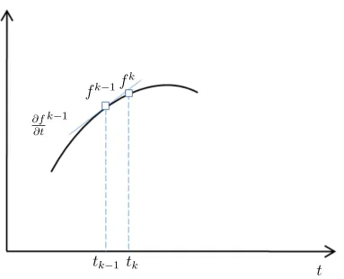
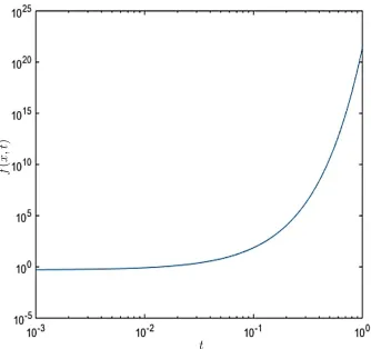
The proposed method is first verified in the following PDE
∂f
∂t (x, t) = ∂2f
∂2x(x, t) +b(x, t), 0≤x≤1, (39)
with b(x, t) = 50xe50t. Its exact solution is given by
fe(x, y, t) =xe50t, (40)
from which one can derive the initial values and Dirichlet boundary conditions. As shown in
Figure 3, functionf grows very quickly with time.
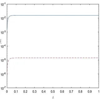
To assess accuracy of the time discretisation only, we approximate the time derivative term in (39)
explicitly using the forward differences and the proposed compact time stencils, and employ the
same spatial approximation for the two schemes. The second derivative ∂2f /∂2xis approximated
by compact IRBF stencils on a set of 10 nodes withβs = 3.5. Figure 4 displays the solution error
by the two schemes at ∆t = 10−3. It can be seen that the IRBF solution is much more accurate
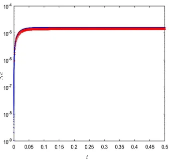
than the FD one. To achieve the same accuracy level of the IRBF time scheme, as shown in Figure
5, the FD time scheme needs a much smaller time step (i.e. ∆t = 10−6). The obtained results
of this example demonstrate that the proposed compact time stencil has the ability to work with
4.1.2 Two dimensional space
The PDE to be considered here is in the form of
∂f
∂t (x, y, t)−
∂2f
∂x2 (x, y, t) +
∂2f
∂y2 (x, y, t)
= 3etsin (x) sin (y), (41)
The exact solution is given by
fe(x, y, t) = sin(x) sin(y)et. (42)
This function grows exponentially with time and thus provides a good test for the proposed
compact time stencil. The initial values and Dirichlet boundary conditions can be derived from
(42).
We consider two types of domains, a unit square and a multiply-connected domain that is a region
lying between a unit square and a circle of radius 0.2. The explicit approach is employed to obtain
the numerical solutions of (41).
For the unit square, to examine accuracy of the proposed compact time stencils, we also implement
the forward differences. These two time approximation schemes are employed with the same time
step of 10−3 and the same spatial approximation that is based on central differences on a grid
density of 10×10. Figure 6 shows that a much improved accuracy is obtained with the proposed scheme (βt = 12). It is noted that the accuracy is computed over the whole spatial domain. As
also shown in the figure, a further improvement can be achieved by replacing the spatial central
differences with the compact 5-node IRBF stencils using βs = 3.5. For the multi-connected
domain, because of its non-rectangular shape, we only employ the compact 5-node IRBF stencils
for the spatial approximation. The obtained results on a grid density of 22×22 and with ∆t = 10−4
are more accurate than those by the forward differences.
4.2
Example 2: Convection-Diffusion equations
The proposed method is further verified with the convection-diffusion equations in one and two
dimensional space.
4.2.1 One dimensional space
Consider the following equation
∂f
∂t (x, t) +f(x, t) ∂f
∂x(x, t) = ∂2f
∂x2 (x, t) + 2 sin (x)e
t
+ sin (x) cos (x)e2t, (43)
on an interval [0,1] with the initial and boundary conditions
f(x,0) = sin (x), (44)
f(0, t) = 0, (45)
f(1, t) = sin (1)et. (46)
The exact solution to this problem can be verified to be fe(x, t) = sin(x)et.
We employ compact 3-point IRBF stencils on a grid of 10 nodes with βs = 3.5 for the spatial
approximation, and compact 2-point IRBF stencils for the temporal approximation. Attention
here is given to the effects of the RBF width in the time domain on the solution accuracy. The
obtained results at a time step of 10−3 are shown in Figure 8. Results by the forward differences
are also included for comparison purposes. It can be seen that better accuracy can be achieved
∆t; however, changingβt does not lead to any increase in computational cost.
4.2.2 Two dimensional space
An unsteady convection-diffusion equation in two dimensional space for a variable f can be
ex-pressed as
∂f
∂t (x, y, t) +cx ∂f
∂x(x, y, t) +cy ∂f
∂y (x, y, t) = dx ∂2f
∂x2 (x, y, t) +dy
∂2f
∂y2 (x, y, t) +b(x, y, t). (47)
Here, we choose cx =cy = 0.01, dx =dy = 1 and
b(x, y, t) = 3 sin (x) sin (y)r+ 0.01r(cos (x) sin (y) + cos (y) sin (x)).
The domain of interest is of [0,1]×[0,1] and the initial and boundary conditions are given by
u(x, y,0) = sin (x) sin (y), (48)
u(0, y, t) =u(x,0, t) = 0, (49)
u(1, y, t) = sin (1) sin (y)r, (50)
u(x,1, t) = sin (x) sin (1)r, (51)
where
r = 1 +t+t
2
2 +
t3
6 +
t4
24+
t5
120.
This problem has the following exact solution
fe(x, t) = sin(x) sin(y)r. (52)
The problem domain is represented by a Cartesian grid of 10×10. Other parameters employed are
the proposed compact time scheme outperforms the conventional forward differences. Similar
remarks to the case of one dimensional space can also be made here. In particular, the solution
accuracy can be enhanced by changing the MQ width (βt) without any additional computational
cost.
4.3
Example 3: Shallow water equations (SWEs)
RBF methods have been applied to solve the shallow water equations (SWEs). Their solutions are
reported using the global MQ approximation [18-20], compactly supported radial-basis function
(CSRBF) [21] and local radial-basis-function differential quadrature (LRBFDQ) [22] methods. In
these works, the time derivative term is approximated by conventional finite-difference schemes.
For SWEs, there are two dependent variables, namely the water height in thez direction, denoted
by h, and the velocity vector in the x−y plane, denoted by (u, v). They are functions of spacex
and time t.
The continuity and momentum SWEs can be linearised as follows
∂h
∂t (x, y, t) +H
∂u
∂x(x, y, t) + ∂v
∂y (x, y, t)
= 0, (53)
∂u
∂t (x, y, t) +g ∂h
∂x(x, y, t) = 0, (54) ∂v
∂t (x, y, t) +g ∂h
∂y(x, y, t) = 0, (55)
whereg = 9.81m/s2. For convenience, the water depthhcan be regarded as the sum of the mean
water depth H and the water surface elevation ζ.
Consider a rectangular channel of lengthL= 872km and widthW = 50km with the fluid being
The boundary condition for the water surface elevation is specified as
ζ(x, y, t) =ζ0cosat,
at x= 0, 0 ≤y ≤W, ζ0 = 1 m and a = 1.45444×10⁻⁴s−1, while the land boundary conditions
are
u(x, y, t) = 0,
atx=L, 0≤y≤W and
u(x, y, t) = 0,
aty= 0 and y=W, 0≤x≤L. The initial conditions are prescribed as
u(x, y, t= 0) = 0, (56)
v(x, y, t= 0) = 0, (57)
ζ(x, y, t= 0) =ζ0cos
a
√
gH (L−x)
/cos a √ gHL . (58)
This fluid flow problem has the following exact solution
ζ(x, y, t) = ζ0cos
a
√
gH(L−x)
cosat/cos
a √ gHL , (59)
u(x, y, t) =−ζ0
r g H sin a √
gH (L−x)
sinat/cos
a √ gHL , (60)
v(x, y, t) = 0. (61)
As in [22], for comparison purposes, we also discretise the fluid domain using a set of 205 collocation
[image:18.612.147.555.335.577.2]points and employ a time step of 30 s. The results obtained from proposed method are shown in
Table 1 together with those by the global-MQ method [20], CSRBF method [21] and LRBFDQ
method employed with 9 (R9) and 13 (R13) local nodes per approximation [22]. The temporal term
methods, and full-implicit FD scheme for LRBFDQ. All the numerical results displayed in Table 1
are computed att = 43200s and at three particular points 102, 103, and 104 which are located at
the center of the basin (Figure 10). The units of water depth and velocity used arecmand cm/s,
respectively. Errors for the water height and velocities are also measured by means of RMSE
and MAE defined in (36) and (37), respectively. It can be seen that the proposed method yields
the most accurate results. Figure 11 shows the water free surfaces at two time levels (t= 14400s
and t= 43200s) and the IRBF results look feasible when compared to the analytic solutions.
4.4
Example 4: Buoyancy-driven flows
In this example, natural convection between a heated inner circular cylinder of diameter Di and
a cooled square enclosure of side length D is considered (Figure 12). This problem has been
investigated with both experimental and numerical works. The latter was conducted by a variety
of numerical techniques such as the finite-difference methods [23,24], finite-element methods
[25-27], finite-volume methods [28,29], RBF-based methods [30], lattice Boltzmann methods [31,32]
and spectral methods [33-35]. The governing equations can be written in terms of the stream
function (ψ), vorticity (ω) and temperature (T)
∇2ψ =ω, (62)
∂ω
∂t + (u·∇)ω=
r
P r Ra∇
2ω
−∂T
∂x, (63)
∂T
∂t + (u·∇)T =
1
√
RaP r∇
2T, (64)
where u is the velocity vector (u = ∂ψ/∂y and v = −∂ψ/∂x), and P r and Ra the Prandtl and Rayleigh numbers defined as P r = ν/γ and Ra = βg∆T D3/γν, in which ν is the kinematic
We employ an aspect ratio of D/Di = 2.5, P r = 0.71 and Ra= {104,5×104,105,5×105,106}.
Non-slip boundary conditions and the symmetry of flow about the vertical centreline lead toψ = 0
and ∂ψ/∂n= 0 (n - the normal direction) on the inner and outer boundaries. Following [36], we
derive boundary conditions for equation (63). The values of the vorticity at the boundary nodes
on thex and y grid lines can be computed by
ωb = [1 + (
y x)
2]∂2ψb
∂x2 , (65)
ωb = [1 + (
x y)
2]∂2ψb
∂y2 , (66)
respectively. The boundary conditions for (64) are T = 1 and T = 0 on the inner and outer
surfaces, respectively.
The fluid domain is discretised using a grid density of 30×30. The three equations (62)-(64) must be solved simultaneously; an iterative scheme, where the convection terms are treated explicitly, is
employed to obtain a convergent solution with time. When the difference between two successive
stream function fields can be negligible, the flow is considered to reach the steady state. Numerical
experiments indicate that the proposed compact time stencil can work with larger time step than
the conventional finite difference scheme, leading to a faster convergence as shown in Figure 13.
The obtained velocity vector field and contour plots of the temperature are displayed in Figure
14, where 21 contour lines are used with their levels varying linearly between the minimum and
maximum values. They look feasible when compared to existing results by other methods.
One important result of this type of flow is the local heat transfer coefficient defined as [29]
Θ =−l∂T
∂n, (67)
gradient at the wall to a reference temperature gradient) is computed by
Nu= Θ
l , (68)
where Θ =−H ∂T
∂nds. Since the computational domain in [29] is taken as one-half of the physical
domain, values of Nu in the present work are divided by 2 for comparison purposes. Results
concerningNufor several values ofRaare shown in Table 2 along with those reported in [29,36,37].
It can be seen that they are in good agreement. Especially, for highly nonlinear solutions (e.g.
Ra= 106), the result obtained from the proposed method is very close to that of the differential
quadrature method [37] but without the need of doing coordinate transformation.
5
Concluding remarks
In this study, a new approximation scheme for the time derivative term is proposed. The time
stencil is based on 2 nodes over which integrated RBFs are employed to represent the field variable.
In addition, apart from two nodal values of the field variable, its derivative value at the first node
of the stencil is also included the approximation. When compared to conventional first-order
finite differences, numerical results indicate that larger time steps can be employed with the
proposed time discretisation scheme. In this work, we combine the proposed time scheme with
the space compact 5-point IRBF stencils, resulting in a numerical procedure, based on compact
IRBF approximations only, for solving parabolic PDEs. The method is applied to simulate shallow
water flows in large-scale domains and natural convection flows in multiply-connected domains,
and produces accurate results using relatively large time steps.
Acknowledgements
This research is supported by Computational Engineering andMechanics and Informatics (IAMI), HCMC Vietnam Academy of Science and Technology (VAST).
References
1. N. Mai-Duy, and T. Tran-Cong, A compact five-point stencil based on integrated RBFs for 2D second-order differential problems, Journal of Computational Physics, vol. 235, pp. 302-321, 2013.
2. G.E. Fasshauer,Meshfree Approximation Methods with Matlab, World Scientific, New Jersey, 2007.
3. W. Chen, Z.J. Fu, and C.S. Chen, Recent Advances in Radial Basis Function Collocation Methods, Springer, Berlin, 2014.
4. E.J. Kansa, Multiquadrics-A scattered data approximation scheme with applications to com-putational fluid-dynamics-II solutions to parabolic, hyperbolic and elliptic partial differential equations,Computers and Mathematics with Applications, vol. 19, no. 8, pp. 147-161, 1990.
5. N. Mai-Duy, and T. Tran-Cong, Numerical solution of differential equations using multi-quadric radial basis function networks, Neural Networks, vol. 14, pp. 185-199, 2001.
6. J. Waters, and D.W. Pepper, Global versus localized RBF meshless methods for solving incompressible fluid flow with heat transfer,Numerical Heat Transfer, Part B: Fundamentals, vol.68, no. 3, pp. 185-203, 2015.
7. Z.H. Wang, Z. Huang, W. Zhang, and G. Xi, A meshless local radial basis function method for two-dimensional incompressible Navier-Stokes equations,Numerical Heat Transfer, Part B: Fundamentals, vol. 67, no. 4, pp. 320-337, 2015.
8. E. Divo, and A.J. Kassab, An efficient localized radial basis function meshless method for fluid flow and conjugate heat transfer,Journal of Heat Transfer, vol. 129, no. 2, pp. 124-136, 2007.
9. N. Mai-Duy, and T. Tran-Cong, A Cartesian-grid discretisation scheme based on local inte-grated RBFNs for two-dimensional elliptic problems, CMES: Computer Modeling in Engi-neering and Sciences, vol. 51, no. 3, pp. 213-238, 2009.
10. N. Mai-Duy, and T. Tran-Cong, Compact local integrated-RBF approximations for second-order elliptic differential problems, Journal of Computational Physics, vol. 230, no. 12, pp. 4772-4794, 2011.
11. C. Shu, H. Ding, and K. Yeo, Local radial basis function-based differential quadrature method and its application to solve two-dimensional incompressible Navier-Stokes equa-tions, Computer Methods in Applied Mechanics and Engineering, vol. 192, no. 7-8, pp. 941-954, 2003.
13. N. Thai-Quang, K. Le-Cao, N. Mai-Duy, C.D. Tran, and T. Tran-Cong, A numerical scheme based on compact integrated-RBFs and AdamsBashforth/CrankNicolson algorithms for dif-fusion and unsteady fluid flow problems,Engineering Analysis with Boundary Elements, vol. 37, no. 12, pp. 1653-1667, 2013.
14. Y.L. Wu, and G.R. Liu, A meshfree formulation of local radial point interpolation method (LRPIM) for incompressible flow simulation, Computational Mechanics, vol. 30, no. 5-6, pp. 355-365, 2003.
15. C.M.T. Tien, N. Thai-Quang, N. Mai-Duy, C.D. Tran, and T. Tran-Cong, A three-point coupled compact integrated RBF scheme for second-order differential problems, CMES: Computer Modeling in Engineering and Sciences, vol. 104, no. 6, pp. 425-469, 2015.
16. G.B. Wright, and B. Fornberg, Scattered node compact finite difference-type formulas gen-erated from radial basis functions, Journal of Computational Physics, vol. 212, no. 1, pp. 99-123, 2006.
17. N. Mai-Duy, and T. Tran-Cong, A Cartesian-grid collocation method based on radial basis function networks for solving PDEs in irregular domains, Numerical Methods for Partial Differential Equations, vol. 23, no. 5, pp. 1192-1210, 2007.
18. Y.C. Hon, K.F. Cheung, X.Z. Mao, and E.J. Kansa, Multiquadric solution for shallow water equations, Journal of Hydraulic Engineering, vol. 125, no. 5, pp. 524-533, 1999.
19. D.L. Young, S.C. Jane, C.Y. Lin, C.L. Chiu, and K.C. Chen, Solutions of 2D and 3D Stokes laws using multiquadrics method, Engineering Analysis with Boundary Elements, vol. 28, no. 10, pp. 1233-1243, 2004.
20. D.L. Young, C.S. Chen, and T.K. Wong, Solution of Maxwell’s equations using the MQ method,Computers, Materials & Continua, vol. 2, pp. 267-76, 2005.
21. S.M. Wong, Y.C. Hon, and M.A. Golberg, Compactly supported radial basis functions for shallow water equations,Applied Mathematics and Computation, vol. 127, no. 1, pp. 79-101, 2002.
22. C.P. Sun, D.L. Young, L.H. Shen, T.F. Chen, and C.C. Hsian, Application of localized mesh-less methods to 2D shallow water equation problems, Engineering Analysis with Boundary Elements, vol. 37, no. 11, pp. 1339-1350, 2013.
23. G. De Vahl Davis, Natural convection of air in a square cavity: a bench mark numerical solution, International Journal for Numerical Methods in Fluids, vol. 3, no. 3, pp. 249-264, 1983.
24. T.H. Kuehn, and R.J. Goldstein, An experimental and theoretical study of natural convec-tion in the annulus between horizontal concentric cylinders,Journal of Fluid Mechanics, vol. 74, no. 4, pp. 695-719, 1976.
25. M.T. Manzari, An explicit finite element algorithm for convection heat transfer problems,
26. H. Sammouda, A. Belghith, and C. Surry, Finite element simulation of transient natural convection of low-Prandtl-number fluids in heated cavity,International Journal of Numerical Methods for Heat and Fluid Flow, vol. 9, no. 5, pp. 612-624, 1999.
27. L. Jin, and H. Shen, Projection-and characteristic-based operator-splitting simulation of mixed convection flow coupling heat transfer and fluid flow in a lid-driven square cavity,
Numerical Heat Transfer, Part B: Fundamentals, vol. 70, no. 4, pp. 354-371, 2016.
28. E.K. Glakpe, C.B. Watkins Jr, and J.N. Cannon, Constant heat flux solutions for natural convection between concentric and eccentric horizontal cylinders, Numerical Heat Transfer, Part A: Applications, vol. 10, no. 3, pp. 279-295, 1986.
29. F. Moukalled, and S. Acharya, Natural convection in the annulus between concentric hori-zontal circular and square cylinders, Journal of Thermophysics and Heat Transfer, vol. 10, no. 3, pp. 524-531, 1996.
30. B. Sarler, J. Perko, and C.S. Chen, Radial basis function collocation method solution of natural convection in porous media, International Journal of Numerical Methods for Heat and Fluid Flow, vol. 14, no. 2, pp. 187-212, 2004.
31. Y. Wang, C. Shu, C. J. Teo, and L. M. Yang, A fractional-step lattice Boltzmann flux solver for axisymmetric thermal flows, Numerical Heat Transfer, Part B: Fundamentals, vol. 69, no. 2, pp. 111-129, 2016.
32. A. J. Ahrar, and M. H. Djavareshkian, Novel hybrid lattice Boltzmann technique with TVD characteristics for simulation of heat transfer and entropy generations of MHD and natural convection in a cavity, Numerical Heat Transfer, Part B: Fundamentals, vol. 72, no. 6, pp. 431-449, 2017.
33. P. Le Quere, Accurate solutions to the square thermally driven cavity at high Rayleigh number,Computers and Fluids, vol. 20, no. 1, pp. 29-41, 1991.
34. C. Shu, Application of differential quadrature method to simulate natural convection in a concentric annulus, International Journal for Numerical Methods in Fluids, vol. 30, no. 8, pp. 977-993, 1999.
35. Z. Wang, Z. Huang, W. Zhang and G. Xi, A multidomain chebyshev pseudo-spectral method for fluid flow and heat transfer from square cylinders, Numerical Heat Transfer, Part B: Fundamentals, vol. 68, no. 3, pp. 224-238, 2015.
36. K. Le-Cao, N. Mai-Duy, and T. Tran-Cong, An effective integrated-RBFN Cartesian-grid discretization for the stream function vorticity temperature formulation in nonrectangular domains, Numerical Heat Transfer, Part B: Fundamentals, vol. 55, no. 6, pp. 480-502, 2009.
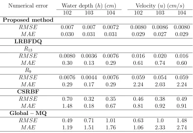
Table 1: Example 3, shallow water flows: Comparison of numerical errors at three nodes 102, 103, and 104 between the proposed method and the LRBFDQ, CSRBF and global MQ methods.
Numerical error Water depth (h) (cm) Velocity (u) (cm/s) 102 103 104 102 103 104
Proposed method
RMSE 0.007 0.007 0.0072 0.0080 0.0086 0.0080
MAE 0.030 0.031 0.031 0.029 0.027 0.029
LRBFDQ
R13
RMSE 0.0080 0.0036 0.0076 0.016 0.020 0.016
MAE 0.30 0.13 0.29 0.61 0.74 0.60
R9
RMSE 0.0076 0.0044 0.0076 0.059 0.054 0.059
MAE 0.29 0.17 0.29 2.24 2.03 2.24
CSRBF
RMSE 0.70 0.32 0.35 0.46 0.38 0.49
MAE 1.48 0.18 0.67 0.81 0.92 0.91
Global−MQ
RMSE 0.49 0.71 1.01 0.63 1.0 1.48
Table 2: Example 4, natural convection: Comparison of the average Nusselt number between the proposed method and some other methods for Ra in the range of 104 to 106.
Ra 104 5×10⁴ 105 5×10⁵ 106
Nu
Proposed method 3.23 4.04 4.88 7.68 9.38 1D IRBF [36] 3.22 4.04 4.89 7.43 8.70
FVM [29] 3.24 4.86 8.90
1 3 5
2 4
∂
Ω
[image:27.612.108.506.48.298.2]Ω
t
f
∂f ∂t
k−1
f
k−1f
k
[image:28.612.118.501.53.363.2]t
k−1t
kt
f
(
x
,t
[image:29.612.137.471.53.367.2])
t
N
[image:30.612.140.464.49.368.2]e
Figure 4: Example 1.1, parabolic PDE, spatial compact IRBF stencils, ∆t = 10−3: Comparison
t
N
[image:31.612.139.476.50.369.2]e
Figure 5: Example 1.1, parabolic PDE, spatial compact IRBF stencils: Comparison of the solution accuracy between the FD (‘·’, ∆t = 10−6) and the IRBF (‘×’, ∆t = 10−3, β
t = 18) time
t
N
[image:32.612.138.476.51.371.2]e
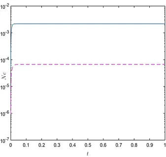
Figure 6: Example 1.2, parabolic PDE, rectangular domain, ∆t= 10−3: Numerical errors obtained
t
N
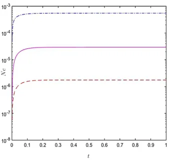
[image:33.612.137.474.51.370.2]e
Figure 7: Example 1.2, parabolic PDE, non-rectangular domain, spatial compact IRBF stencils, ∆t = 10−4 and β
t = 10: Numerical errors obtained by the FD time (‘−’) and IRBF time (‘- -’)
0 0.1 0.2 0.3 0.4 0.5 0.6 0.7 0.8 0.9 1 10-8
10-7 10-6 10-5 10-4
FD time IRBF time (t=10) IRBF time (t=12) IRBF time (t=15) IRBF time (t=17)
t
N
[image:34.612.154.458.69.353.2]e
Figure 8: Example 2.1, 1D convection-diffusion equation, ∆t = 10−3: Effect of the temporal RBF
width, represented through βt (βt= 10, 12, 15, 17), on the IRBF solution accuracy. Results by
0 0.1 0.2 0.3 0.4 0.5 0.6 0.7 0.8 0.9 1 10-8
10-7 10-6 10-5 10-4 10-3
FD time IRBF time (
t=3)
IRBF time (
t=7)
IRBF time (
t=10)
IRBF time (
t=12)
t
N
[image:35.612.132.480.70.407.2]e
Figure 9: Example 2.2, 2D convection-diffusion equation, ∆t = 10−3: Effect of the temporal RBF
width, represented through βt (βt= 3, 7, 10, 12), on the IRBF solution accuracy. Results by the
Number of iterations
C
on
ve
rg
en
ce
m
ea
su
[image:39.612.138.470.59.367.2]re
Figure 13: Example 4, natural convection, spatial compact IRBF stencils, ∆t = 0.02 (IRBF) and ∆t = 0.014 (FD), Ra = 105: The IRBF approximation with respect to time can work with a
Ra= 104
Ra= 105
[image:40.612.227.394.76.432.2]Ra= 106
![Table 1 together with those by the global-MQ method [20], CSRBF method [21] and LRBFDQ](https://thumb-us.123doks.com/thumbv2/123dok_us/144563.21707/18.612.147.555.335.577/table-global-mq-method-csrbf-method-lrbfdq.webp)