Increased classification rates of chemical detectors using novel sensor types and optimized sensing geometries

Novel Sensor Types and Optimized Sensing Geometries

Thesis by

Marc D. Woodka

In Partial Fulfillment of the Requirements

For the Degree of

Doctor of Philosophy

California Institute of Technology

Pasadena, California

2009

Acknowledgements

There are a number of people to whom I owe much thanks, many of whom I would not be here without. In chronological order: to start, I thank my parents for their love and support throughout the years. This is a thing often taken for granted, but it puts those who grew up with it at a tremendous advantage in life. Without this, I certainly would not be here today.

I also thank Prof. Georges Belfort and my graduate student mentor Dr. Gautam Baruah, who welcomed me as an undergraduate student researcher at Rensselaer Polytechnic Institute. They demonstrated to me an excitement and enthusiasm for research, and made my decision to attend graduate school at Caltech an easy one.

Thanks to my research advisor, Professor Nate Lewis, who allowed me the time and freedom to guide my research and overcome the hurdles at various steps throughout my graduate career – the extra time required to study for the qualifying exams, to learn various programming languages, to figure things out, etc. Also, thanks for your well-timed motivation and ideas, and finally, thanks for letting me represent the nose project at various points throughout the past few years – it mixed things up for me, and provided me with a greater appreciation for the grand scheme of things.

Many thanks are due to Dr. Bruce Brunschwig, effectively my second research advisor. During my first year, when I realized I needed to learn to program in LabVIEW, I looked to Bruce for assistance, and he immediately gave me several hours of his time and guidance. This was when I first recognized Bruce as an invaluable resource, and I have utilized him since for a number of meaningful discussions, from which I have learned much. He was also a very critical reviewer of all chapters in this thesis, which made the chapters come out better in the end. Thanks for the discussions, ideas, insights, and careful readings!

When I first joined the Lewis group, Brian Sisk and Ting Gao were the graduate student and post-doc, respectively, on the nose project. Thanks to Brian for introducing me to the lab and mentoring me in Matlab, and thanks to Ting for leaving behind some unfinished work, which became my first publication and formed Chapter 2 of my thesis. Also, when my research was just beginning, Mike Burl from JPL suggested using non-negative least squares for mixture analysis, which has since been the best performing algorithm for the task. I hopefully would have stumbled across it on my own, but we’ll never know… Thanks for the discussion and suggestion!

understand what was going on in my world of research, and offering suggestions and comments; Edgardo Garcia, for several collaborations and discussions, and for coming back from Puerto Rico; Stephen Maldonado, for collaborations and useful discussions; and Anna Folinsky and Heather McCaig, for interactions and discussions throughout the years. Also, thanks to everybody else from the Lewis group who has made my time here enjoyable and entertaining: Pat for getting me into diving; Craig for the visits and discussions; Cinco (Davy) for the trips to Grandma’s up at Big Bear and good conversation; Pat, Steve, Tony, Don, Craig and Edgardo for the fun outside of lab. Everybody else in the Lewis group not listed here: thanks for making the Lewis group a great place to spend 5 years.

Thanks to the Chemical Engineering support group: Shane for the many well-researched adventures; Armin for the laid-back attitude and the good times (Tucson was a blast); Andrew for the well-researched culinary options in the area (Hometown Buffet); and Ubaldo and Win for the good company at these culinary options. Also, thanks to Ameri for his time and patience during our first year, when he took the time to share with me his deep understanding of all things ChemE.

Thanks to my committee, Professors Rick Flagan, Mark Davis, and Pietro Perona, for their interest in my research project and for taking the time out of their schedule to read my thesis and sit on my committee. Special thanks to Rick Flagan for suggesting FEMLAB to solve my modeling issues during my candidacy – it took me over a year of fighting with an implicit finite-difference Crank-Nicholson scheme before I finally gave in, but when I did FEMLAB worked wonderfully.

Abstract

Broadly responsive vapor sensor arrays, or so-called “electronic noses,” have been explored and/or used for many years as a means to detect the vapors present in the headspace of a variety of targets, such as coffees, wines, vinegars, oils, explosives, and nerve agents, and for disease diagnosis. Electronic nose sensing modalities often exhibit a response that is linear with concentration, and additive with respect to multiple vapors. Ideally, one could simply train an array towards the pure vapors of interest, and use that pure vapor training to identify either pure vapors or vapor mixtures during field-testing. This, however, has proven difficult, and has limited the utility of this vapor detection approach for a number of applications.

This thesis utilized a low-cost, low-power sensing modality, insulator – carbon black composite chemiresistors, and exploited their linear response properties to enhance the classification rates of both pure vapors and vapor mixtures, based on pure vapor training. Sensors utilizing non-polymeric, small organic molecules as the insulating component were demonstrated to offer enhanced separation between pure vapor response clusters, and lower detection limits, relative to the traditional use of polymers as the insulating phase. These sensors were then used in a sensing geometry that induced a space- and time, or spatiotemporal (ST) dependence, to the sensor response, which increased the amount of chemical information extracted from the sensor response. This ST response information allowed for the correct classification of vapor mixtures consisting of up to 5 components, with training on only pure vapors.

A mass uptake model for the ST response of the sensors was developed, and vapor detection and mixture analysis was simulated for chamber geometries and vapor delivery flow rates spanning several orders of magnitude. The data were first used to define an optimized ST sensing regime for mixture analysis, based on two dimensionless Peclet number analogs. The data were then used to identify the inherent properties of the pure vapor training data that allowed for mixture analysis to be performed at high levels, specifically that the minimum resolution factor between all binary vapor combinations in the training library was sufficiently high.

Contents

Acknowledgements iii

Abstract v

List of Figures ix

List of Tables xii

1 Introduction: Electronic Noses and Polymer-Carbon Black

Composite Vapor Sensors 1

1.1 Electronic Nose Introduction . . . 1

1.2 Vapor Sensing with Insulator – Conductor Composites . . . 2

1.3 Outline of This Thesis . . . 5

1.4 References. . . 6

2 Chemiresistors for Array-Based Vapor Sensing Using Composites of Carbon Black with Low Volatility Organic Molecules 13 2.1 Abstract . . . 13

2.2 Introduction . . . 13

2.3 Experimental . . . 15

2.4 Results . . . 18

2.5 Discussion . . . 24

2.6 Conclusions . . . 25

2.7 References . . . 26

3 Use of Spatiotemopral Response Information from Sorption-Based Sensor Arrays to Identify and Quantify the Composition of Analyte Mixtures 42

3.1 Abstract . . . 42

3.2 Introduction . . . 43

3.3 Experimental . . . 45

3.4 Results . . . 50

3.6 Conclusions . . . 58

3.7 References . . . 59

4 Modeling of Spatiotemporal Response and the Definition of an Optimal Regime for Mixture Analysis 77

4.1 Abstract . . . 77

4.2 Introduction . . . 78

4.3 Experimental . . . 81

4.4 Results . . . 85

4.5 Modeling Formulation . . . 86

4.6 Modeling Results . . . 89

4.7 Discussion . . . 92

4.8 Conclusions . . . 95

4.9 Appendix . . . 96

4.10 References . . . 103

5 Evaluation of Pattern Recognition Techniques for Analysis of Vapor Mixtures Using Spatiotemporal Response 119

5.1 Abstract . . . 119

5.2 Introduction . . . 119

5.3 Experimental . . . 122

5.4 Results . . . 129

5.5 Discussion . . . 131

5.6 Conclusions . . . 135

5.7 References . . . 135

6 Enhancement of Pure Vapor Classification Rates Using Spatiotemporal Response 148 6.1 Abstract . . . 148

6.2 Introduction . . . 149

6.3 Experimental . . . 150

6.4 Results . . . 157

6.5 Discussion . . . 160

6.6 Conclusions . . . 163

7 Thesis Summary 177

List of Figures

1.1 Generic electronic nose architecture . . . 8 1.2 Resistance vs. volume fraction of conducting material demonstrating percolation

theory and its implications for insulator-conductor chemiresistive vapor sensors . . 9 1.3 Schematic representation of the smelling by swelling response mechanism . . . 10 1.4 Demonstration of the response linearity of polymer – carbon black composite

chemiresistive vapor sensors . . . 11 1.5 Demonstration of the response additivity of polymer – carbon black composite

chemiresistive vapor sensors . . . 12 2.1 Chemical structures of materials used to fabricate non-polymer – carbon black

composite vapor sensors . . . 36 2.2 Responses of non-polymer – carbon black and polymer – carbon black composite

Chemiresistive vapor sensors . . . 37 2.3 Response linearity of non-polymer – carbon black composite chemiresistive

vapor sensors on exposure to a) n-hexane and b) ethanol . . . 38 2.4 Three-dimensional representation of non-polymer – carbon black composite

sensor responses on exposure to various test analyte vapors . . . 39 2.5 Principal components analysis showing the natural clustering ability of a 7-array

non-polymer – carbon black composite (75% carbon black) on exposure to various test analytes . . . 40 2.6 Waterfall plots detailing the 6-month drift in FLD D-values for

n-hexane – isooctane classification with a) no calibration and b) calibration . . . 41 3.1 Schematic of the sensor substrates used to generate the spatiotemporal sensor

response . . . 68 3.2 Schematic of the chamber design used to generate the spatiotemporal sensor

response . . . 69

3.3 Spatiotemporal response of a 15-sensor array of propyl gallate/carbon black

(75% carbon black) to a) pure hexane and b) pure decane at P/Po _{= 0.050 . . . 70} 3.4 Spatiotemporal response of sensors 1 and 9 along a 15-sensor array to pure ethyl

acetate, pure decane, and a mixture of ethyl acetate and decane . . . 71 3.5 Comparison between various vapor sensing and pattern recognition methods for

3.6 Comparison between various vapor sensing and pattern recognition methods for the analysis of a 3-component vapor mixture . . . 73

3.7 Comparison between various vapor sensing and pattern recognition methods for the analysis of a 4-component vapor mixture . . . 74

3.8 Comparison between various vapor sensing and pattern recognition methods for the analysis of a 5-component vapor mixture . . . 75

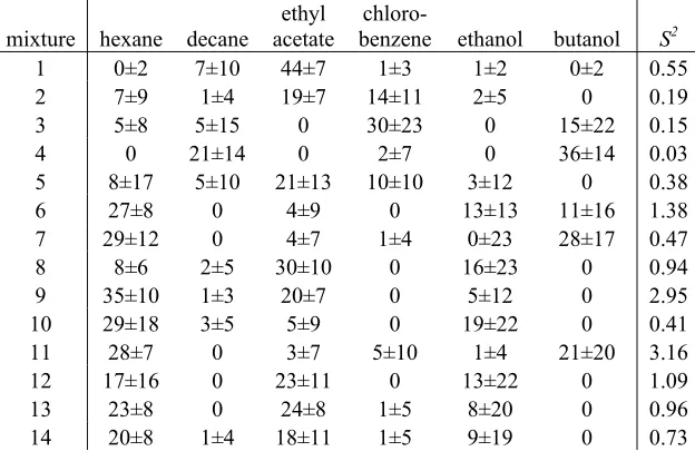
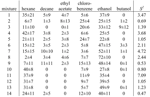
3.9 Residual squared error vs. mixture number for the fourteen vapor mixtures

Attempted, using various vapor sensing and pattern recognition approaches . . . 76 4.A1 To-scale representation of a hypothetical, unscaled chamber. . . 100 4.A2 To-scale representation of a scaled chamber . . . 101 4.1 Schematic of the arrangement used to optically monitor the vapor delivery to the

sensor chamber . . . 111 4.2 Shifts in a) sensor response and b) QCM frequency as a function of concentration

for various analyte vapors on exposure to a tetracosanoic acid – carbon black

composite vapor sensor . . . 112

4.3 The a) raw photodiode voltage response, b) baseline-corrected voltage response, and c) absorbance response profile of acetone vapor to the sensor chamber . . . 113

4.4 Depiction of the main equations used to model the mass uptake of the sensor

films . . . 114

4.5 Experimental and modeled responses for a 2.6 μm thick propyl gallate –

carbon black composite 15-sensor array exposed to hexane . . . 115 4.6 Experimental and modeled responses for a 2.6 μm thick propyl gallate –

carbon black composite 15-sensor array exposed to decane . . . 116 4.7 Experimental and modeled responses for a 1.5 μm thick tetracosane/dioctyl

phthalate – carbon black composite 15-sensor array exposed to a) pure ethyl

acetate, b) pure decane, and c) a mixture of ethyl acetate and decane . . . 117 4.8 Mixture analysis residual error (S2_{) vs. Peyz with varying Pezz cutoff values for}

modeled 0.1 μm films . . . 118 4.9 Mixture analysis residual error (S2_{) vs. Peyz with varying Pezz cutoff values for}

modeled 1.0 μm films . . . 119

5.1 Mixture analysis residual error (S2_{) vs. the number of principal components using} the a) variance (60%), b) variance (80%), c) eigenvalue ( ≥ 1), and

d) eigenvalue ( ≥ 2) methods; and e) the minimum resolution factor in the pure

the variance (80%) method for a) 5-, b) 7-, and c) 9-analyte training libraries . . . . 142

5.3 Mixture analysis residual error (S2_{) vs. number of principal components using the} eigenvalue ( ≥ 2) method for a) 5-, b) 7-, and c) 9-analyte training libraries . . . 143 5.4 Mixture analysis residual error (S2_{) vs. the minimum rf in the training library,}

from all binary pure vapor combinations, for a) 5-, b) 7-, and c) 9-analyte training libraries . . . 144 5.5 Mixture analysis residual error (S2_{) vs. number of principal components using the}

a) variance (80%) and b) eigenvalue ( ≥ 2) methods; and c) the minimum rf in the pure vapor training library, for various levels of superimposed Gaussian noise . . . 145

5.6 Analysis of a simulated 3-component mixture analyzed using a) NNLSQ,

b) EDPCR-limited, c) EDPCR-full, and d) PCR-SF . . . 146

5.7 Analysis of a simulated 4-component mixture analyzed using a) NNLSQ,

b) EDPCR-limited, c) EDPCR-full, and d) PCR-SF . . . 147

5.8 Mixture analysis residual error (S2_{) vs. the minimum rf in the vapor library, with} mixtures analyzed using NNLSQ, EDPCR-full, and PCR-SF . . . 148 6.1 ST array response of tetracosane/dioctyl phthalate – carbon black composite on

exposure to hexane, heptane, octane, nonane, and decane . . . 173 6.2 Waterfall plots detailing discrimination amongst the different vapor classes at

various steps of the FLD-HC classification algorithm . . . 174,175

List of Tables

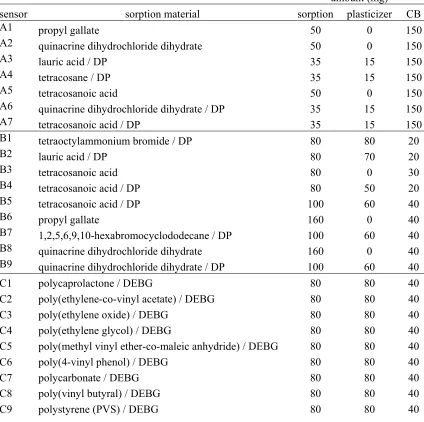
2.1 Materials used for the fabrication of non polymer – carbon black composite sensors using (A1-A7) 75% and (B1-B) 20% carbon black, and (C1-C9)

polymer-carbon black composite sensors using 20% carbon black . . . 28

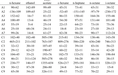
2.2 Sensor response (μ 10,000) of sensors A1-A7 and C1-C9 on exposure to various test analytes delivered at P/Po _{= 0.050}

. . . 29

2.3 Signal to noise ratios of sensors A1-A7 and C1-C9 on exposure to various test analytes delivered at P/Po _{= 0.050}

. . . 30

2.4 Limits of detection of sensors A1-A7, C1-C3, and C8 on exposure to n-hexane and ethanol . . . 31

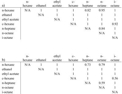
2.5 Testing resolution factors for binary analyte classification tasks using an array of a) sensors A1-A7 and b) sensors C1-C9 . . . 32

2.6 Binary classification rates of an array of sensors B1-B9 a) immediately following training, and b) two days, c) six days, and d) six months after training . . . 33,34

2.7 Classification rates of an array of sensors B1-B9 six months after the initial

training protocol, using different test analytes for calibration . . . 35

3.1 Sensor suspensions used to spray the linear non-polymer – carbon black

chemiresistive ST sensor arrays . . . 62

3.2 Fractional vapor pressures (μ 1000) of analyte vapors present in each of the 14 vapor mixtures, as determined by GC-MS . . . 63 3.3 Fractional vapor pressures (μ 1000) of analyte vapors present in each of the 14

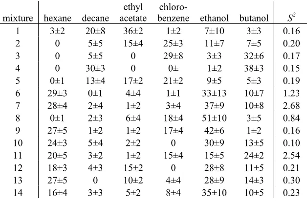
vapor mixtures, as determined by NNLSQ using ST analysis and all 15 sensors along each array . . . 64

3.4 Fractional vapor pressures (μ 1000) of analyte vapors present in each of the 14 vapor mixtures, as determined by EDPCR using ST analysis and all 15 sensors along each array . . . 65

3.5 Fractional vapor pressures (μ 1000) of analyte vapors present in each of the 14 vapor mixtures, as determined by NNLSQ using ST analysis and the first, middle, and last sensor along each array . . . 66 3.6 Fractional vapor pressures (μ 1000) of analyte vapors present in each of the 14

vapor mixtures, as determined by NNLSQ using SS analysis and the first three

4.1 Non-polymer – carbon black composite sensors used in this study . . . 105

4.2 Analyte abbreviations used in this work . . . 106

4.3 Calculated partition coefficients and sensor response slopes for all sensor – vapor combinations . . . 107

4.4 Geometries and flow rates used for macro-dimensioned modeling . . . 108

4.5 Geometries and flow rates used for micro-dimensioned modeling . . . 109

4.6 Fractional vapor pressures (μ 100) of modeled mixtures . . . 110

5.1 Non-polymer – carbon black composite sensors used in this study . . . 139

5.2 Analyte abbreviations used in this work . . . 140

6.1 Non-polymer – carbon black composite sensors used in this study . . . 167

6.2 Analyte abbreviations used in this work . . . 168

6.3 Testing resolution factors for all binary vapor combinations using the ST and SS detection approaches . . . 169

6.4 Testing confusion matrix for vapor classification using the kNN method and the ST and SS detection approaches . . . 170

6.5 Testing confusion matrix for vapor classification using the FLD-HC method and the ST and SS detection approaches . . . 171

Chapter 1

Introduction: Electronic Noses and

Polymer-Carbon Black Composite Vapor Sensors

1.1.

Electronic Nose Introduction

No man-made sensor system combines the sensitivity, low power, rapid response, selectivity, and ability to track an odorant to its source that is characteristic of the olfactory system of a canine. In mammals, G-protein-coupled receptors (GPCRs) are a broad class of trans-membrane receptors that are used in many physiological processes, such as visual transduction, hormonal regulation, and stimulation and inhibition of various processes.1 _{The mammalian genome possess}

at least 1,000 olfactory receptor genes2 _{that are part of the broader GPCRs class. Hence,}

olfactory receptors constitute the largest family of GPCRs in mammals. These º1,000 genes can potentially encode up to º1,000 different functional odor receptors. However, mammals are able to detect over 10,000 different odors. Thus, the receptors must be broadly responsive in their response properties. In this architecture, a given receptor will be triggered by more than one odorant, and an odorant, in turn, will produce a response from more than one receptor.3 _Olfactory

receptors are triggered in the olfactory epithelium, and then send a response through the olfactory bulb to the brain, for processing and odorant identification.

This biological process of olfaction lays the foundation for artificially created “electronic noses.” Electronic noses began to develop into their modern form in the mid-1980s. Prior to this, broadly responsive sensor arrays had been investigated to a limited extent; however, bottlenecks in electronics and computational capability limited progress.4,5 _{New technologies have been}

developed, and implementations of various pattern recognition algorithms, the workhorse of any electronic nose configuration, have flourished in the past 15 years.

exposed to the sensor array, generating a time-varying sensor signal, Si,j(t). Each of these sensor

signals is then processed, and a single metric response descriptor is generated for each sensor, creating an array response. During a training phase, the array is exposed numerous times to odorants that will be used later to challenge the array in identification tasks. The training process creates an odorant database. During subsequent testing of unidentified odorants, the array response is compared against the training library, and a prediction is made as to the identity and concentration of the odorant. Various levels of processing are required, and ultimately some form of pattern recognition is used to identify the odorant, mimicking the steps involved in odor identification in the mammalian olfactory system.

Electronic noses implement this generic architecture in various ways. Surface acoustic wave devices,6,7 _{tin oxide sensors,}8,9 _{conducting organic polymers,}10,11 _{polymer-coated quartz crystal}

microbalances,12,13 _{polymer-coated micromachined cantilevers,}14 _{dye-impregnated polymers}

coated onto optical fibers or beads,15,16 _{and polymer composite chemically sensitive resistors}17,18

comprise only a few of the broadly responsive sensors that have been employed in the construction of electronic noses. Pattern recognition algorithms that have been used include linear, statistically based methods such as partial least squares, principal components analysis (PCA), Fisher’s linear discriminant (FLD), k-nearest neighbors, and soft independent modeling of class analogy; as well as non-linear, non-statistical methods that include various implementations of artificial neural networks.8,19-21 _{This thesis will detail the recent developments of one sensing}

modality that has been developed at Caltech: insulator-carbon back composite chemiresistors.

1.2.

Vapor Sensing With Insulator – Conductor Composites

1.2.1.

Phase Equilibrium

When two phases come into contact, equilibrium will eventually be established for all species present. This is true regardless of the types of phases involved. The equilibration process between a vapor and a solid sorption based material forms the basis of sorption-based sensors.

Consider a vapor in equilibrium with an ideal solution of the vapor in a solid sorbent. In ideal solutions at equilibrium, Raoult’s law is followed for all components.22,23 _Thus:

o A s

A x P

P =

,

o A A s

P

P

x

=

.

The mole fraction, and consequently, the molarity, molality or weight percent of the vapor in the solid is a function of the ratio of the pressure exerted on the solid by species A divided by the vapor pressure of pure A. Therefore, for an ideal solution, the solubility of a vapor in any sensor material is a function only of the properties of the vapor, and not the solid.

For non-ideal solutions, eq (1) can be written in terms of activities:22,23

o A s A o A s A

A

a

P

x

P

P

=

=

γ

,

where aA,s is the activity of vapor species A in the solid, γA is the activity coefficient of species A in the solid, and the vapor is assumed to be an ideal gas at ambient pressure. For real solutions, Henry’s law is a better approximation for the solute then Raoult’s law, hence:

s H

A

k

x

P

≈

,

where kH is the Henry’s law constant, equal to γA

P

H A o A A A s

k

P

P

P

x

=

=

γ

1

.

The interactions between the solid and vapor that are responsible for the differences in solubilities of a given gas in different solids, and the differences in Henry’s law constants, or more generally the non-ideality, are therefore taken into account by differences in the activity coefficient for each gas/solid combination. The equilibrium mole fraction of the species in the solid is therefore dictated by the ratio of the pressure exerted by the species on the solid to the vapor pressure of the species, divided by the activity coefficient (eq (5)).

1.2.2. Insulator – Conductor Systems and Percolation Theory

loading of the conductor, and small increases in the loading of the conductor will then produce large increases in the conductivity of the composite.

Quantitatively, the resistance, R, of an insulator-conductor composite can be expressed as:

2 / 1 2 2 1 2

1 [( ) 2( 2) ]

) 2 ( m c m c R R z B B B B R R z R − + + + + −

=

,

where

B

=

R

[

−

1

+

(

z

/

2

)(

1

−

υ

/

f

)]

and

]

1

))

2

/(

[(

2

=

R

z

f

−

B

υ

.

Here, Rc and Rmare the resistances of the pure conducting and insulating substances, respectively;

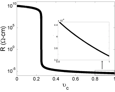
z is the coordination number for the conducting particles in the insulating matrix (which takes into account how the two substances pack); υc is the volume fraction of conducting material in the composite; and f is the total packing fraction of the composite (f ≤1).24,25 _{Figure 1.2 plots R}

vs. υc for a hypothetical insulator-conductor composite with Rc = 10-5 Ω-cm, Rm = 1010Ω-cm, z =

4, and a total packing fraction of f = 0.5. The percolation threshold, υp, is denoted by the sharp

drop in the resistance at a conducting volume fraction υc= υp= 0.25, i.e., the volume fraction of conducting material at the percolation threshold υp = 2f/z.

1.2.3. Sensing Due to Phase Equilibration Using Percolative

Chemiresistor Sensors

When an insulator-conductor composite is exposed to various vapor environments, the composite will come to equilibrium with each species (odorant) in the vapor phase. Assuming that the analyte diffuses throughout the composite, its volume will increase to accommodate the presence of the analyte (Figure 1.3). This increase in volume will decrease υc. Assuming that the sorbed

material is non-conducting, the resistance of the composite will therefore increase.

Various materials have been used for the insulating and conducting phases of such sensors. The insulating phase is typically a low glass-transition temperature polymer or polymer blend, and the conducting phase is typically carbon black.18,24 _{However, insulating phases have included}

ligands chemically attached to conductive gold nanoparticle cores,26 _{and the conductive phase has}

included gold nanoparticles,26 _{conductive polymeric materials,}17,27,28 _{and could include other}

materials such as colloidal Ag, colloidal Au, or colloidal TiO2.

1.2.4. Polymer-Carbon

Black

Composite Chemiresistor Properties:

Response Linearity and Additivity

The ability to adjust the relative amount of the conducting material in the insulator – conductor composites allow choice of the regime in which the sensor will operate: close to the percolation threshold, or in the linear regime having a high concentration of the conductive component. Operation in the linear regime, while less sensitive, is generally preferred. In this regime, the response is directly proportional to the concentration of analyte vapor. This relationship results in a linear correlation between the sensor response and the concentration of individual components of the vapor mixtures. This linear relationship can, of course, break down at high odorant concentrations.

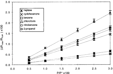
Figure 1.4 shows the equilibrium sensor response for a poly(butadiene)-carbon black composite vapor sensor (20% mass fraction of carbon black) upon exposure to various odorants at different fractions of their vapor pressures.29 The sensor exhibits a linear response with increasing concentration, until either the percolation threshold is reached for the sensor (not normally possible for high carbon black loadings) or until the sorption isotherm becomes nonlinear with vapor concentration.4

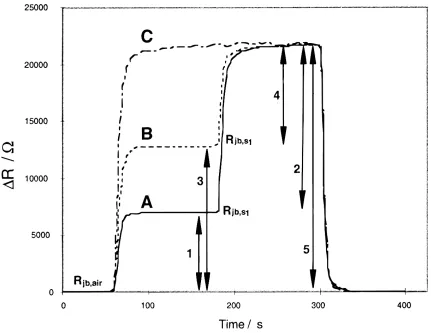
In the linear response regime, the sensor response to a mixture of odorants is simply the sum of the individual responses to the odorants that comprise the mixture. For example, Figure 1.5 displays the response of a prototypical sensor upon exposure to some test mixtures of odorants. In this experiment, benzene and chloroform were each exposed to the sensor at 2% of each of their vapor pressures (4600 ppm for chloroform and 2200 ppm for benzene) separately, and then in combination.29 For each odorant at the given concentration, the sensor exhibited a characteristic increase in resistance, regardless of the other odorants present. The sensor response was both additive and independent of the order of exposure.

1.3.

Outline of This Thesis

1.4 and 1.5, respectively, regardless of whether the unknown vapors are present in the pure form or as vapor mixtures, the array will only require training on the pure vapor components. This work addresses this task using a number of different approaches. Non-polymeric – carbon black composite chemiresistor sensors are introduced and demonstrated as a promising alternative to the traditional polymer – carbon black composite approach, wherein a higher concentration of functional groups present in the sorptive component of the sensor composite allows for enhanced vapor – sensor interactions, and an enhanced ability to discriminate between chemically similar vapors (Chapter 2) This work was started by a post-doc in our laboratory and left unfinished – my contribution was everything except the initial fabrication and analysis of the non polymer – carbon black composites (20% CB): this included the development of all figures, tables, analyses and discussions presented. Further, a means of increasing the amount of information extracted from sensor arrays is demonstrated by invoking a space- and time-, or spatiotemporal (ST) dependency, of the array’s response. This ST approach takes advantage of the linear and additive response properties of the sensors, and is demonstrated to significantly improve the ability of the sensors to identify and quantify vapor mixtures with training on only the pure vapor components (Chapter 3). A model for the ST response of sensor arrays is developed and implemented to define an optimized ST mixture analysis regime, defined by two dimensionless numbers characterizing the competing mass transport processes across various dimensions of the linear sensor array vapor channel (Chapter 4). This same modeled response data is then analyzed in terms of various inherent properties of the pure vapor response data, and a method for predicting the ability to analyze vapor mixtures with only pure vapor training is introduced (Chapter 5). Finally, an increased ability to classify pure vapors, using the ST vapor detection approach, is demonstrated (Chapter 6). Various pattern recognition and classification techniques are introduced and implemented, and their benefits and downfalls are discussed. The results of this work should increase the practicality and usability of broadly responsive array-based vapor sensing.

1.4.

References

(1) Stryer, L.; Bourne, H. R. Annual Review of Cell Biology1986, 2, 391-419. (2) Buck, L.; Axel, R. Cell1991, 65, 175-187.

(3) Axel, R. Scientific American1995, 273, 154-159.

(4) Gardner, J. W.; Bartlett, P. N. Electronic Noses: Principles and Applications; Oxford University Press: New York, NY, 1999.

(5) Gardner, J. W.; Bartlett, P. N. Sensors and Actuators B1994, 18, 211-220. (6) Patrash, S. J.; Zellers, E. T. Analytical Chemistry1993, 65, 2055-2066.

(8) Getino, J.; Horrillo, M. C.; Gitierrez, J.; Ares, L.; Robla, J. I.; Garcia, C.; Sayago, I.

Sensors and Actuators B1997, 43, 200-205.

(9) Srivastava, R.; Dwivedi, R.; Srivastava, S. K. Sensors and Actuators B 1998, 50, 175-180.

(10) Gardner, J. W.; Bartlett, P. N. Sensors and Actuators A1995, 51, 57-66.

(11) Harris, P. D.; Arnold, W. M.; Andrews, M. K.; Partridge, A. C. Sensors and Actuators B 1997, 42, 177-184.

(12) Fu, Y.; Finklea, H. O. Analytical Chemistry2003, 75, 5387-5393.

(13) Grate, J. W.; Patrash, S. J.; Kaganove, S. N.; Abraham, M. H.; Wise, B. M.; Gallagher, N. B. Analytical Chemistry2001, 73, 5247-5259.

(14) Baller, M. K.; Lang, H. P.; Fritz, J.; Gerber, C.; Gimzewski, J. K.; Drechsler, U.; Rothuizen, H.; Despont, M.; Vettiger, P.; Battiston, F. M.; Ramseyer, J. P.; Fornaro, P.; Meyer, E.; Guntherodt, H.-J. Ultramicroscopy2000, 82, 1-9.

(15) Albert, K. J.; Walt, D. R. Analytical Chemistry2001, 73, 2501-2508. (16) Dickinson, T. A.; White, J.; Kauer, J. S.; Walt, D. R. Nature1996, 382.

(17) Freund, M. S.; Lewis, N. S. Proceedings of the National Academy of Sciences, U.S.A. 1995, 92, 2652-2656.

(18) Doleman, B. J.; Sanner, R. D.; Severin, E. J.; Grubbs, R. H.; Lewis, N. S. Analytical Chemistry1998, 70, 2560-2564.

(19) Ciosek, P.; Wroblewsk, W. Sensors and Actuators B2006, 114, 85-93.

(20) Pardo, M.; Sisk, B. C.; Sberveglieri, G.; Lewis, N. S. Sensors and Actuators B2006, 115, 647-655.

(21) Vaid, T. P.; Burl, M. C.; Lewis, N. S. Analytical Chemistry2001, 73, 321-331.

(22) Atkins, P.; de Paula, J. Atkin's Physical Chemistry, 8th ed.; Oxford University Press: New York, 2006.

(23) McQuarrie, D. A.; Simon, J. D. Molecular Thermodynamics; University Science Books: Sausalito, CA, 1999.

(24) Lonergan, M. C.; Severin, E. J.; Doleman, B. J.; Beaber, S. A.; Grubbs, R. H.; Lewis, N. S. Chemistry of Materials1996, 8, 2298-2312.

(25) Lundberg, B.; Sundqvist, B. Journal of Applied Physics1986, 60, 1074-1079. (26) Briglin, S. M.; Gao, T.; Lewis, N. S. Langmuir2004, 20, 299-305.

(27) Sotzing, G. A.; Briglin, S. M.; Grubbs, R. H.; Lewis, N. S. Analytical Chemistry 2000,

72, 3181-3190.

(28) Sotzing, G. A.; Phend, J. N.; Grubbs, R. H.; Lewis, N. S. Chemistry of Materials2000,

12, 593-595.

Figure 1.1: Generic electronic nose architecture.5 _{An unknown analyte, j, interacts with each}

sensor in the array (comprised of n total sensors), causing a change in some time-varying signal,

Si,j(t). The signal is processed to create a single metric response descriptor for each sensor, Xi,j.

Figure 1.2: Resistance vs. the volume fraction of conducting material for a hypothetical insulator-conductor composite with Rc = 10-5 Ω-cm, Rm = 1010Ω-cm, a coordination number (z) of

Figure 1.3: A schematic representation of the response mechanism of an insulator – conductor composite chemiresistor vapor sensor. In pure background air, current is passed through the material with some resistance, R. When an analyte is added to the background air, the analyte partitions into the sensor material, causing a swelling. This swelling, in turn, causes a decrease in

υc (eq (6)), and an increase in the dc electrical resistance between the two electrical leads (Figure

Figure 1.5: Differential resistance response for a poly(ethyelene-co-vinyl acetate)-carbon black composite vapor sensor (20% carbon black). A) Exposure to benzene at P/Po = 0.020, followed by a simultaneous exposure to benzene at P/Po =0.020 and chloroform at P/Po = 0.020. B) Exposure to chloroform at P/Po = 0.020 followed by a simultaneous exposure to chloroform at

P/Po = 0.020 and benzene at P/Po = 0.020. C) Simultaneous exposure to benzene at P/Po = 0.020 and chloroform at P/Po = 0.020.29

Chapter 2

Chemiresistors for Array-Based Vapor

Sensing Using Composites of Carbon Black

with Low Volatility Organic Molecules

*

2.1.

Abstract

Chemically sensitive resistors have been fabricated from composites of carbon black and low volatility, non-polymeric, organic molecules such as propyl gallate, lauric acid, and dioctyl phthalate. Sorption of organic vapors into the non-conductive phase of such composites produced rapid and reversible changes in the relative differential resistance response of the sensing films. Arrays of these sensors, in which each sensing film was comprised of carbon black and a chemically distinct non-polymeric organic molecule or blend of organic molecules, produced characteristic response patterns upon exposure to a series of different organic test vapors. The use of non-polymeric sorption phases allowed fabrication of sensors having a high density of randomly oriented functional groups and provided excellent discrimination between analytes. By comparison to polymer – carbon black composite vapor sensors and sensor arrays, such sensors provided lower detection limits as well as enhanced clustering and enhanced resolution ability between test analytes.

2.2.

Introduction

Array-based vapor sensing has attracted significant interest for its ability to detect and discriminate between various analyte vapors.1 _{Surface acoustic wave devices,}2-4 _{tin oxide}

sensors,5-7 _{conducting organic polymers,}8-10 _{polymer-coated quartz crystal microbalances,}11-13

* _{This chapter is reproduced according to American Chemical Society copyright guidelines, from}

“Chemiresistors for Array-Based Vapor Sensing Using Composites of Carbon Black with Low Volatility Organic Molecules” by Ting Gao, Marc D. Woodka, Bruce S. Brunschwig, and Nathan S. Lewis,

polymer-coated micromachined cantilevers,14 _{thin film capacitors,}15 _{dye-impregnated polymers}

coated onto optical fibers or beads,16-18 _{transition metal based dyes,}19,20 _{and polymer-composite}

chemically sensitive resistors21-23 _{have all been explored in array-based sensing approaches. In}

this architecture, each sensor is not designed to respond selectively to a single analyte, but instead each analyte produces a distinct fingerprint response pattern from the array of broadly responsive sensors. Pattern recognition algorithms can then be used to obtain information on the identity, properties and concentration of the vapor exposed to the sensor array.24-27

One especially attractive signal transduction mode involves the use of chemically sensitive resistors as the sensor array elements.21-23 _{Such sensors are inherently low power,}28,29 _are

compatible with VLSI processing,7,30 _{can be deposited onto a variety of substrates including}

interdigitated electrodes,31 _glass,32 _ceramic,33 _{or other insulating materials, and can be fabricated}

in a wide variety of form factors to optimize signal/noise ratios and produce desired physical sensor and sensor array configurations.32 _{Significant attention in our laboratory has been devoted}

to the investigation of chemiresistive vapor detectors fabricated from composites of carbon black and insulating organic polymers,21,22,32,34,35 _{in which the carbon black serves as the electrically}

conductive phase and the organic polymeric phase absorbs the organic vapor into the sensor. The sensitivity of sorption-based detectors depends on the interactions between the analyte and the sorption material.36 _{Vapor sensors with enhanced sensitivity to analytes having specific}

functional groups, such as amines or carboxylic acids, can be obtained through fabrication of sorption materials which target functional groups of the analyte of interest.37,38 _{Increasing the}

2.3. Experimental

2.3.1. Materials

The insulating materials used in fabricating the sensor films (Figure 2.1) and the plasticizer dioctyl phthalate, were used as received from either Aldrich Chemical Co. or Acros Organics Co. Reagent grade toluene, hexane, tetrahydrofuran (THF), ethanol, ethyl acetate, cyclohexane, n-heptane, n-octane, and isooctane were used as received from Aldrich Chemical Co. Black Pearls 2000 (BP 2000), a furnace carbon black material, was donated by Cabot Co. (Billerica, MA) and was used as received.

2.3.2. Detectors

Detector substrates were fabricated by evaporating 30 nm of chromium and 70 nm of gold onto glass microscope slides using 0.2 cm wide drafting tape as a mask. After evaporation, the mask was removed and the glass slides were cut into 1.0 cm × 2.5 cm pieces.

Sensor films consisted of suspensions of various amounts of carbon black and either pure organic material or mixtures thereof in 20 mL of either toluene or THF. Typically, the desired mass of organic sorption material was dissolved in 20 mL of solvent, and sufficient carbon black was then suspended in this solution to produce the desired mass fraction of organic material and carbon black, by weight of solids (Table 2.1). Prior to fabrication of the sensor films, the casting suspension was sonicated for > 30 min at room temperature. An airbrush (Iwata, Inc.) was used39

to spray these suspensions across the 0.2 cm gap on the detector substrates until the resistance between the two leads was 10-100 kΩ, as measured by a Keithley model 2002 multimeter. After fabrication, all sensors were placed in a stream of dry air for at least 24 h prior to exposure to the test analytes.

2.3.3. Measurements

The instrumentation and apparatus for resistance measurements and for delivery of analyte vapors has been described previously.23,34,35 _{The array of sensors was housed in an aluminum assembly}

that was connected by Teflon tubing to a computer-controlled, calibrated vapor generation and delivery system. To initiate an experiment, the detectors were placed into a flow chamber and an air flow of 5 L min-1 _{containing 1.10 ± 0.15 parts per thousand (ppth) of water vapor was}

Analytes consisted of five nonpolar hydrocarbons (cyclohexane, hexane, heptane, n-octane, and isooctane) as well as ethanol and ethyl acetate. In the primary set of data collection for composite sensors having high carbon black loadings, these seven analytes were presented in random order 200 times each to the detector array during a single run over 4 days, at a partial pressure in air such that P/Po _{= 0.0050, where P is the partial pressure and P}o _{is the vapor} pressure of the analyte at room temperature. In a separate run to evaluate the concentration dependence of the sensor response, concentrations of n-hexane and ethanol were varied at ten different values of P/Po_{within the range 0.00020 < P/P}o _{< 0.00625, with five exposures to each} analyte/concentration combination, in randomized order. Each exposure consisted of 100 s of laboratory air, followed by 100 s of analyte, followed by 100 s of laboratory air, at a flow rate of 5 L min-1_.

An identical data run was used to evaluate the performance of the sensors with low carbon black loadings, with the seven analytes presented in random order 200 times each to the detector array during a single run over 4 days. Additionally, subsequent runs which were identical in their randomized analyte exposure order, exposure times and protocols were performed to assess the long term drift and stability of the sensors. The second run was initiated 2 days after the completion of the first run; the third run was initiated 2 days after the completion of the second run, and the fourth run was initiated 6 months after the completion of the third run. In these experiments, analytes were presented to the detector array at concentrations corresponding to

P/Po _{= 0.0050.}

2.3.4. Data Processing

The response of a sensor to a particular analyte was expressed as ΔRmax/Rb, where Rb is the baseline resistance of the sensor and ΔRmax is the steady-state resistance change upon exposing the sensor to analyte (after correcting for baseline drift). The value of ΔRmaxwas obtained from Rmax

2.3.5. Quantification of Classification Performance

For quantification of the analyte classification performance, the responses from each of the datasets were sum-normalized. This process was performed using eq (1):

∑

'

,

where Sij refers to the ΔRmax/Rb sensor response signal of the jth detector (out of n total detectors) to the ith _{analyte exposure, and S'}

ij represents the sum-normalized analog of Sij. For sensors exhibiting a response that is linear with analyte concentration, this normalization procedure produces a unit vector in n -dimensional space defining a location in this space characteristic of each test analyte, regardless of analyte concentration.

The Fisher Linear Discriminant (FLD) algorithm was used on sum-normalized sensor response data to analyze the classification performance of the sensors. In the FLD approach, the responses of a training set were used to calculate a vector which projected response data onto the one-dimensional space that maximized the separation between two sets of data clusters.40 _For

normalized data (eq (1)) produced by the responses of an n-detector array, this projection has the form:

∑

=

j j ij

i

c

S

'

D

,

where cj represents one of the n – 1 weighting factors from the hyperplane determined by the FLD algorithm. The value of Di (hereafter referred to as the D-value) is a single, scalar metric that characterizes the position, along a vector normal to the hyperplane decision boundary, of the detector array data produced by an individual analyte exposure. The chosen hyperplane decision boundary is defined as the point in one-dimensional projected space for which a data point lying on this plane has an equal probability of belonging to either of the two data clusters.

The FLD algorithm maximizes the separation, or clustering, of the two distinct populations of D-values that arise from a single binary separation task. This clustering is measured by the resolution factor (rf) characteristic of a separation task, as given in eq (3):27

rf =

δ

(

σ

σ

2₎0.5

,

where δ is the difference in the population means of the D-values, and σ1 and σ2 are the standard

Because a supervised algorithm inherently introduces some bias into the analysis, a train/test scheme was employed. For each pair of analytes that comprised a single separation task, the first 100 exposures to each analyte (exposures 1-100, data set 1) were used to generate a training set and a set of coefficients (comprising a classification model) as described in eq (2). A decision boundary was then developed by defining the hyperplane at which an unknown analyte exposure would have an equal probability of belonging to either analyte population of the given binary separation task. All subsequent data were treated as test data, projected onto the optimized dimension for separation, and analyte identities were classified according to their positions relative to the fixed FLD decision boundary.

The signal to noise ratio (SNR) of a sensor for a given exposure was calculated as: SNR= ΔRmax

σ

,

where σbaseline represents the standard deviation in baseline resistance before analyte delivery, calculated using at least 5 data points.

The same analytes at P/Po = 0.0050 have been previously exposed to carbon black-polymer composite chemiresistors. Such data have been analyzed in the same manner as that for the sensors under study, and is given for comparison.21,22,32,34,35 Specifically, resolution factors and signal to noise ratios were compared for both types of sensors from previously recorded and reported data. For detection limit determination, carbon black – polymer composite sensors were also exposed simultaneously with carbon black – non polymer composite sensors to ensure equal vapor deliveries and representative analyses.

2.4. Results

2.4.1. Vapor Response Characteristics and Reproducibility

microscopy, X-ray photoelectron spectroscopy or other spectroscopic methods due to the high mole fraction of carbon black in the composites.

Table 2.1 presents information on the high (75%) and low (25%) carbon black loaded polymer- and non polymer-based sensor arrays. The first exposure in Figure 2.2 shows the baseline-corrected resistance response of a non polymer- and polymer-carbon black composite sensor on exposure to n-hexane at P/Po _{= 0.0050. Shown are tetracosanoic acid/dioctyl phthalate} (75% carbon black, sensor A4) and poly(ethylene-co-vinyl acetate) (40% carbon black, sensor C2) films, which both exhibited the highest signal to noise for each of their respective sensor array types investigated. The resistance of the films increased when analyte vapor was present but rapidly (i.e., within seconds) returned to its original baseline resistance value after the vapor exposure had been discontinued. Non polymer-carbon black composite sensors consistently displayed signal to noise ratios and response magnitudes comparable to those obtained with the well-studied polymer-carbon black composite sensors evaluated in this work.

Figure 2.2 also displays the sensor response repeatability, showing six sensor responses, with 1, 35, 44, 62, and 71 hr, as well as random continuous exposure cycles to the test analytes, occurring between the second, third, fourth, fifth, and sixth displayed sensor response and the first displayed sensor response, respectively. As observed in Figure 2.2, in all cases, the sensor fully returned to the same response on exposure to n-hexane at P/Po_{= 0.0050, as well as returned to the} same baseline resistance on exposure to laboratory air. This was the case for the majority of exposures ( > 95%), however hysteresis did occur randomly in a small percentage of exposures. Therefore, sensor responses were baseline corrected, forcing sensor readings to fully return to their initial baseline resistance; this ensured that ΔRmax/Rb was due solely to the sensor/analyte interaction and not due to sensor drift.

Table 2.2 presents the sensitivities and standard deviations of the responses measured for the different carbon black composite sensors exposed to the 7 test analytes studied in this work at

P/Po _{= 0.0050 in air. Sensitivities varied significantly across the analytes tested, and a given} analyte produced different responses on different sensor films.

Different levels of variability were observed in the response of each of the sensors. Part of this variability in the response amplitude can be ascribed to sensor noise, which is inherent and unique to each of the sensors, as well as to variation in room temperature during the exposures. For example, a 1 o_{C change in room temperature produces a 4.5% change in the vapor pressure of}

n-hexane (the vapor pressures of n-hexane at 20 and 21 o_{C are 119.9 and 125.3 Torr,}

respectively).41 _{Additionally, slight (though significant) drift was observed for several of the}

Signal to noise ratios were calculated for each sensor on exposure to each of the test analytes. Table 2.3 details the means and standard deviations of the SNRs for each carbon black – non polymer composite sensor on exposure to the various test analytes each presented 200 times in random order at P/Po _{= 0.0050 (sensors A1-A7). For comparison, Table 2.3 also presents the} SNRs of the carbon black-polymer composite sensors on exposure to these analytes at the same partial pressure of P/Po _{= 0.0050 (sensors C1-C9). The two sensor types exhibited similar SNR} values, with different sensors performing better in different cases.

2.4.2. Concentration Dependence of Sensor Response

Figures 2.3a and 2.3b display the responses of several typical carbon black – non polymer composites as a function of the vapor phase concentration of n-hexane and ethanol, respectively. For the relatively low analyte concentrations used in this study, the sensor responses were well-described by a linear dependence on P/Po, indicating operation above the percolation threshold. This relationship has been observed for carbon black-polymer composite sensors operating above the percolation threshold.35

Table 2.4a presents the limits of detection based on the ΔRmax/Rb vs. concentration data presented in Figure 2.3. Signal to noise ratios were calculated (eq (4)) for each of the sensors on exposure to hexane and ethanol at various fractions of their vapor pressure (0.00020 < P/Po < 0.00625), and detection was taken to be the partial pressure at which SNR = 3. Limits of detection ranged from P/Po = 0.0002 to P/Po = 0.00075, with most values near 0.00035 or 0.0005. These thresholds were converted to parts per million for display. For comparison, Table 2.4b gives detection limits for several carbon black – polymer composites, exposed simultaneously with optimized carbon black – non polymer composite sensors to ensure a representative comparison. The limits of detection for the carbon black – polymer composite sensors were in accord with values reported previously.42 The carbon black – non polymer composite sensors exhibited approximately comparable detection limits when compared to these well-studied and developed carbon black – polymer composite sensors.

2.4.3. Sensor Specificity

nonpolar solvents resulting from dielectric constant differences and molecular size. Additionally, a tetracosanoic acid/dioctyl phthalate – carbon black composite (sensor A7) exhibited an n-hexane/ethanol response ratio of 22, while a quinacrine dihydrochloride dihydrate/dioctyl phthalate – carbon black composite (sensor A6) displayed an n-hexane/ethanol response ratio of 0.3. For comparison, of the polymer – carbon black composite sensors investigated, the greatest response ratio of ethanol to n-hexane was produced by poly(ethylene-co-vinyl acetate) (sensor C2), with a ratio of 4, and the smallest ratio was achieved by poly(vinyl butyral) (sensor C8), with a ratio of 0.4 (Table 2.2). Clearly, the use of organic molecular sorption phases having a high density of hydrophilic or hydrophobic functional groups can produce sensor arrays that display large discrimination power between differing test pairs of analytes.

2.4.4. Sensor Array Response to Various Analytes

Principal components analysis27 was used to visualize the differences in normalized autoscaled response patterns of a 7 element carbon black composite sensor array (Table 2.1, sensors A1-A7) exposed randomly 200 times to each of the seven test analytes at P/Po = 0.0050. The points plotted in Figure 2.5 represent unique response patterns of the sensor array to each of the analytes presented. The response vectors are displayed with respect to the first three principal components of the data set, which contained 99% of the variance in detector response. Several major clusters are observed: ethanol, ethyl acetate, and c-hexane, as well as a clustering of the remaining alkanes. This remaining cluster of alkanes also displays a distinct pattern, which is shown inset in Figure 2.5. Even at the relatively low analyte concentrations used in this study, the sensor array readily distinguished extremely well between chemically similar analytes.

The classification performance of the sensor array was quantified by use of the Fisher Linear Discriminant algorithm for pairwise analyte classification. The figure of merit to determine the effectiveness of the FLD model is the resolution factor, rf (eq (3)), which quantifies the statistical separation between the two data clusters of interest. The first 100 normalized exposures to each analyte were used as a training set and the remaining 100 normalized exposures to each analyte, from the same set of data collection, was used as a test set. This train/test scheme was adopted to avoid bias resulting from possible overfitting of data.

poly(ethylene-co-vinyl acetate), and poly(ethylene oxide), were always included). In terms of the ability to resolve between various analytes, the non-polymeric composite sensor array performed highly favorably relative to the well-developed and well-studied polymer-based sensor array, with significant increases in resolution in many previously difficult classification tasks. For example, in classifying n-hexane from c-hexane, n-heptane, n-octane, or i-octane, resolution factors of 2.5, 1.2, 1.7, and 3.5, respectively, were observed for the polymer composite-based sensor array. The use of a carbon black-non polymer composite sensor array increased these resolution factors to 6.1, 6.4, 9.9, and 6.2, respectively. A resolution factor of 1 implies 72% correct classification, 2 implies 92% correct classification, and 3 implies 98% correct classification. This new sensor type thus takes previous classification tasks, which performed at levels slightly above chance, and provided the ability to consistently and confidently correctly classify analytes.

2.4.5. Stability and Drift

A FLD model for each binary separation task, consisting of projection weights and a decision boundary, was constructed from sensor responses in the first data set of the first 100 exposures to each analyte. This model was then applied to 700 subsequent exposures spread over 4 sets that spanned six months of data collection. The exposures for each binary classification task were then projected onto the FLD vector characteristic for the given classification task, placing data into the one-dimensional space which initially maximized the resolution factor between the two analytes of interest. These analyte projections were compared to the originally modeled decision boundary for the given binary separation, and thereby assigned to be in one of the two analyte clusters. The classification rate was defined as the number of correct classifications divided by the number of classification attempts. Table 2.6 lists the performance factors for all combinations of binary separations for each set of data collection.

0 0 , c , a t, c t, a

S

S

S

S

=

,

where Sa,t and Sc,t indicate the ΔR/Rb response signals for an analyte a and calibrant c,

respectively, at some time t after training, and Sa,0 and Sc,0 are the initial responses to analyte a

and calibrant c.43

Table 2.7 presents the classification rates for each binary separation, using each analyte as a calibrant, when the initial model (based on exposures 1-100, data set 1) was used on the final data set (200 exposures, recorded 6 months after the initial data set). The first three exposures from the final data set were used to calibrate the model according to eq (5), and were then followed by 47 test exposures. This cycle of calibrate/test was repeated 3 additional times, accounting for all 200 exposures of the final data set. Cases where reasonable performances were attained are shown in bold text. Of the 21 combinations of binary analyte classification tasks, 17 yielded classification rates of ≥ 0.90.

For binary classifications with low classification rates, the sensor array was still capable of resolving between analyte pairs in the dataset; however, a rigorous training period was again required to construct a new model for effective analyte separation. For example, the binary classification of n-hexane and n-heptane yielded a performance of 0.51 and had a resolution factor of 0.02 when the initial model was applied to the final data set. However, if the first 100 exposures of data set 4 were used to construct a new model, a resolution factor of 1.5 and a classification rate of 0.88 was achieved for the final 100 exposures of data set 4. These values were comparable to those obtained from training on the first 100 exposures and testing on the final 100 exposures of data set 1, with a classification rate of 0.82 (Table 2.6a). Thus, no sensor performance was lost, but the initial model describing the sensor response behavior changed significantly, resulting in the loss of predictive ability.

2.5. Discussion

The vapor sensing properties of the carbon black – non polymeric composite sensors and sensor arrays compared favorably in all aspects to the well-investigated carbon black – polymer composite sensing films. The non-polymer sensors provided improved analyte clustering and analyte resolution/classification capability, as well as a high level of signal to noise and low detection limit thresholds.

A measure of the performance of a sensor array is the resolution factor, which is a measure of the ability of a given sensor array to distinguish between and discriminate among various analytes. In this respect, the carbon black – non polymer composite sensors surpassed the performance of previous sensor classes, including our well-studied carbon black – polymer composite sensors (Table 2.5a,b). Significant improvements were observed, in particular, in the ability of the sensor array to distinguish between chemically similar alkanes, namely n-hexane, cyclohexane, n-heptane, n-octane, and isooctane.

The non-polymer sensors are well-suited to detect and exploit subtle differences between analytes, owing to a higher density and random arrangement of functional groups, as well as an enhanced signal to noise ratio for analyte detection. In typical carbon black – polymer composite sensors, functional groups are present at certain repeat units along the polymer backbone, and this structural motif places a limit on the functional group density as well as a limit on possible analyte-polymer interactions, due to steric hindrance. With the carbon black – non polymer composite sensor array, a higher functional group density, as well as random packing, can provide more specific sensor-analyte interactions which are able to better capture subtle differences in analyte properties. High signal to noise ratios provide the means of detecting and describing these subtle differences, which would likely be lost in the noise of other sensor types. These combinations allow carbon black – non polymer composite sensors to more precisely define the position of extremely similar analytes in sensor response space, which translates into enhanced clustering and resolution ability.

The carbon black – non polymer composite sensors also exhibited lower detection limits relative to typical carbon black – polymer composite sensors (Table 2.4a-b). Thus, carbon black – non polymer composite sensors are more suitable for trace vapor detection, which broadens the potential areas of application of these sensors.

period, 11 of the 21 binary separation tasks were performed with correct classification rates of > 90% (Tables 2.6-7). When a simple calibration scheme, which involved only 3 calibration exposures per 50 exposures, was performed, the number of binary separation tasks with > 90% correct classification after six months increased to 17. The cases where performance was unacceptable even after calibration were the same as those reported for carbon black-polymer composite sensors, for example n-hexane vs. n-heptane or n-heptane vs. n-octane.43

Plasticizers such as dioctyl phthalate (a viscous liquid) have been added to polymers to lower their glass transition temperature and decrease the sensor response time to various vapors. The sensors studied herein showed response times that were rapid, both with and without the presence of dioctyl phthalate or similar plasticizers (Figure 2.2). This rapid time response is characteristic of the use of low molecular weight non-polymeric organic molecules as the sorbent phase.

For many diseases, specific volatile organic compounds such as amines and fatty acids are found in the breath and urine of infected individuals. For bio-sensing applications, it is desirable to have sensors with a high sensitivity to these species. A key feature of using molecularly based sorbent phases is the ability to tune the sensitivity towards different classes of chemicals. The ratio of the ΔRmax/Rb responses of two carbon black – non polymer composite sensors, tetracosanoic acid/dioctyl phthalate and quinacrine dihydrochloride dihydrate/dioctyl phthalate, on exposure to n-hexane and to ethanol, was 22 and 0.3, respectively. Additionally, the sensor consisting of pure quinacrine dihydrochloride dihydrate exhibited a strong positive response on exposure to polar analytes, and a strong negative response on exposure to nonpolar analytes. Such large differences for various other analytes could likely be produced by further development of this class of sensors.

2.6.

Conclusions

2.7.

References

(1) Albert, K. J.; Lewis, N. S.; Schauer, C. L.; Sotzing, G. A.; Stitzel, S. E.; Vaid, T. P.; Walt, D. R. Chem. Rev.2000, 100, 2595.

(2) Ballantine, D. S.; Rose, S. L.; Grate, J. W.; Wohltjen, H. Anal. Chem.1986, 58, 3058. (3) Rose-Pehrsson, S.; Grate, J.; Ballantine, D. S.; Jurs, P. C. Anal. Chem.1988, 60, 2801. (4) Patrash, S. J.; Zellers, E. T. Anal. Chem.1993, 65, 2055.

(5) Srivastava, R.; Dwivedi, R.; Srivastava, S. K. Sens. Actuators, B1998, 50, 175.

(6) Getino, J.; Horrillo, M. C.; Gutierrez, J.; Ares, L.; Robla, J. I.; Garcia, C.; Sayago, I.

Sens. Actuators, B1997, B43, 200.

(7) Bednarczyk, D.; DeWeerth, S. P. Sens. Actuators, B1995, B27, 271.

(8) Huang, J.; Virji, S.; Weiller, B. H.; Kaner, R. B. Chem.-A Euro. J.2004, 10, 1315. (9) Partridge, A. C.; Jansen, M. L.; Arnold, W. M. Mater. Sci.2000, 12, 37.

(10) Bartlett, P. N.; Archer, P. B. M.; Lingchung, S. K. Sens. Actuators 1989, 19, 125. (11) Fu, Y.; Finklea, H. O. Anal. Chem., 2003; 75; 5387.

(12) Haupt, K.; Noworyta, K.; Kutner, W. Anal. Comm.1999, 36, 391. (13) Mirmohseni, A.; Oladegaragoze, A. Sens. Actuators, B2004, 102, 261.

(14) Lang, H. P.; Baller, M. K.; Berger, R.; Gerber, C.; Gimzewski, J. K.; Battiston, F. M.; Fornaro, P.; Ramseyer, J. P.; Meyer, E.; Guntherodt, H. J. Anal. Chim. Acta 1999, 393, 59.

(15) Willing, B.; Kohli, M.; Muralt, P.; Oehler, O. Infrared Phys.1998, 39, 443. (16) Albert, K. J.; Walt, D. R.; Gill, D. S.; Pearce, T. C. Anal. Chem.2001, 2501. (17) Dickinson, T. A.; White, J.; Kauer, J. S.; Walt, D. R. Nature1996, 382, 697.

(18) Goodey, A.; Lavigne, J. J.; Savoy, S. M.; Rodriguez, M. D.; Curey, T.; Tsao, A.; Simmons, G.; Wright, J.; Yoo, S. J.; Sohn, Y.; Anslyn, E. V.; Shear, J. B.; Neikirk, D. P.; McDevitt, J. T. J. Am. Chem. Soc.2001, 2559.

(19) Daws, C. A.; Exstrom, C. L.; Sowa, J. R.; Mann, K. R. Chem. Mater.1997, 363. (20) Rakow, N. A.; Suslick, K. S. Nature2000, 406, 710.

(21) Burl, M. C.; Sisk, B. C.; Vaid, T. P.; Lewis, N. S. Sens. Actuators, B2002, 87, 130. (22) Freund, M. S.; Lewis, N. S. Proc. Natl. Acad. Sci. U. S. A.1995, 92, 2652.

(23) Lonergan, M. C.; Severin, E. J.; Doleman, B. J.; Beaber, S. A.; Grubbs, R. H.; Lewis, N. S. Chem. Mater.1996, 8, 2298.

(24) Geladi, P.; Kowalski, B. R. Anal. Chim. Acta1986, 185, 1. (25) Burns, J. A.; Whitesides, G. M. Chem. Rev.1993, 93, 2583. (26) Kowalski, B. R.; Bender, C. F. Anal. Chem.1972, 44, 1405.

(27) Duda, R. O.; Hart, P. E. Pattern Classification and Scene Analysis; John Wiley & Sons: New York, 1973.

(28) Korotchenkov, G. S.; Dmitriev, S. V.; Brynzari, V. I. Sens. Actuators, B1999, 54, 202. (29) Han, K. R.; Kim, C. S.; Kang, K. T.; Koo, H. J.; Il Kang, D.; He, J. W. Sens. Actuators, B

2002, 81, 182.

(30) Wilson, D. M.; Deweerth, S. P. Sens. Mat.1998, 10, 169.

(31) Shurmer, H. V.; Corcoran, P.; Gardner, J. W. Sens. Actuators, B1991, 4, 29.

(32) Briglin, S. M.; Freund, M. S.; Tokumaru, P.; Lewis, N. S. Sens. Actuators, B 2002, 82, 54.

(33) Shurmer, H. V.; Gardner, J. W.; Corcoran, P. Sens. Actuators, B1990, 1, 256.

(34) Doleman, B. J.; Lonergan, M. C.; Severin, E. J.; Vaid, T. P.; Lewis, N. S. Anal. Chem. 1998, 70, 4177.

(37) Tillman, E. S.; Koscho, M. E.; Grubbs, R. H.; Lewis, N. S. Anal. Chem.2003, 75, 1748. (38) Sotzing, G. A.; Phend, J. N.; Grubbs, R. H.; Lewis, N. S. Chem. Mater.2000, 12, 593. (39) Koscho, M. E.; Grubbs, R. H.; Lewis, N. S. Anal. Chem2002, 74, 1307.

(40) Fisher, R. A. Ann. Eugenic1936, 179.

(41) Weast, R. C. CRC Handbook of Chemistry and Physics, 70th Ed.; CRC Press, Inc.: Boca Raton, Florida, 1989/90.

Table 2.1: Sorption material used in carbon black-non-polymeric composite sensors for (A1-A7) 75% and (B1-B9) 25%, by mass, CB loadings. 20 ml of either THF or toluene was added to sorption and plasticizer materials, followed by addition of CB, followed by sonication for >