A novel simulation for the design of a low cycle fatigue experimental testing programme

1

A Novel Simulation for the Design of a Low Cycle

Fatigue Experimental Testing Programme

Ross Beesley

Department of Mechanical and Aerospace Engineering, University of Strathclyde, Glasgow, G1 1XJ, UK

Haofeng Chen1

Department of Mechanical and Aerospace Engineering, University of Strathclyde, Glasgow, G1 1XJ, UK

Martin Hughes

Siemens Industrial Turbomachinery, Lincoln, UK

Abstract

This paper proposes an innovative concept for the design of an experimental testing programme suitable for causing Low Cycle Fatigue crack initiation in a bespoke complex notched specimen. This technique is referred to as the Reversed Plasticity Domain Method and utilises a novel combination of the Linear Matching Method and the Bree Interaction diagram. This is the first time these techniques have been combined in this way for the calculation of the design loads of industrial components. This investigation displays the capabilities of this technique for an industrial application and demonstrates its key advantages for the design of an experimental testing programme for a highly complex test specimen.

Keywords: Reversed Plasticity; Linear Matching Method; Low Cycle Fatigue; Experimental Design; Cyclic Plasticity; Crack Initiation

1 _{Corresponding author}

2

Nomenclature and Abbreviations

A Ramberg Osgood

Material Constant

β

Ramberg Osgood

Material Constant DCA Direct cyclic analysis

DSCA Direct Steady Cycle Analysis

ε

Strain

2

T

ε

Total strain range

E Young’s Modulus

E Uni-axial Young’s Modulus EPP Elastic perfectly plastic FE Finite Element

GPa Gigapascal

Hz Hertz

θ

Temperature load

λ

Load multiplier

LB

λ

Lower bound limit

S

λ

Shakedown limit

UB

λ

Upper bound limit

LMM Linear Matching Method

MPa Megapascal

f

N Number of Cycles to Failure NGV Nozzle Guide Vane

ij

ρ

Residual stress

P Static Load

y

P

σ

Static Load normalised w.r.t yield stress

LIM

P

Limit Load

P

∆ Cycled load

y

P

σ

∆

Cycled Load normalised w.r.t yield stress

RO Ramberg Osgood

RPDM Reversed Plasticity Domain Method

σ

Stress

y

σ

Yield stress

σ

∆ Cyclic stress range

S Surface boundary

t

∆ Cycle time period

n

t

Cyclic time instance i

u Displacement rate

3

1. Introduction

1.1 Research Background

Fatigue is a failure mechanism in which gradual damage occurs when a component undergoes cyclic loading. Due to this repeated loading, failure can occur at induced stress levels significantly lower than the ultimate tensile stress and yield stress limits. For this reason, fatigue is potentially very dangerous since even small loads over a large number of cycles can cause catastrophic damage. Structural fatigue is a prominent failure mechanism in engineering components. It is estimated that fatigue is the cause of up to 90% of all mechanical failures in metals [1] and is also the cause of failure for many polymers and ceramics. The fatigue life of a component is expressed as the number of cycles that a component can undergo before critical cracking occurs. Fatigue can be subcategorised into high and low cycle fatigue. High cycle fatigue (HCF) involves low stresses and typically requires more than 104 _{cycles before failure occurs as the deformation at each cycle is} primarily elastic. Low cycle fatigue (LCF) occurs when the applied loads are significantly higher and localised plasticity occurs, causing the specimen to fail in less than 104 _{cycles. Since fatigue accounts} for so many mechanical failures, the study of fatigue has attracted many researchers for a number of years [2-7] and is still widely investigated today [8-17].

Fatigue is a prominent failure mechanism in many different engineering industries, but arguably two of the most critical are the aerospace and power industries, due to the severe consequences of a structural failure. To this end, extensive finite element and experimental testing is routinely performed in the development of engineering components and also during the life of the component for regular life assessment. The ability to predict a component’s fatigue life is vitally important and a number of assessment methods have been developed which are in routine use in industry. These methods are discussed in greater detail in Section 1.4.

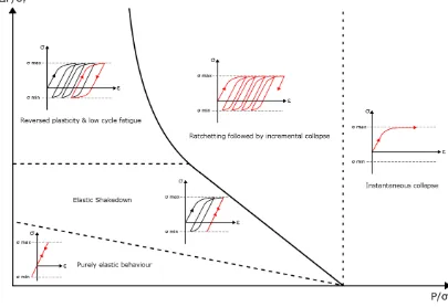
In addition to understanding the fatigue life of engineering components, the ability to predict the precise load at which failure will occur is also vitally important in order to ensure their integrity during operational life. For this reason, a thorough understanding of different failure behaviours is crucial both in the component design stage and also during service for condition monitoring purposes. Under cyclic loading, engineering structures can experience a number of different material responses, depending upon the applied load level. These can include purely elastic behaviour, elastic shakedown, reversed plasticity, ratcheting and instantaneous collapse. Understanding the load ranges at which these conditions will occur can aid in the development of engineering components, since damaging behaviour can be avoided through careful design. Ratcheting and instantaneous collapse must be avoided for obvious reasons. However, small amounts of plasticity can be tolerated, provided that it shakes down to fully reversed plasticity or elastic shakedown, since at these loads, continued incremental plasticity and ultimate failure will not occur under repeated loading.

4 important information about the failure mechanisms of the component can be deduced. This will then aid in the prediction of the failure modes of the engineering structure. For this reason, it is not uncommon to deliberately design a test specimen to fail within a certain life. Fracturing a specimen during experimental testing in a safe, controlled environment provides important information about the failure mechanisms that can occur in the final component, meaning that its design can be adapted if necessary to suit the operating conditions of the engineering structure. This type of testing is prominent in a number of different industries, but is of particular importance in the development of industrial gas turbines, which is the focus of this investigation. This paper concerns the prediction of shakedown and ratcheting failure modes within an experimental test specimen which is representative of gas turbine nozzle guide vanes.

1.2 Linear Matching Method

The analysis of the steady state response of engineering structures provides invaluable information about the integrity of components when subject to cyclic loading. Few analytical methods exist for this type of investigation and numerical Finite Element modelling can provide much needed information. This steady state response can be calculated with the use of extensive FE modelling in which every cycle is simulated in a separate step of the analysis, this is referred to as a step-by-step analysis. In order to achieve a steady state response, a large number of cycles are required and as a result complete modelling in this way is very computationally expensive and time consuming. This is discussed in greater detail in Section 1.4. Although the increase in computing power in recent years has made this type of analysis more feasible, they cannot always conclusively determine the material response and cannot ascertain the proximity to the limit. Direct cyclic analysis (DCA) methods provide an alternative method of determining the steady state shakedown and ratchet response of structures. A key advantage of these techniques over step-by-step analyses is that full details of the entire load history are not required and instead, only the most dominant loads acting on the structure are required. This leads to significantly reduced computational expense and analysis times, whilst still maintaining a comparable level of accuracy to step-by-step FE methods [18].

5 Due to the power of the LMM, it has been part of the R5 research programme for a number of years [28, 31] and is routinely used by EDF for the structural analysis of many nuclear power plant components [39, 40]. However, despite the major advantages of the LMM, its use is not widespread and is still fairly uncommon outside of the work of EDF.

The LMM process aims to replicate a non-linear, elastic plastic material response through the modification of a series of linear elastic analyses. Initially the material and loading properties are defined and a linear elastic analysis is performed. The LMM then modifies the modulus at each node in the structure so that the induced stress matches the yield stress of the material. An additional linear elastic analysis is then performed using these modified values of modulus. This causes the stresses to redistribute throughout the structure. This process repeats iteratively, continually modifying the modulus until the stress throughout the structure redistributes to match that of an elastic-plastic material response.

1.3 Bree Interaction Diagram

[image:6.595.91.496.167.445.2]

6 Through reference with the Bree-like interaction diagram, the LMM method can very efficiently determine the limit boundaries of each of these damage mechanisms by calculating the precise loads at which they occur. It also allows the assessment of intermediate loads by ascertaining what type of behaviour will occur at a given applied load. This makes it a very powerful technique for the damage assessment of engineering components.

Figure 1: Bree interaction diagram showing stress-strain responses at each region

1.4 Fatigue Life Assessment Methods

The ability to determine the lifetime of a component is vitally important and there exist a number of fatigue life assessments that offer efficient methods of estimating the number of cycles to failure of an engineering component. The Neuber Correction Method [46-50] is one of the most commonly known methods and is widely used in industry for fatigue life assessment [51, 52]. This is a strain based life assessment method that is approximated from a purely elastic solution. A linear elastic analysis is performed and the induced behaviour at a stress concentration is calculated. The strain life method requires true stresses and strains and so the elastic solution is adjusted to allow for local plasticity. Thus, a correction is applied to compensate for the elastic solution and to approximate deformation. The stress range and strain range can then be predicted from this modified solution. Since this method is based on the stress concentration and the induced strain range, it is sensitive to the material properties under investigation. This method is also highly conservative, however, in highly technical industries such as the power industry, due to the safety implications involved, this level of conservatism is often required.

7 implications of engineering components, since a greater understanding of the fatigue life of the structure is gained.

It is possible to manually determine the limit boundaries and thus determine the structural response manually through a series of step-by-step analyses. However, this cannot directly predict the location of the limit boundaries and can only indicate the type of structural response that occurs at a given load, whether it is instantaneous collapse, ratcheting, reversed plasticity or shakedown. Therefore, since the position of the boundaries is not known, the process is entirely trial and error and is incredibly time consuming and computationally intensive. Numerous analyses would need to be run and their strain history response monitored. The user would then need to modify the applied loading and rerun the analysis, continually refining the position of the boundaries in an iterative manner. For this reason, this is clearly not a viable option for determining the location of the limit boundaries. However, it can provide a very useful method of verification if the position of the boundary is already known. Performing a small number of step-by-step analyses above and below the limit boundary lines and monitoring their strain response can verify the accuracy of the limits.

1.5 Objectives

The objective of this investigation is to design an experimental testing programme which is sufficient for causing crack initiation in a complex notched specimen. The shakedown and ratchet limits will be calculated with reference to the Bree interaction diagram, to allow the calculation of the range of loads that will induce crack initiation. A low cycle fatigue analysis will then be performed to select an appropriate design load from this suitable range, which best suits the fatigue requirements of the test. The structure of this paper is organised as follows: Section 1 above has explained the rationale of this investigation, and the importance of careful design of experimental test specimens has been highlighted. In Section 2, a new method is proposed for the design of an experimental testing programme. The basis of this and the background theory of the LMM are then introduced in reference to the fundamental shakedown and ratchet theorems. In Section 3, a description of the problem is provided and the precise geometry of the bespoke test specimen and the material properties and loading conditions are described. A description of the finite element model that is used in the analysis is also included. Section 4 presents the obtained results of the shakedown and ratchet boundary limits which allows the determination of an appropriate design load range. In order to assess the accuracy of the results, the analysis convergence is investigated and the results are verified through a step-by-step analysis. Finally, in Section 5, a low cycle fatigue analysis is performed and an appropriate specific design load is chosen based on the obtained results in Section 4, with consideration of the likely location of crack initiation. The paper concludes with a discussion of the arrangement of the experimental test that will be performed as a result of this investigation and a consideration of future works.

2. Numerical Procedure

2.1 Reversed Plasticity Domain Method

8 paper as the Reversed Plasticity Domain Method (RPDM). It comprises a series of Linear Matching Method analyses for the precise calculation of the shakedown and ratchet limit boundaries in order to identify the reversed plasticity and low cycle fatigue region, in which crack initiation will occur. A Bree-Interaction diagram can then be plotted for visualisation of the critical regions. Identification of this zone allows the calculation of the range of loads in which reversed plasticity and crack initiation will occur. A low cycle fatigue analysis can then be performed which calculates the number of cycles to crack initiation for all loads within this range. The user may then select a single specific design load based on the fatigue life requirements of the component. The Reversed Plasticity Domain Method provides a suite of analysis tools to provide a very efficient technique that encompasses the identification of loads ranges for causing specific damage mechanisms as well as the calculation of the low cycle fatigue life for crack initiation. An optional step-by-step analysis can then be performed as a means of verification if required. This investigation applies this new technique to a complex industrial problem, clearly demonstrating its power and efficiency for the design of experimental testing programmes.

The crack initiation assessment is associated with low cycle fatigue, hence it is possible to use LCF material data to assess the lifetime from the steady state cycle strain range data. The calculation of the plastic and total strain range is performed through the first stage of the ratchet analyses of the LMM Direct Steady Cyclic Analysis (DSCA). This is a standalone component of the Linear Matching Method which obtains the steady cyclic stresses and strain rates for given combinations of loading through an iterative procedure which directly locates the ratchet limit [53]. This is explained further in Section 2.3.

It is important to note that this procedure only considers the calculation of the number of cycles to crack initiation and does not consider crack propagation life. Additional analyses would need to be performed to model crack propagation. However, for the current alloy, the time for crack propagation is much shorter than the time for crack initiation. It is believed that for this investigation, the initiation fatigue life is sufficient for designing the experimental testing programme. The aim of this research is to calculate the appropriate cyclic load levels which induce crack initiation within a predefined number of cycles. The objective is to determine, using the proposed method, the cyclic load level that causes the crack to initiate.

2.2 Shakedown Theorems

The shakedown and ratchet calculations performed as part of the RPDM are done by the Linear Matching Method. The precise methodology of this is thoroughly described in existing literature. The shakedown theorems are clearly explained by the work of Ponter [54] and this is briefly outlined below. It states that the shakedown limit can be described as the range of the load multiplier,

S

λ λ

≤

for a residual stress change of zero, where

λ

S is the shakedown limit and the residual stress is denoted as r

ij

9 Upper Bound Theorem

The upper bound theorem is based on Koiter’s theorem [55, 56], which states that “a structure under cyclic loadings would shakedown if the external work done by the loads is less than or equal to the internal work dissipated for all admissible strain rate cycles, c

ij

ε



_.”

Assuming an isotropic, elastic perfectly plastic material that satisfies the Von Mises yield condition, the problem comprises a 3D body of volume, V , with a boundary, S, that experiences a cyclic mechanical loading history

λ

P x t_i( _j, ) on

S

_T and a temperature load of

λθ

(x t_j, ) within

volume V , over a cycle time period ∆t.

λ

is a load parameter and

u

i

=

0

is the displacement rate

that is applied on

S

U.

S

T and

S

U are sections of the boundary, S. The basis of the method is that the admissible and incompressible strain rate history, c

ij

ε



_{, is associated with a compatible strain} increment, c

ij

ε

∆

, such that:

∫

∆

∆

=

t c ij c ij

dt

0

ε

ε



(1)

where the strain increment is associated with a displacement increment field, given by:

)

(

2

1

i c j j c i c ij

x

u

x

u

∂

∆

∂

+

∂

∆

∂

=

∆ε

(2)

From the load history as above, the upper bound shakedown theorem is then given by:

∫ ∫

∫ ∫

∆

=

∆

=

V t c ij c ij V t c ij ij

UB

dtdV

dtdV

0 0

)

(

)

ˆ

(

σ

ε

σ

ε

λ





(3)

where c ij

σ

is the stress at the yield and is associated with c ij

ε



and

σ

ˆijis a linear solution associated with the given load history [28, 57].

λ

UB ≥

λ

S is an upper bound to the shakedown load parameter,

S

λ

. This can be further simplified to give:

∫ ∫

∫ ∫

∆ ∆

=

V t c ij ij V t c ij y UB

dtdV

dtdV

0 0

)

ˆ

(

)

(

ε

σ

ε

ε

σ

λ







(4)

Where

σ

y is the temperature-dependent yield stress of the material,

ε

ijis a kinematically admissible strain rate and

ε



ε



ij

ε



ij

3

2

10 Lower Bound Theorem

In the shakedown condition, by definition, no plastic strain will accumulate when the combination of elastic stresses and residual stress field satisfy the von Mises yield criterion. The lower bound theorem states that shakedown will occur if a time independent residual stress field exists which satisfies the equilibrium and boundary conditions and the total stress is less than the yield limit. This is based on Melan’s Theorem [56, 58] which states that “if a time constant residual stress field,

ρ

ij( )x exists such that superposition with induced elastic stresses,

λ σ

LB ˆ ( , )ij x t forms a

safe state of stress everywhere in the structure, i.e.

ˆ

( LB ij( , ) ij( )) 0

f

λ σ

x t +

ρ

x ≤ (5)

then

λ

_LB

≤

λ

_S” where

λ

LBis the lower bound parameter. This utilises a similar iterative process as above in which a convergent lower bound value of the shakedown limit is calculated.

2.3 Ratchet Theorems

The theorem for the ratchet limit analysis is based on an extension of the shakedown theorems, where the change of accumulated residual stress field,

ρ

ij( )tn at time instance

t

n, is included in the linear elastic solution. This is explained by Chen et al [31, 59]. The first step of the analysis involves the evaluation of the changing residual stress field,

ρ

ijr

( , )

x t

and plastic strain ranges. Within the

Linear Matching Method framework, this is referred to as the Direct Steady Cycle Analysis (DSCA). This iteratively calculates the varying residual stress,

∆

ρ

_ijr

( , )

x t

_{n m}, associated with the elastic solution,

σ

ˆ ( , )

_ij∆

x t

_n , where

n

is the cycle number. This repeats iteratively from cycle n=1 until convergence is reached at cycle n=M. Using the obtained values of the residual stress history and plastic strain ranges at a time point,

t

n, the second step of the analysis then performs the traditional shakedown procedure, as explained above, to assess the ratchet limit. As previously demonstrated in equations (1) and (3), the upper bound shakedown theorem can be given by:

∫ ∫

∫ ∫

∆

=

∆ V t c ij c ij V t c ij c ij

UB

dtdV

dtdV

0 0

)

ˆ

(

σ

ε

σ

ε

λ





(6)

where:

ˆ

_ij

ˆ

_ijF

ˆ ( , )

_ij

x t

_{k ij}r

(

x t

_k

, )

σ

₌

λσ

₊

σ

∆

₊

ρ

₍₇₎

Defining the von Mises yield condition with the associated flow rule, gives the upper bound ratchet limit multiplier,

λ

UB, subject to a cyclic load history,

σ

ˆ ( )

ij

t

n

∆ _{and an additional applied constant}

load,

ˆ

F ij

σ

, as:

1 1

1

ˆ

( ) ( ( ) ( ))

ˆ ( )

N n N n

n y ij n ij n ij n ij

V V

UB _{F N n}

ij n ij V

dV t t dV

dV

σ ε ε

σ

ρ

ε

λ

σ

ε

∆ = = = ∑ ∆ − ∑ + ∆ = ∑ ∆

∫

∫

11

where

(

)

2

3

n n n

ij ij ij

ε ε

∆

=

∆ ∆

ε ε

and n ij

ε

∆

is the kinematically admissible plastic strain rate history.

Based on this, the LMM then produces a sequence of monotonically reducing upper bounds and converges to the least upper bound ratchet limit [59].

The algorithms iteratively compute the shear modulus, Jacobian matrix, residual stress and modified stress. This allows the user to perform a complete analysis to calculate the shakedown and ratchet limits as well as other important cyclic information such as strain range for use in LCF analysis. These theorems are embedded into the Linear Matching Method code and ABAQUS plugin[36-38]. The user-friendly environment of the plugin means that these parameters can be calculated without the need to completely understand the theoretical background. This demonstrates the power of the LMM ABAQUS plugin as an ergonomically well designed and user friendly software tool.

3. Numerical Application

3.1 Description of the Problem

12

3.2 Test Specimen Geometry

[image:12.595.116.479.144.437.2]

In order to address the requirement for a representative component for the assessment of nozzle guide vanes, the proposed test specimen comprises a cylindrical bar with scalloped edges, containing a chamfered through hole as shown in Figure 2.

Figure 2: Drawing of test specimen geometry

3.3 Material Properties & Loading Conditions

A nickel based super alloy, similar to those used in turbine applications is used in this investigation with a Young’s Modulus of 178 GPa and yield stress of 648 MPa. The Linear Matching Method Direct Steady Cyclic Analysis (DSCA) procedure can accurately model elastic perfectly plastic materials. However, in addition, it is able to consider material hardening/softening through the inclusion of the Ramberg-Osgood (RO) formula. This matches the inclusion of hardening/softening in the R5, allowing it to work harmoniously with this procedure. This allows the LMM DSCA to be used on a wide range of material models, matching the requirements of real components very accurately if required, or on more simple cases if elastically perfectly plastic models are sufficient, which reduces the computational time. For materials that exhibit small levels of hardening, elastic perfectly plastic (EPP) properties offer simplified material models which can still provide reasonable levels of accuracy. In this investigation, both EPP and RO material models are analysed and a comparison between the two is offered. This allows the impact that material hardening has on the fatigue life of a component to be demonstrated. The Ramberg-Osgood model that is adopted in this investigation follows the relationship:

β

σ

σ

ε

1

)

2

(

2

2

E

A

13 where,

ε

Tis the total strain range, ∆

σ

is the cyclic stress range,

E

is the multi-axial Young’s Modulus and A=1175MPa and

β

=0.068 are material constants.

[image:13.595.88.505.224.305.2]

In the LMM plugin, the user specifies an arbitrary applied reference load and loading history. The LMM then calculates the shakedown or ratchet limit multiplier as a fraction of this reference load, i.e. if a reference load of 100 MPa is applied and a shakedown limit multiplier of 0.5 is yielded, then the shakedown limit would be 50MPa. In this investigation, a reference load of magnitude 400 MPa is applied to one end of the specimen, whilst the opposite end is pinned in position to prevent movement, as illustrated in Figure 3.

Figure 3: Applied loading conditions

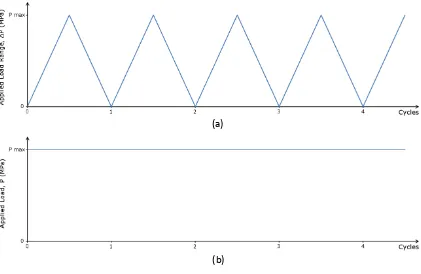
In Bree’s original case of a thin walled cylinder, a static mechanical load and cyclic thermal loads were applied. The industrial test in this investigation is to be performed with cyclic mechanical loading under isothermal conditions. The constant temperature field means that no thermal stress concentrations will be induced, meaning that there is no primary thermal load to apply. Therefore, instead of a thermal and mechanical load, two separate mechanical loads are applied to the test specimen. Each load will be of identical magnitude, however, one will be kept static, whilst the other is cycled. The loading history applied in this investigation is illustrated in Figure 4.

Figure 4: Loading history for (a) cyclic load and (b) static load

(a)

[image:13.595.77.498.458.732.2]

14 The application of independent static and cyclic mechanical loads means that the generated Bree-like interaction diagram provides information for the entire range of R-ratios since the cyclic and static loads are plotted independently on separate axes. Monitoring the response at varying values of the static load (x-axis), allows the material response at different R-ratios to be ascertained. For this investigation, an R-ratio of zero is required which corresponds to the Y-axis, at x=0.

3.4 Finite Element Model

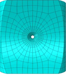
[image:14.595.143.453.317.547.2] [image:14.595.231.366.585.741.2]

The finite element software package, ABAQUS is used for the computational analyses performed in this investigation. Within ABAQUS, the proposed test specimen as presented in Figure 2 is modelled. The central region of the model containing the chamfered centre hole is modelled using quadrilateral hexahedral elements and the ends of the specimen are modelled with quadrilateral tetrahedral elements. This allows the implementation of a refined mesh around the most critical regions of the specimen, whilst a more coarse mesh is used in the less critical regions, thus reducing the computational expense of the analyses. The mesh that is used in this investigation is shown in Figure 5 and an enlarged view of the mesh around the centre hole shown is in Figure 6.

Figure 5: Model mesh showing different element types used

Figure 6: Mesh of the central region of model

2nd _{order tetrahedral}

15

4. Numerical Results

4.1 Shakedown & Ratchet Limit Boundaries

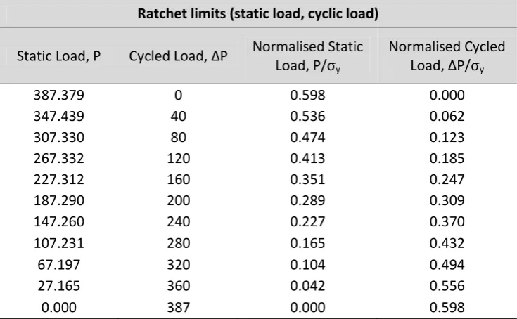
The RPDM is used to perform a number of shakedown and ratchet analyses which allows the shakedown and ratchet boundary conditions to be calculated. These results are shown in Table 1 and Table 2; P and ΔP are the magnitudes of the static and cycled loads respectively and P/σy and ΔP/σy are P and ΔP normalised with respect to the yield stress of the material.

Shakedown limits (static load, cyclic load)

Static Load, P Cycled Load, ΔP Normalised Static _{Load, P/σy} Normalised Cyclic _{Load, ΔP/σy}

0.000 231.084 0.000 0.357

23.108 231.075 0.036 0.357

46.213 231.064 0.071 0.357

69.310 231.035 0.107 0.357

92.300 230.749 0.142 0.356

115.375 230.749 0.178 0.356

145.234 242.057 0.224 0.374

[image:15.595.113.483.193.376.2]

387.302 0.000 0.598 0.000

Table 1: Shakedown limits calculated by the LMM

Ratchet limits (static load, cyclic load)

Static Load, P Cycled Load, ΔP Normalised Static _{Load, P/σy} Normalised Cycled _{Load, ΔP/σy}

387.379 0 0.598 0.000

347.439 40 0.536 0.062

307.330 80 0.474 0.123

267.332 120 0.413 0.185

227.312 160 0.351 0.247

187.290 200 0.289 0.309

147.260 240 0.227 0.370

107.231 280 0.165 0.432

67.197 320 0.104 0.494

27.165 360 0.042 0.556

0.000 387 0.000 0.598

Table 2: Ratchet limits calculated by the LMM

[image:15.595.114.482.408.635.2]

16

[image:16.595.79.548.85.372.2]

Figure 7: Shakedown-Ratchet limit boundaries

Since the aim of this investigation is to determine the loads required to cause crack initiation, the area of interest on the shakedown-ratchet Interaction diagram is the reversed plasticity region, as highlighted in red in Figure 7, where the x-axis corresponds to the static load and the y-axis corresponds to the cyclic load. However, in the experimental test, an R-ratio of zero is required and no static load is to be applied, meaning that the only region of interest for calculating the required load range is at x=0. It can be seen that at x=0, the shakedown and ratchet limits are 0.357 and 0.598 respectively. These values are normalised with respect to the yield stress and so when corrected become 231.336 MPa and 387.504 MPa. Therefore, the limit loads can be summarised as shown in Table 3. A series of step-by-step analyses are performed as a means of verification for the results generated using the RPDM and these are presented in Section 4.3. Due to the nature of the mechanical load and the fact that there is no thermal load, the ratchet limit coincides with the limit load and so in this particular case, there is no visible ratchetting region as any load larger than the ratchet limit load will cause instantaneous collapse.

ΔP/σy Load (MPa)

Shakedown Limit 0.357 231.336

[image:16.595.160.433.619.662.2]

Ratchet Limit 0.598 387.504

Table 3: Shakedown and ratchet limit loads for the load condition of R=0

4.2 Convergence Investigation

In order to ascertain the accuracy of the obtained solution from the RPDM LMM analysis, it is important to consider the convergence rate. In the LMM plugin for ABAQUS CAE as part of the RPDM, the desired convergence rate can be specified as either the difference between consecutive upper bounds, or the percentage difference between upper bounds and lower bounds. As a general

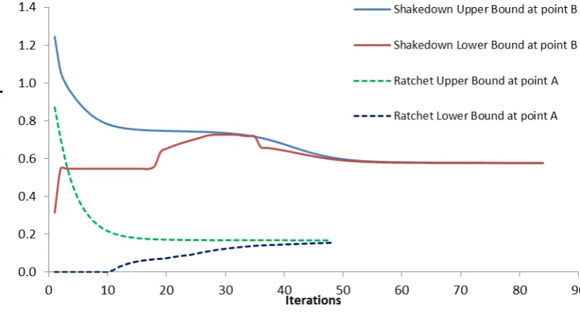
17 case, the upper bound solution converges more quickly than the lower bound [28] and so is often the preferable choice of convergence criteria. During each iteration of the analysis, the upper and lower bounds of the shakedown or ratchet load multiplier are calculated. The solution is deemed to have converged once the user defined convergence criteria have been satisfied. In order to assess that the convergence is satisfactory, a load condition was selected from both the shakedown and ratchet regimes as indicated by the letters A and B in Figure 7 and the respective load multiplier is plotted at each increment as shown in Figure 8.

[image:17.595.100.513.469.691.2]

At load point A, the ratchet analysis reaches convergence fairly quickly, with the upper bound converging in approximately 20 iterations whilst the lower bound takes slightly longer, reaching convergence in approximately 47 iterations. However, at load point B, the shakedown analysis experiences a peculiar phenomenon. The upper bound reaches an initial steady state in approximately 15 iterations, however, whilst the lower bound is approaching convergence, at iteration 32, the LMM detected a change in the failure mechanism and the upper bound started to re-converge on the limit multiplier of this new failure mechanism. This caused the upper bound shakedown limit multiplier to drop below that of the lower bound multiplier. Such a situation would cause numerical errors and so in response, the LMM automatically changes the convergence criteria to be based solely on the upper bound. The analysis then continued, reaching final convergence in approximately 55 iterations. This highlights the importance of monitoring both the upper bound and lower bound limit loads since each solution can be validated against one another, giving greater confidence in their accuracy [60]. If only one condition is used as convergence criteria, then it could be possible to miss a failure mechanism, yielding inaccurate and incomplete results. Monitoring both lower and upper bounds that tend towards a common solution in this way is one of the major strengths of the Linear Matching Method and it makes convergence generally faster, more stable and more accurate than other methods [33].

18

4.3 Verification of Results

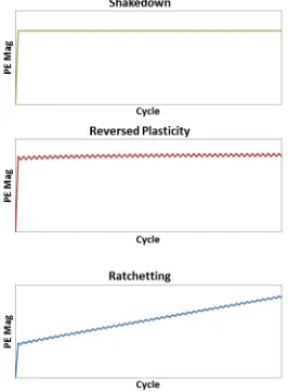
[image:18.595.175.441.385.746.2]

The accuracy of the RPDM can be verified by performing a series of standard step-by-step analyses at different regions of the Shakedown-Ratchet Boundary diagram and monitoring the strain magnitude history data. Each type of damage behaviour exhibits a different strain response and through monitoring this, the accuracy of the location of the boundaries can be determined. For a material with elastic-perfectly plastic properties, the shakedown strain response increases linearly to a critical value, at which points it remains constant, producing a bilinear curve. Under reversed plasticity, the strain again initially increases linearly, but on reaching a critical point, oscillates about a mean value. Under ratcheting conditions, the strain continuously increases until eventual collapse occurs. These strain responses are illustrated in Figure 9. Observation of these responses can indicate the location of the boundaries. If at a particular load point, shakedown occurs but at a slightly increased load, reversed plasticity occurs, then it can be deduced that the limit boundary occurs between these two load points. To assess this, six analyses of 100 cycles each were performed at points above and below the shakedown and ratchet boundaries as illustrated by the crosses in Figure 10. This demonstrates the Shakedown-Ratchet Boundary plots with the strain magnitude response superimposed. The crosses show the load points at which step-by-step analyses were performed. It clearly shows that the observed strain response accurately matches the damage behaviour, thus proving the accuracy of the RPDM results for the shakedown and ratchet boundaries.

[image:19.595.78.539.67.419.2]

19

Figure 10: Step-by-step analysis verification of shakedown and ratchet boundaries

Following successful verification of the RPDM results by step-by-step analyses, it can be concluded that a load range of between 231 MPa and 387 MPa will cause crack initiation. In order to determine the most appropriate load between these ranges, a low cycle fatigue analysis is now required.

5 Evaluation & Discussion

5.1 Low Cycle Fatigue Assessment

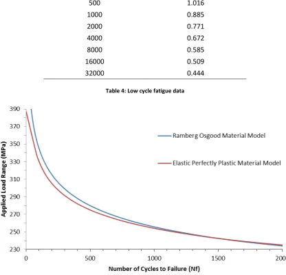
20 Number of Cycles to Failure Normalised Strain Range (%)

100 1.400

500 1.016

1000 0.885

2000 0.771

4000 0.672

8000 0.585

16000 0.509

[image:20.595.149.447.72.233.2]

32000 0.444

[image:20.595.86.503.120.519.2]

Table 4: Low cycle fatigue data

Figure 11: Number of cycles to failure with increasing applied cyclic load range for R-ratio of 0 using

The variation of LCF life to crack initiation for varying applied loads can clearly be seen for both EPP and RO material models. As the load increases, this fatigue life decreases until the limit load is reached, where the specimen will instantaneously collapse on the first load cycle. Below the shakedown limit, the applied load is less than the low cycle fatigue limit of the specimen and so low cycle crack initiation will never occur. It can be seen that using the EPP material model, the calculated fatigue life is lower than that of the RO model, calculating a potentially overly-conservative, and unrealistic value of the total LCF life.

21 is considered optimum since it is above the shakedown limit, ensuring that cracking occurs, yet it has a relatively long low cycle fatigue life of approximately 650 cycles to crack initiation. This will allow sufficient time to observe the necessary data that will be obtained during the test. This is

[image:21.595.179.418.152.262.2]

summarised in Table 5.

Material Model

EPP RO

Stress Range (MPa) 1296.00 1330.68 Elastic Strain Range (%) 0.7329 0.7483 Plastic Strain Range (%) 0.2436 0.2115 Total Strain Range (%) 0.9764 0.9598

LCF Life (cycles) 603 658

Table 5: Stress and strain ranges calculated using both Elastic Perfectly Plastic and Ramberg-Osgood Material Models and corresponding fatigue life calculated by the RPDM

Both the Ramberg-Osgood (RO) and Elastic Perfectly Plastic (EPP) material models are included to demonstrate the effect that the material hardening has on the fatigue life. It can clearly be seen that the elastic strain range for the RO model is larger than EPP, whilst the plastic strain range for the RO model is smaller than for EPP. This results in a smaller total strain range for the RO model, yielding a longer life than for EPP. This matches the typical response that is expected for such material models, and highlights the importance of implementing realistic material models which include cyclic hardening for a thorough and accurate prediction of low cycle fatigue life. However, it can be seen that in this particular case, the absolute effect on the LCF life is relatively small.

[image:21.595.292.512.497.716.2]

For the chosen load of 270MPa, the steady state hysteresis loops are plotted in Figure 12 and Figure 13. These confirm that the mechanism undergoes a reversed plasticity response at an applied load of this magnitude. The difference in total stress and strain ranges can also clearly be seen.

Figure 12: Stabilised hysteresis loop at applied load of

[image:21.595.76.288.500.706.2]

22

5.2 Arrangement of Experimental Test Specimen

[image:22.595.100.497.223.453.2]

In addition to predicting the number of cycles to failure, it is important to consider the point of crack initiation. Figure 14 shows the induced total strain range under loading for both EPP and RO material models. The points of maximum stress are clearly very localised at the edges of the centre hole and are likely locations of crack initiation. Due to the symmetry of the specimen, the strain at each side of the centre hole on each face is of similar magnitude and so the exact location of initiation is unknown as it could be at one of four locations. This poses a potential issue for experimental testing but in order to ensure that crack initiation is witnessed, each face of the specimen must be monitored.

Figure 14: Total strain range induced at stress concentration under cyclic loading for Elastic Perfectly Plastic (a) and Ramberg-Osgood (b) Material Models

It is important to note that the contour plots shown in Figure 14 are calculated using the nodal values, however, for the LCF analysis above, the stress and strain values are calculated at the most critical integration point in the most critical element. As a result, the values calculated by ABAQUS at the node locations are slightly higher than at the integration point. This figure is intended for illustrative purposes to demonstrate the location of crack initiation, and not for an in depth LCF analysis.

[image:23.595.128.474.84.263.2]

23

Figure 15: Machined industrial test specimen

The scope of the testing is to perform 10 tests, comprising three series: (1) Simple fatigue cycle

(2) Initial single tensile overload cycle followed by simple fatigue cycle (3) Initial single compressive overload cycle followed by simple fatigue cycle

Three specimens would be tested for each series of test conditions with the tenth specimen considered a spare, and will either be tested based on the outcome of the other 9 tests, or used as a trial run. All tests will be load controlled and conducted at R=0 under isothermal conditions at 500°C with an applied load range of 270 MPa. For the case of the overload, this is to be 25% higher than the normal fatigue cycle load, i.e. 337.5 MPa. The purpose of these tensile and compressive overloads is to create a residual stress field in the notch in order to observe the effect this has on the structural integrity of the component.

During the tests, crack initiation and propagation will be measured using DC (direct current) potential drop monitoring. This is a non-destructive examination technique that applies a constant direct current to the specimen and measures the induced resistance. Any change in the geometry through cracking will induce a change in resistance. Through correct calibration, this change in resistance can be related to crack growth [61]. To allow implementation of this technique during the testing of the specimen, measurement probes are installed either side of the central hole and a reference probe is installed away from the stress concentration for comparison purposes. This will allow the change of resistance induced in the specimen as the crack grows and its initiation and extension to be measured. These probes will be positioned outside the centre hole so as to avoid potentially influencing the results of the test.

24

5.3 Future Work

This investigation has demonstrated the power and efficiency of the use of the Reversed Plasticity Domain Method for the design of an industrial test specimen. However, this has only considered an alternating load history with no regard for extended hold times or cyclic thermal loading. Engineering structures in gas turbine applications often undergo extended hold times at elevated cyclic temperature loading, and thus creep and thermo-mechanical fatigue (TMF) can be prominent failure mechanisms. For this reason, the consideration of creep and TMF in the design of components is vitally important. To this end, the design of an experimental testing programme with the inclusion of extended hold times in the cyclic loading condition, as well as TMF loading, will be the focus of future investigations. The results for both an alternating load history and alternating load with extended hold times will then be compared to experimental results in order to gain a better understanding of the failure behaviour and to assess the accuracy of these results.

6. Conclusions

The Reversed Plasticity Domain Method has been proposed as a technique for the design of an experimental testing programme suitable for causing crack initiation in a complex notched specimen through the calculation of the shakedown and ratchet limits. The shakedown limit and ratchet limit loads have been identified as 231MPa and 387MPa respectively and as such, any load between these values is sufficient to cause low cycle fatigue crack initiation. The accuracy of the results obtained using the RPDM has been verified through inspection of the strain range history data of a series of step-by-step analyses. Following successful verification, a strain based low cycle fatigue analysis was performed in order to calculate the number of cycles to crack initiation for a range of loads between the shakedown and ratchet limits. This allowed an optimum design load to be determined which meets the requirements of the test within the imposed time constraints. Following a complete low cycle fatigue analysis, a design load of 270 MPa has been selected as the optimum load for the experimental test. This load yields a fatigue life of approximately 658 cycles to crack initiation for a Ramberg-Osgood material model and 603 cycles for an Elastic Perfectly Plastic material model. The location of likely crack initiation has also been identified. The experimental procedure that will be performed as a result of this investigation has been discussed with a detailed description of each test provided. Finally, future work that follows on from this study has been suggested.

This investigation clearly demonstrates the power and efficiency of the Reversed Plasticity Domain Method and the Linear Matching Method for the calculation of the shakedown and ratchet limits as well as the design of an experimental testing programme and LCF analysis for a highly complex industrial test specimen.

Acknowledgements

25

References

1. Sachs, N.W., Practical plant failure analysis: a guide to understanding machinery deterioration and improving equipment reliability. 2006: CRC Press. 57.

2. Paris, P.C., M.P. Gomez, and W.E. Anderson, A rational analytic theory of fatigue. The trend in engineering, 1961. 13(1): p. 9-14.

3. Dowling, N.E., Fatigue failure predictions for complicated stress-strain histories. 1971, DTIC Document.

4. Brown, M. and K. Miller, A theory for fatigue failure under multiaxial stress-strain

conditions. Proceedings of the Institution of Mechanical Engineers, 1973. 187(1): p. 745-755.

5. Bush, S., Failure mechanisms in nuclear power plant piping systems. Journal of pressure vessel technology, 1992. 114(4): p. 389-395.

6. Schütz, W., A history of fatigue. Engineering fracture mechanics, 1996. 54(2): p. 263-300. 7. Farfan, S., et al., High cycle fatigue, low cycle fatigue and failure modes of a carburized

steel. International journal of fatigue, 2004. 26(6): p. 673-678.

8. Liu, Y., et al., Prediction of the S–N curves of high-strength steels in the very high cycle fatigue regime. International journal of fatigue, 2010. 32(8): p. 1351-1357.

9. Chan, K.S., Roles of microstructure in fatigue crack initiation. International Journal of Fatigue, 2010. 32(9): p. 1428-1447.

10. Morishita, T. and T. Itoh, Evaluation of multiaxial low cycle fatigue life for type 316L stainless steel notched specimen under non-proportional loading. Theoretical and Applied Fracture Mechanics, 2016.

11. Shi, K., et al., A prediction model for fatigue crack growth using effective cyclic plastic zone and low cycle fatigue properties. Engineering Fracture Mechanics, 2016.

12. Lin, Y., et al., Investigation of uniaxial low-cycle fatigue failure behavior of hot-rolled AZ91 magnesium alloy. International Journal of Fatigue, 2013. 48: p. 122-132.

13. Kamaya, M., Low-cycle fatigue crack growth prediction by strain intensity factor. International Journal of Fatigue, 2015. 72: p. 80-89.

14. Li, H., H. Yuan, and X. Li, Assessment of low cycle fatigue crack growth under mixed-mode loading conditions by using a cohesive zone model. International Journal of Fatigue, 2015.

75: p. 39-50.

15. Rabbolini, S., et al., Crack closure effects during low cycle fatigue propagation in line pipe steel: An analysis with digital image correlation. Engineering Fracture Mechanics, 2015.

148: p. 441-456.

16. Chen, G., et al., Low cycle fatigue and creep-fatigue interaction behavior of nickel-base superalloy GH4169 at elevated temperature of 650° C. Materials Science and Engineering: A, 2016. 655: p. 175-182.

17. Deng, J., et al., Research on CTOD for Low-Cycle Fatigue Analysis of Central-through Cracked Plates Considering Accumulative Plastic Strain. Engineering Fracture Mechanics, 2015.

18. Lytwyn, M., H. Chen, and M. Martin, Comparison of the Linear Matching Method to Rolls-Royce's Hierarchical Finite Element Framework for ratchet limit analysis. International Journal of Pressure Vessels and Piping, 2015. 125: p. 13-22.

19. Ponter, A.R. and M. Engelhardt, Shakedown limits for a general yield condition: implementation and application for a von Mises yield condition, in Inelastic Analysis of Structures under Variable Loads. 2000, Springer. p. 11-29.

20. Ponter, A.R., A linear matching method for shakedown analysis. 2002: Springer.

21. Ure, J., H. Chen, and D. Tipping, Verification of the Linear Matching Method for Limit and Shakedown Analysis by Comparison With Experiments. Journal of Pressure Vessel Technology, 2015. 137(3): p. 031003.

26

23. Muscat, M., D. Mackenzie, and R. Hamilton, Evaluating shakedown under proportional loading by non-linear static analysis. Computers & structures, 2003. 81(17): p. 1727-1737.

24. Seshadri, R., The generalized local stress strain (GLOSS) analysis—theory and applications. Journal of pressure vessel technology, 1991. 113(2): p. 219-227.

25. Malena, M. and R. Casciaro, Finite element shakedown analysis of reinforced concrete 3D frames. Computers & Structures, 2008. 86(11): p. 1176-1188.

26. Casciaro, R. and G. Garcea, An iterative method for shakedown analysis. Computer methods in applied mechanics and engineering, 2002. 191(49): p. 5761-5792.

27. Chen, H., A.R. Ponter, and R. Ainsworth, The linear matching method applied to the high temperature life integrity of structures. Part 1. Assessments involving constant residual stress fields. International Journal of Pressure Vessels and Piping, 2006. 83(2): p. 123-135.

28. Chen, H., Lower and upper bound shakedown analysis of structures with temperature-dependent yield stress. Journal of Pressure Vessel Technology, 2010. 132(1): p. 011202. 29. Chen, H., W. Chen, and J. Ure. A direct method on the evaluation of cyclic behaviour with

creep effect. in ASME 2012 Pressure Vessels and Piping Conference. 2012. American Society of Mechanical Engineers.

30. Chen, H. and A.R. Ponter, A method for the evaluation of a ratchet limit and the amplitude of plastic strain for bodies subjected to cyclic loading. European Journal of Mechanics-A/Solids, 2001. 20(4): p. 555-571.

31. Chen, H. and A.R. Ponter, A direct method on the evaluation of ratchet limit. Journal of Pressure Vessel Technology, 2010. 132(4): p. 041202.

32. Ponter, A.R. and H. Chen, A minimum theorem for cyclic load in excess of shakedown, with application to the evaluation of a ratchet limit. European Journal of Mechanics-A/Solids, 2001. 20(4): p. 539-553.

33. Chen, H., J. Ure, and D. Tipping, Calculation of a lower bound ratchet limit part 1–Theory, numerical implementation and verification. European Journal of Mechanics-A/Solids, 2013. 37: p. 361-368.

34. Chen, H. and A.R. Ponter, Linear Matching Method on the evaluation of plastic and creep behaviours for bodies subjected to cyclic thermal and mechanical loading. International Journal for Numerical Methods in Engineering, 2006. 68(1): p. 13-32.

35. Dassault Systems Simulia Corp, Version 6.12-3. 2012.

36. Ure, J., H. Chen, and D. Tipping, Integrated structural analysis tool using the linear

matching method part 1–Software development. International Journal of Pressure Vessels and Piping, 2014. 120: p. 141-151.

37. Chen, H., J. Ure, and D. Tipping, Integrated structural analysis tool using the Linear Matching Method part 2–Application and verification. International Journal of Pressure Vessels and Piping, 2014. 120: p. 152-161.

38. Tipping, D., The linear matching method: a guide to the ABAQUS user subroutines. British Energy Generation, E/REP/BBGB/0017/GEN/07, 2007.

39. Chen, H. and A.R. Ponter, Integrity assessment of a 3D tubeplate using the linear matching method. Part 1. Shakedown, reverse plasticity and ratchetting. International journal of pressure vessels and piping, 2005. 82(2): p. 85-94.

40. Chen, H. and A.R. Ponter, Integrity assessment of a 3D tubeplate using the linear matching method. Part 2: Creep relaxation and reverse plasticity. International journal of pressure vessels and piping, 2005. 82(2): p. 95-104.

41. Bree, J., Elastic-plastic behaviour of thin tubes subjected to internal pressure and

intermittent high-heat fluxes with application to fast-nuclear-reactor fuel elements. The Journal of Strain Analysis for Engineering Design, 1967. 2(3): p. 226-238.

42. Moreton, D. and H. Ng, The extension and verification of the Bree diagram, in Structural mechanics in reactor technology. Vol. L. 1981.

27

44. Yu, H.-S., Plasticity and geotechnics. Vol. 13. 2007: Springer Science & Business Media. 408 - 410.

45. Vishnuvardhan, S., et al., Ratcheting failure of pressurised straight pipes and elbows under reversed bending. International Journal of Pressure Vessels and Piping, 2013. 105: p. 79-89.

46. Neuber, H., Theory of stress concentration for shear-strained prismatical bodies with arbitrary nonlinear stress-strain law. Journal of Applied Mechanics, 1961. 28(4): p. 544-550.

47. Mücke, R. and O.-E. Bernhardi, A constitutive model for anisotropic materials based on Neuber’s rule. Computer methods in applied mechanics and engineering, 2003. 192(37): p. 4237-4255.

48. Zappalorto, M. and P. Lazzarin, A new version of the Neuber rule accounting for the influence of the notch opening angle for out-of-plane shear loads. International Journal of Solids and Structures, 2009. 46(9): p. 1901-1910.

49. Abbas, M.A. and S. Sriram. Structural finite element analysis of an electrical lug. in Science Engineering and Management Research (ICSEMR), 2014 International Conference on. 2014. IEEE.

50. Zappalorto, M. and P. Lazzarin, Some remarks on the Neuber rule applied to a control volume surrounding sharp and blunt notch tips. Fatigue & Fracture of Engineering Materials & Structures, 2014. 37(4): p. 349-358.

51. Topper, T., R. Wetzel, and J. Morrow, Neuber's rule applied to fatigue of notched specimens. 1967, DTIC Document.

52. Tipton, S.M., A review of the development and use of Neuber's rule for fatigue analysis. 1991, SAE Technical Paper.

53. Lytwyn, M., H. Chen, and A. Ponter, A generalised method for ratchet analysis of structures undergoing arbitrary thermo-mechanical load histories. International Journal for

Numerical Methods in Engineering, 2015. 104(2): p. 104-124.

54. Ponter, A., The linear matching method for limit loads, shakedown limits and ratchet limits, in Limit States of Materials and Structures. 2009, Springer. p. 1-21.

55. Koiter, W.T., General theorems for elastic-plastic solids, in Progress in Solid Mechanics. 1960, J. Sneddon, R. Hill: Amsterdam. p. 167-221.

56. Tirosh, J. and S. Peles, Lower and upper shakedown bounds for fatigue limit in two phase materials. International journal of fracture, 2003. 119(1): p. 65-81.

57. Chen, H. and A.R. Ponter, Shakedown and limit analyses for 3-D structures using the linear matching method. International Journal of Pressure Vessels and Piping, 2001. 78(6): p. 443-451.

58. Melan, E., Theorie statisch unbestimmter Systeme aus ideal-plastischem Baustoff, in Sitzungsberichte der Akademie der Wissenschaft. 1936, Hölder-Pichler-Tempsky in Komm.: Wien. p. 195-218.

59. Chen, H., et al., On shakedown, ratchet and limit analyses of defective pipeline. Journal of Pressure Vessel Technology, 2012. 134(1): p. 011202.

60. Ure, J., H. Chen, and D. Tipping, Calculation of a lower bound ratchet limit part 2– Application to a pipe intersection with dissimilar material join. European Journal of Mechanics-A/Solids, 2013. 37: p. 369-378.