An Innovative Multi-Sensor Fusion Algorithm to Enhance Positioning Accuracy of an Instrumented Bicycle

City, University of London Institutional Repository

Citation

:

Miah, S., Milonidis, E., Kaparias, I. and Karcanias, N. ORCID:

0000-0002-1889-6314 (2019). An Innovative Multi-Sensor Fusion Algorithm to Enhance Positioning Accuracy

of an Instrumented Bicycle. IEEE Transactions on Intelligent Transportation Systems, doi:

10.1109/tits.2019.2902797

This is the accepted version of the paper.

This version of the publication may differ from the final published

version.

Permanent repository link:

http://openaccess.city.ac.uk/22228/

Link to published version

:

http://dx.doi.org/10.1109/tits.2019.2902797

Copyright and reuse:

City Research Online aims to make research

outputs of City, University of London available to a wider audience.

Copyright and Moral Rights remain with the author(s) and/or copyright

holders. URLs from City Research Online may be freely distributed and

linked to.

City Research Online:

http://openaccess.city.ac.uk/

[email protected]

AN INNOVATIVE MULTI-SENSOR FUSION ALGORITHM TO

ENHANCE POSITIONING ACCURACY OF AN INSTRUMENTED

BICYCLE

Shahjahan Miah, Efstathios Milonidis, Ioannis Kaparias and Nicholas Karcanias

Abstract

—

Index Terms—Accurate localisation, bicycle geometry, bicycle kinematics, data acquisition, instrumented bicycle, Kalman filters, MEMS sensors, safety, sensor fusion, survey data.

I. INTRODUCTION

Cycling is an increasingly popular mode of travel in cities due to the great advantages that it offers in terms of space consumption, health and environmental sustainability, and is therefore favoured and promoted by many city authorities. The large number of cycling-related schemes in many cities worldwide (such as the Santander Cycle Hire scheme and the Cycle Super-Highways in London [1]) demonstrates this trend. However, the low perceived safety of cycling by users currently presents itself as a hurdle towards higher uptake levels [2] [3] [4], and unfortunately official UK road accident statistics [5] [6] confirm this perception as reality, as more than 100 cyclists are killed and more than 18,000 are injured per year due to collisions with motorised vehicles. Moreover, report [7] illustrates that 80% of cyclist casualties in 2015 occurred on 30 mph roads. Similar trends are reported in other countries around the world [8] [9] [10], demonstrating that this is very much a global issue needing to be addressed.

A typical collision pattern observed involves cyclists being hit by turning motorised vehicles, due to their presence in the so-called “blind spot” [11]. Up until a few years ago, the only options for tackling the problem of cyclist accidents would be drawn from the domain of “hard” traffic engineering measures, (usually cost-intensive and/or severely disruptive). However, trends in the development of ubiquitous computing now offer smaller, more accurate and durable tools to support traffic safety interventions. Examples range from simple passive measures, such as the implementation of Blaze Laserlights on Santander Cycles in London [12], to more advanced experimental active ones, such as Volvo’s new pedestrian and cyclist detection system [13].

However, while such solutions certainly represent steps in the right direction, they are limited in their inability to accurately track the cyclist’s trajectory and estimate his/her position in a critical time-horizon of 5-10 seconds. Indeed, accurate (< 1 m) bicycle localisation [14] [15] [16] is a necessity when it comes to preventing collisions, but so far remains an unresolved challenge, as existing mainstream technologies (GPS, WiFi etc.) are not able to achieve it. Enhanced positioning systems, on the other hand, such as U-blox [17] and Spatial [18] Inertial Navigation System (INS), can achieve accurate positioning in theory, but are very expensive and are specifically designed for four-wheel vehicles, being unable to reflect the complex dynamics of a bicycle.

The research reported in this paper, hence, addresses this challenge by developing an accurate bicycle positioning algorithm, which is derived from geometrical relationships and kinematics. Then, the paper demonstrates the capabilities of the algorithm using a low-cost micro-electromechanical systems (MEMS) sensor configuration on a prototype instrumented bicycle system, called “iBike.”

Section IV. Finally, Section V concludes the paper with a summary and discussion and identifies limitations and areas of further work.

II. BICYCLE KINEMATICS AND GEOMETRICAL

RELATIONS REVISITED

A bicycle is a multibody system and this makes it difficult to model its dynamics as opposed to a rigid body. The bicycle essentially comprises two main rigid bodies (the front wheel with the steering mechanism and the rear wheel with the main-frame) that are linked by the head tube but work somewhat independently of each other. For example, the front wheel can be steered and tilted concurrently whereas the rear wheel cannot be turned directly but it follows the commands from the front wheel. Moreover, when a bicycle stands still its dynamics is analogous to an inverted pendulum: it is a nonlinear, non-minimum phase system, and is therefore unstable when not controlled appropriately. Thus, it is not surprising that since the end of the 19th Century many authors have attempted to derive suitable equations to describe the motion of a bicycle system.

A simple kinematic bicycle model is a common approximation approach used for robot car motion planning, and the corresponding equations of motion can be readily found in the literature [19] [20] [21]. However, the behavioural patterns of a bicycle and a robot car are not the same and the simple kinematics bicycle model based on a robot car neglects the roll angle, which is an important parameter for modelling the effective steering angle of a bicycle (Fig. 1). Initial experimental data confirm this dependence, and this is also evident from other related studies, such as the ones investigating motorcycle dynamics [22].

Fig. 1. Turning geometry of a bicycle. In this diagram: x, y and z are global coordinate system, 𝑊 is the bicycle wheelbase, R is the turning radius, 𝜂 is the caster angle, 𝜙 is the rear wheel/frame roll angle, 𝜓 is the frame yaw angle reference to x-axis, 𝛿 is the steering angle, 𝛽 is the effective steering angle,

𝑃𝑓is the front wheel ground contact point, 𝑃𝑟is the rear wheel ground contact point, 𝑣𝑟 is the rear wheel longitudinal velocity, 𝑣𝑓 is the front wheel longitudinal velocity, and 𝑃𝑐is the instantaneous centre of rotation.

As a result, it is essential to incorporate the roll angle to improve the localisation accuracy, and the most prominent example of a model describing bicycle kinematics is the one described in [22]

[23]. This relies on the coordinate system in Fig. 1, as well as on the following assumptions:

➢ For the steering angle, left turning is the positive direction.

➢ For the roll angle, tilting right from the vertical is the positive direction.

➢ There is no lateral slippage between the wheels and the road plane.

➢ Both wheels are always in contact with the ground or road.

➢ Between two consecutive sample points, the steering angle remains unchanged

➢ The bicycle only has forward momentum i.e. it does not roll back or turn in the reverse direction.

Furthermore, from the analysis of bicycle geometry in [24], the front wheel mechanism is much more complex than the rear wheel, as the front wheel can be steered and tilted simultaneously. Thus, to reconstruct the bicycle trajectory based on a kinematic model, only the rear wheel path is traced. The effective steering angle of a bicycle depends on both the handlebar steering angle and the roll (or tilt) angle. This can be obtained through a geometric relationship of the steering mechanism in Fig. 1 and can be also from the literature [25]:

𝑡𝑎𝑛(𝛽) =𝑡𝑎𝑛 (𝛿) ∙ 𝑠𝑖𝑛 (𝜂)

𝑐𝑜𝑠 (𝜙) (1)

Where δ and φ can be obtained from the sensor measurement and η can be obtained from the bicycle geometry.

The instantaneous effective steering angle can be also expressed directly from Fig. 1 as:

𝑡𝑎𝑛(𝛽) =𝑊

𝑅 (2)

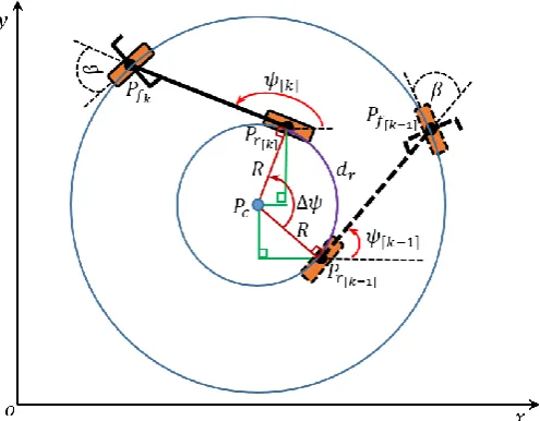
Fig. 2 illustrates the geometrical relationship between the bicycle’s previous position at time 𝑘 − 1 and its current position at time 𝑘.

It is assumed that between the two sample times the effective steering angle of the bicycle remains constant. So considering the frame yaw angle 𝜓 with reference to the x-axis at times 𝑘 −

1 and 𝑘, the instantaneous central angle Δ𝜓 in radians can be expressed as:

Δ𝜓 = 𝜓[κ]− 𝜓[κ−1] (3)

or as:

Δ𝜓 = 𝑑𝑟

𝑅 (4)

where 𝑑𝑟 is the length of the arc, which can also be

approximated as the ‘travelled distance’, from points 𝑃_𝑟𝑘−1to

𝑃_𝑟𝑘 in metres.

Equation (2) and (4) result into:

Δ𝜓 =𝑑𝑟∙ 𝑡𝑎𝑛(𝛽)

𝑊 (5)

A so called dead-reckoning (DR) algorithm can be developed in order to estimate the bicycle’s current position based upon a previously determined or known position [26]. The simplest form of the DR algorithm follows a two-step procedure where depending on the instantaneous turning angle, Δψ, the trajectory can be computed as follows:

(1) For an instantaneous turning angle 𝛽 of less than a certain tolerance angle, it can be simply approximated as a straight line:

𝑥[𝑘]= 𝑥[𝑘−1]+ 𝑑𝑟∙ 𝑐𝑜𝑠(𝜓[𝑘−1]) _(6a)

𝑦[𝑘]= 𝑦[𝑘−1]+ 𝑑𝑟∙ 𝑠𝑖𝑛(𝜓[𝑘−1])

(6b) (2) For an instantaneous turning angle of more than the

tolerance angle, the trajectory is an arc and can be approximated with a two-step method – firstly by computing the coordinates of 𝑃𝑐 and secondly by

updating the yaw angle as expressed below:

𝑃_{𝐶 𝑥}= 𝑥[𝑘−1]− 𝑅 ∙ 𝑠𝑖𝑛(𝜓[𝑘−1]) (7a)

𝑃_{𝐶 𝑦}= 𝑦[𝑘−1]+ 𝑅 ∙ 𝑐𝑜𝑠(𝜓[𝑘−1]) (7b)

𝜓[𝑘]= (𝜓[𝑘−1]+ 𝛥𝜓)𝑚𝑜𝑑2𝜋 (8)

𝑥[𝑘]= 𝑃_{𝐶 𝑥}+ 𝑅 ∙ 𝑠𝑖𝑛(𝜓[𝑘]) (9a)

𝑦[𝑘]= 𝑃_{𝐶 𝑦}− 𝑅 ∙ 𝑐𝑜𝑠(𝜓[𝑘]) (9b)

The above two-step DR procedure is not suitable as a predictor-corrector algorithm basically due to the presence of the “internal” variables 𝑃_{𝐶 𝑥} and 𝑃_{𝐶 𝑦} . Hence an alternative approximation positioning model is developed here.

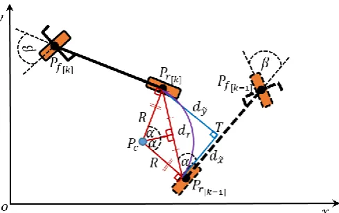
Based on the geometry of Fig. 2 and Fig. 3, the position of the rear frame between time 𝑡_𝑘−1 and 𝑡_𝑘 is given in body fixed coordinates by:

𝑑𝑥̃ = 𝑅𝑠𝑖𝑛(∆𝜓) (10a)

𝑑𝑦̃ = 𝑅 − 𝑅𝑐𝑜𝑠(∆𝜓) (10b)

Where the above two equations were simplified using the double-angle expressions for 𝑠𝑖𝑛(2𝛼) and 𝑐𝑜𝑠(2𝛼). Moreover, the parameters R and ∆𝜓 can be computed from (1), (2) and (5).

Fig. 3. Bicycle geometric relationship with body and global coordinates system

The kinematics model for the position of the bicycle in the global coordinate system is then portrayed by (11).

[𝑥_𝑦[𝑘]_[𝑘]]

= [𝑥_𝑦[𝑘−1]

[𝑘−1]]

+ [𝑐𝑜𝑠 (𝜓_{𝑠𝑖𝑛 (𝜓}[𝑘−1]) −𝑠𝑖𝑛(𝜓[𝑘−1])

[𝑘−1]) 𝑐𝑜𝑠 (𝜓[𝑘−1]) ] [

𝑑𝑥̃[𝑘−1]

𝑑𝑦̃[𝑘−1]]

(11)

where subscripts 𝑘 − 1 in 𝑑𝑥̃ and 𝑑𝑦̃ denote the computation of (10a) and (10b) between time 𝑘 − 1 and 𝑘.

Thus, the proposed model bypasses the estimation of the instantaneous centre of rotation of the two-step DR algorithm. Hence, the model can be readily used in the fusion algorithm as a position Kalman filter.

It should be noted that since the DR process depends on the accumulation of previous positions, calculated solely from bicycle’s data acquisition is prone to drift and is only suitable for a short time horizon. However, fusing this data with Global Navigation Satellite System (GNSS) and localisation systems based on ubiquitous wireless communications, widely found in urban areas, can lead to improved overall accuracy. Thus, the next section looks at the proposed fusion technique.

III. PROPOSED SENSOR FUSION TECHNIQUE

From the practical point of view, the Kalman filter algorithm is easy to implement and more suitable for real-time applications. Since the ultimate aim of the overall project is to integrate the developed algorithm in a real-time application, Kalman filter was chosen over other complex filters such as a Particle filter [27] and Bayesian filter [28].

A. Yaw Angle Kalman Filter

kinematic parameters, such as the roll angle which is considered with respect to earth (Fig. 1) can also be potentially noisy. One way to improve the accuracy is to employ multiple sensors to measure the same parameter with alternative approaches. To apply this method successfully, the data from the multiple sensors must be fused with an appropriate technique. For this reason, a Kalman filter algorithm is designed and the development of the mathematical models to fulfil the standard Kalman filter equations stated in the Appendix.

The relationship between the yaw angle (𝜓) and the yaw rate (𝜔 = 𝜓̇) at time scan 𝑘 and 𝑘 − 1 can be expressed as:

𝜓[𝑘]= 𝜓[𝑘−1]+ (𝜔[𝑘−1]∙ ∆𝑡) (12)

where ∆𝑡 is the time interval between two samples. From the above equation, the yaw rate can be then expressed as:

𝜔[𝑘−1]=

𝜓[𝑘]− 𝜓[𝑘−1]

∆𝑡 (13)

However, the measurement of the yaw rates using an electronic gyroscope also incorporates bias, 𝜔𝑏𝑖𝑎𝑠, as well as

measurement noise 𝑤_𝜔 [29]. Hence, at time instant 𝑘 − 1 the measured yaw rate can be expressed as:

𝜔[𝑘−1]= 𝜔𝑚[𝑘−1]− 𝜔𝑏𝑖𝑎𝑠[𝑘−1]− 𝑤𝜔[𝑘−1] (14)

where 𝜔𝑚[𝑘−1] is the measured yaw rate and acts as a known

input to the yaw model.

The yaw rate bias, which can be measured from experimental data, is normally considered to be unchanged, and therefore, the

𝜔𝑏𝑖𝑎𝑠 at time 𝑘 − 1 is:

𝜔𝑏𝑖𝑎𝑠[𝑘]= 𝜔𝑏𝑖𝑎𝑠[𝑘−1] (15)

Therefore, the yaw angle (𝜓) at time 𝑘 can be expressed as:

∴ 𝜓[𝑘]= 𝜓[𝑘−1]+ (𝜔𝑚[𝑘−1]− 𝜔𝑏𝑖𝑎𝑠[𝑘−1]

− 𝑤𝜔[𝑘−1]) ∙ ∆𝑡 (16)

Using 𝜓_[𝑘] and 𝜔_{𝑏𝑖𝑎𝑠[𝑘]} as states, and 𝜓_[𝑘] as an output and

𝜔𝑚[𝑘] as an input, (15) and (16) give rise to the following yaw

angle model:

𝑿[𝑘]= [_𝜔𝜓[𝑘]

𝑏𝑖𝑎𝑠[𝑘]] = [1 −∆𝑡0 1 ] [

𝜓[𝑘−1]

𝜔𝑏𝑖𝑎𝑠[𝑘−1]]

+ [∆𝑡

0] 𝜔𝑚[𝑘−1]+ 𝒘[𝑘−1]

(17a)

𝒁[𝑘−1]= [1 0] [_𝜔𝜓[𝑘]

𝑏𝑖𝑎𝑠[𝑘]] + 𝑣[𝑘−1] (17b)

Therefore, from the expressions above, the relevant parameters for the Kalman filter algorithm can be set as:

𝑿[𝑘]= [_𝜔𝜓[𝑘]

𝑏𝑖𝑎𝑠[𝑘]] , 𝒖[𝑘]= 𝜔𝑚[𝑘],

𝒁[𝑘]= 𝜓[𝑘]+ 𝑣[𝑘−1]

(18a)

𝑭 = [1 −∆𝑡

0 1 ] , 𝑩 = [∆𝑡0] , 𝑯 = [1 0] (18b)

Moreover, the covariance matrices 𝑸[𝑘] and 𝑹[𝑘] are

assumed constant of the following form:

𝑸[𝑘]= [𝜎𝜔 2 ₀

0 0] , 𝑅[𝑘]= 𝜎𝜓

2 ₍₁₉₎

where the values 𝜎_𝜔2 and 𝜎_𝜓2 can be approximated through a one-time experimental calibration using the well-known expression of variance of a random variable 𝛼̃ from 𝑁 observations:

𝜎𝛼̃2=

1

(𝑁 − 1)∑ |𝛼̃𝑖− 𝜇𝛼̃|2 𝑁

𝑖=1

(20a)

With

𝜇𝛼̃= _𝑁1∑ 𝛼̃𝑖 𝑁

𝑖=1

(20b)

B. Bicycle Position Kalman Filter

The position Kalman filter is based on the DR algorithm derived in Section II through (10a), (10b) and (11). Assuming the global position coordinates 𝑥[𝑘], 𝑦[𝑘] as states, and also as

outputs, and 𝑑𝑥̃[𝑘], 𝑑𝑦̃[𝑘] as inputs, equation (11) gives rise to

the following position model:

𝑿[𝑘]= [

𝑥[𝑘]

y[𝑘]]

= [1 0 0 1] [

𝑥[𝑘−1]

y[𝑘−1]]

+ [𝑐𝑜𝑠(𝜓[𝑘−1]) −𝑠𝑖𝑛 (𝜓[𝑘−1]) 𝑠𝑖𝑛 (𝜓[𝑘−1]) 𝑐𝑜𝑠(𝜓[𝑘−1])

] [𝑑𝑥̃_𝑑𝑦̃[𝑘−1]

[𝑘−1]]

+ 𝒘[𝑘−1]

(21a)

𝒁[𝑘−1]= 𝑿[𝑘−1]+ 𝒗[𝑘−1] (21b)

Where, 𝜓_[𝑘] is estimated from the Yaw Angle Kalman Filter stated in previous section.

Therefore, from the expressions above, the relevant parameters for the Kalman filter algorithms can be set as:

𝑿[𝑘]= [

𝑥[𝑘]

y[𝑘]] , 𝒖[𝑘]= [

𝑑𝑥̃[𝑘]

𝑑𝑦̃[𝑘]] , 𝒁[𝑘]= 𝑿[𝑘] (22a)

𝑭 = [1 0_{0 1}] , 𝑩[𝑘]= [𝑐𝑜𝑠(𝜓[𝑘]) − sin(𝜓[𝑘])

sin(𝜓[𝑘]) 𝑐𝑜𝑠(𝜓[𝑘])],

𝑯 = [1 0 0 1]

In addition, the covariance matrices 𝑸[𝑘] and 𝑹[𝑘] are

assumed again in this case constant of the following form:

𝑸[𝑘]= [

𝜎𝑠𝑦𝑠2 0

0 𝜎𝑠𝑦𝑠2 ] (23a)

𝑹[𝑘]= [

𝜎𝑝𝑜𝑠2 0

0 𝜎𝑝𝑜𝑠2 ]

(23b)

The value of 𝜎𝑠𝑦𝑠2 can be derived experimentally from the

filtered yaw angle and distance measurements, while the value of 𝜎_𝑝𝑜𝑠2 can be approximated experimentally from a number of observations of absolute measurements for a known location.

More information about accuracy and measurement rates of each sensor is beyond the scope of this paper and can be found in [30]. However, measurement noise, assumed to be of Gaussian distribution, was taken into account at present by one-time experimental calibration for the approximation of the covariance matrices in the implementation of the Kalman filters.

In summary, the four critical kinematics measurement parameters of steering angle (𝛿), roll angle (𝜙), yaw rate (𝜓̇ =

𝜔) and travelled distance (𝑑𝑟), along with two crucial bicycle

design parameters of wheelbase (𝑊) and caster angle (𝜂) are required to successfully implement the models. However, in general, sensor acquired data do not directly provide the required measurement parameters. This crucial part of data acquisition and processing in the case of the iBike is envisaged to be presented in a subsequent publication. A brief presentation of the implemented multi-sensor is provided in the following paragraphs;

• An absolute optical encoder is employed to measure the steering angle (δ) as this type of sensor maintains its position information even when the power is turned off and eliminates the need for a zero cycle.

• A Hall Effect gear-tooth speed sensor is used to measure the travelled distance (𝑑𝑟) of the rear wheel, where the

sensor detects small magnets mounted on the spokes.

• A 3-axis MEMS gyroscope is utilised to measure the yaw rate (𝜓̇) of the rear frame of the bicycle. The sensor’s roll rate is also exploited with a 3-axis MEMS accelerometer to compute the fused roll angle (𝜙) of the bicycle.

C. Design of the Overall Algorithms

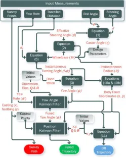
From the study of bicycle geometry and the derivation of the models in this paper, Fig. 4 illustrates the simplified design of the overall algorithms, together with the data flow. This design is utilised to transform bicycle motion measurements into relative positions and to fuse the positions with known control points discussed in the next section.

Overall, the algorithms take the input measurements data from the sensors and output a trajectory based on the DR technique described. The algorithms also produce a fused trajectory based on the Kalman filter models discussed in Sections III. A and III. B, where the known control points are randomly selected from survey points and for the purpose of testing and demonstrating the algorithm, the control points are

assumed as the positions based on Wireless Communication Technologies (WCT) and GNSS. Moreover, the random selection of the control points simulates the positions measurements from GNSS, as some measurements will be subject to a large position error and they cannot be fused with the sensor data. Finally, outputs also show the survey points as a path so that the DR and the fused trajectories can be compared.

Fig. 4. Design of the overall algorithms

IV. IMPLEMENTATION AND RESULTS

A. The iBike System Architecture

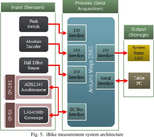
In order to implement the algorithms developed, a ‘Barclays Cycle Hire’ bicycle (now sponsored by Santander) has been supplied by Transport for London (TfL) and has been equipped with the MEMS gyroscope, MEMS accelerometer, and absolute encoder and Hall Effect sensors. The four of identified kinematics measurement parameters in Section III. B are continuously monitored and sampled at 66 Hz using these sensors. The measurements are then employed to determine the trajectory of the bicycle using the developed algorithms in the previous section.

the data in a relational database structure for future studies. The push switch is used as the controller for the data acquisition while a LED is used to indicate the status of the system.

Fig. 5. iBike measurement system architecture

Fig. 6 illustrates the actual instrumented bicycle with the sensor configuration. The frame sensor houses the accelerometer and gyroscope while the main control box incorporates the Arduino board along with various electronic components. In addition, a GoPro camera is also installed on the bicycle for the purpose of visual validation of the rear wheel path.

Fig. 6. The instrumented bicycle (iBike)

B. Field Experiment Setup and Results

Following the completion of the instrumentation of the bicycle, a route was selected around City University of London’s campus, as illustrated in Fig. 7 , and was then mapped using topographical surveying techniques, and specifically a Leica TCRA1103plus Total Station; this has a range of up to 2500 m and a distance measurement accuracy of 20 mm. The survey was conducted prior to the actual experiment with the iBike, and, as illustrated in Fig. 8, the precise coordinates of a number of points were measured and recorded using the UK Ordnance Survey (Eastings and Northings) coordinate system [31].

During the actual experiment, the instrumented bicycle was ridden directly over (or as close as possible to) the surveyed points. As a result, approximate coordinates of the bicycle at the surveyed locations were available and this enabled to

approximate the accuracy of the overall system with the proposed algorithms. The overall survey route consisted of 93 points and had an approximate length of 1050 m from start to end.

Fig. 7. Satellite view of the experimental route

The results obtained from a single journey along the surveyed route are illustrated in Fig. 9, where the blue line represents the computed path from the iBike sensor data and the DR model and the green line represents the fused trajectory based on the Kalman filters. The red hollow circles represent the survey points established prior to the experiment, while the solid black dots represent the control points used for the bicycle position Kalman filter, discussed in Section III. B. Finally, the red star denotes the initial position used in the algorithm illustrated in Fig. 4.

As can be seen from the graph, the reconstructed trajectory based on the iBike data with the DR technique alone is prone to drift; however, the fused trajectory, based on the Kalman filters and a random selection of control points from the survey, clearly indicates an improvement on the overall results. Consequently, this demonstrates that the sensor fusion algorithm applied in this study improves significantly the positioning accuracy. As a result, the overall methodology can be applied to accurately track cyclists and it can potentially be utilised with a collision warning algorithm to minimise the occurrence of false alerts.

Furthermore, to examine the accuracy of the overall methodology, a k-nearest neighbours algorithm, available through MATLAB’s “knnsearch” function, was applied to the generated trajectories together the survey points. This process aided to extract the points which are correlated with the survey

points and allowed to compute the error at each survey point for the DR and fused trajectories.

Fig. 9. Comparison of the trajectories

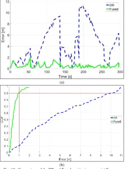
Fig. 10 presents error versus time and the comparison of the Cumulative Distribution Function (CDF) of the positioning error between the survey points and computed trajectories based on the DR and fused algorithms.

(a)

(b)

Fig. 10. Comparison of the DR and Fused positioning error: (a) Error vs. Time and (b) CDF vs. Error

It is clear from the above graph that the sensor fusion technique proposed in this paper enhances the results; in fact,

with 90% probability a position can be estimated with an accuracy of 1 m or less. On the other hand, the DR error accumulates, and it can be used to estimate a position with an accuracy of 1 m or less only with a 10% probability.

It should be additionally noted here that, due to practical reasons pertaining to the cyclist’s vision and skill, as well as to the surrounding traffic conditions, the bike could often not be ridden exactly over the survey points. This meant that there was very likely an inherent error in the measurement relating purely to external factors rather than to the system itself. Thus, the actual positioning error could be even lower than what is reported in this study.

V. CONCLUSIONS AND FUTURE WORK

From the analysis of its unique characteristics, it can be easily understood that a bicycle is an “underactuated” system, in that it has fewer control variables than degrees of freedom. However, under normal conditions a bicycle’s motion is controlled through three essential parameters: steering angle, tilt angle and speed. Thus, the kinematics and the turning geometry of a bicycle were studied here to formulate a geometric relationship of the steering mechanism. Then a simplified model was developed for a dead-reckoning algorithm, enhanced through two sets of Kalman filter models to correct for the yaw angle and position errors over time in order to prevent drifting errors over long distances. The multi-sensor fusion algorithm was then successfully applied to field data collected using the developed iBike system and the known chosen coordinates (control points) from the survey path. The overall results of the field experiments show that it is possible to achieve a higher position accuracy using the developed algorithms.

Although the field experiment was successful in a typical urban environment, the authors would like to point out that weather condition and environmental features such as tall buildings, trees and reflecting surfaces could pose limitations on the proposed technique when especially GNSS is used for the correction part of the algorithm. However, the error could be minimised by using other existing technologies such as Wi-Fi and mobile base stations, alongside GNSS.

As such, the future work on bicycle accurate positioning will concentrate on the collection of measurements from Wireless Communication Technologies (WCT), which are widely available in urban areas, as well as GNSS and use these data in an improved sensor fusion algorithm. The problem of robustness could also be addressed within this framework.

Finally, the authors believe that the improved sensor fusion algorithm could constitute a credible basis for the development of future collision warning and avoidance systems.

APPENDIX

which is theoretically more suitable for the fusion of noisy sensor data. The algorithm works in a two-stage process: (1) it produces estimations of the current state variables along with their uncertainties; (2) then it updates the estimations by utilising a weighted average. The two-stage process of the discrete Kalman filter described in [32] and [33] is based on a linear time varying state space representation as followings:

𝑿[𝑘]= 𝑭[𝑘−1]𝑿[𝑘−1]+ 𝑩[𝑘−1]𝒖[𝑘−1]+ 𝒘[𝑘−1] (24a)

𝒁[𝑘−1]= 𝑯[𝑘−1]𝑿[𝑘−1]+ 𝒗[𝑘−1] (24b)

where 𝑿[𝑘] is the state vector at time 𝑘, 𝑭[𝑘] is the state

transition matrix at time 𝑘, 𝑩[𝑘] is the control input matrix, 𝒖[𝑘]

is the vector containing any control inputs, 𝒘_[𝑘] is the Gaussian process noise with covariance matrix 𝑹_[𝑘], 𝒁[𝑘] is the vector of

measurements, 𝑯[𝑘] is the output matrix and 𝒗[𝑘] is the

Gaussian measurement noise with covariance matrix 𝑸_[𝑘]. For the estimation of states at time 𝑘, the Kalman filter algorithm is performed by two steps, known as “prediction” and “update”, and they are described mathematically below:

1. Prediction:

𝑿̂[𝑘|𝑘−1]= 𝑭[𝑘−1]𝑿̂[𝑘−1|𝑘−1]+ 𝑩[𝑘−1]𝒖[𝑘−1] (25a)

𝑷[𝑘|𝑘−1]= 𝑭[𝑘−1]𝑷[𝑘−1|𝑘−1]𝑭[𝑘−1]𝑻 + 𝑸[𝑘−1] (25b)

2. Update:

𝑲[𝑘]= 𝑷[𝑘|𝑘−1]𝑯[𝑘−1]𝑻 (𝑯[𝑘−1]𝑷[𝑘|𝑘−1]𝑯[𝑘−1]𝑻

+ 𝑹[𝑘−1])

−𝟏 (26a)

𝑿̂[𝑘|𝑘]= 𝑿̂[𝑘|𝑘−1]+ 𝑲[𝑘](𝒁[𝑘]− 𝑯[𝑘]𝑿̂[𝑘|𝑘−1]) (26b)

𝑷[𝑘|𝑘]= 𝑷[𝑘|𝑘−1]− 𝑲[𝑘]𝑯[𝑘]𝑷[𝑘|𝑘−1] (26c)

where 𝑲_[𝑘] is the optimal Kalman gain, 𝑷_{[𝑘|𝑘−1]} is the covariance matrix (confidence) before data fusion, 𝑷[𝑘|𝑘] is the

covariance matrix (confidence) following data fusion, 𝑿̂[𝑘|𝑘−1]

is the state vector before data fusion, and 𝑿̂[𝑘|𝑘] is the state

vector following data fusion.

ACKNOWLEDGMENT

The authors would like to thank Transport for London for supplying the Santander Cycle Hire bicycle used in this study.

REFERENCES

[1] TfL, “Cycling,” [Online]. Available: https://tfl.gov.uk/modes/cycling/. [Accessed 25 July 2017].

[2] A. Nikitas, P. Wallgren and O. Rexfelt, “The paradox of public acceptance of bike sharing in Gothenburg,” Proceedings of the Institution of Civil Engineers - Engineering Sustainability, vol. 169, no. 3, pp. 101 - 113, 2016.

[3] D. Horton, P. Rosen and P. Cox, “Fear of Cycling,” in Cycling and Society, Hampshire, Ashgate, 2012, pp. 133-151.

[4] A. Thornton, L. Evans, K. Bunt, A. Simon, S. King and T. Webster , “Climate Change and Transport Choices,” TNS BMRB, London, 2011.

[5] RoSPA, “Road Safety Factsheet - Cycling Accidents,” July 2017. [Online]. Available: https://www.rospa.com/rospaweb/docs/advice-services/road-safety/cyclists/cycling-accidents-factsheet.pdf. [Accessed 31 July 2017].

[6] DfT, “Reported Road Casualties in Great Britain: Quarterly Provisional Estimates Q2 2015,” 5 November 2015. [Online]. Available:

https://www.gov.uk/government/uploads/system/uploads/attachment_ data/file/473850/quarterly-estimates-april-to-june-2015.pdf. [Accessed 5 November 2015].

[7] DfT, “Reported road casualties in Great Britain: main results 2015,” National Statistics, 30 June 2016. [Online]. Available:

https://www.gov.uk/government/uploads/system/uploads/attachment_ data/file/533293/rrcgb-main-results-2015.pdf. [Accessed 03 May 2017].

[8] European Commission, “Traffic Safety Basic Facts 2017 – Cyclists,” European Commission, Directorate General for Transport, Brussels, 2017.

[9] National Center for Statistics and Analysis, “Bicyclists and Other Cyclists: 2015 data,” National Highway Traffic Safety Administration, Washington, DC, 2016.

[10] F. Kuster, C. Laurence and R. Geffen, “Halving injury and fatality rates for cyclists by 2020,” ECF , Brussels, 2010.

[11] S. Schoon, M. Doumen and D. de Bruin, “The circumstances of blind spot crashes and short- and long-term measures,” SWOV report no. R-2008-11A & B, 2008.

[12] TfL, “Blaze Laserlights,” [Online]. Available:

https://tfl.gov.uk/modes/cycling/santander-cycles/blaze-laserlights. [Accessed 25 July 2017].

[13] Volvo, “Collision warning – Cyclist detection,” 2016. [Online]. Available: http://support.volvocars.com/en-CA/cars/Pages/owners-manual.aspx?mc=y286&my=2016&sw=15w17&article=3bf022eeedf 3242bc0a801e80043a9f6. [Accessed 25 July 2017].

[14] G. French, J. Steer and N. Richardson, “Handbook for cycle-friendly design,” Sustrans, 11 April 2014. [Online]. Available:

http://www.sustrans.org.uk/sites/default/files/file_content_type/sustran s_handbook_for_cycle-friendly_design_11_04_14.pdf. [Accessed 2 May 2017].

[15] H. Lyu, L. Kong, C. Li, Y. Liu, J. Zhang and G. Chen, “BikeLoc: a Real-time High-Precision Bicycle Localization System Using Synthetic Aperture Radar,” in Proceedings of the First Asia-Pacific Workshop on networking, Hong Kong , 2017.

[16] S. Stasinopoulos, M. Zhao and Y. Zhong, “Simultaneous localization and mapping for autonomous bicycles,” International Journal of Advanced Robotic Systems, vol. 14, no. 3, p. 1–16, 2017.

[17] U-blox, “3D Automotive Dead Reckoning chip: a new dimension in navigation,” 2017. [Online]. Available: https://www.u-blox.com/en/u-blox-3d-automotive-dead-reckoning-technology. [Accessed 15 June 2017].

[18] Advanced Navigation, “SPATIAL,” 2015. [Online]. Available: https://www.advancednavigation.com.au/product/spatial. [Accessed 15 June 2017].

[19] S. F. Campbell, “Steering control of an autonomous ground vehicle with application to the DARPA urban,” 2007.

[20] T. D. Gillespie, Fundamentals of Vehicle Dynamics, Society of Automotive Engineers, 1992.

[21] A. De Luca and G. Oriolo, “FEEDBACK CONTROL OF A NONHOLONOMIC CAR-LIKE ROBOT,” Rome, 2004. [22] V. Cossalter, Motorcycle Dynamics, 2nd English Edition ed., Lulu,

2006.

[24] G. Franke, W. Suhr and F. Riel3, “An advanced model of bicycle dynamics,” European Journal of Physics, vol. 11, pp. 116-121, 1990. [25] J. Yi, D. Song, A. Levandowski and S. Jayasuriya, “Trajectory

tracking and balance stabilization control of autonomous motorcycles,” Robotics and Automation, pp. 2583-2589, 2006. [26] S. Miah, I. Kaparias, D. M. Stirling and P. Liatsis, “Development and

Testing of a Prototype Instrumented Bicycle For The Prevention of Cyclist Accidents,” in Transportation Research Board (TRB) 95th Annual Meeting, Washington D.C., USA, 2016.

[27] T. Yang, P. G. Mehta and S. Meyn, “Feedback Particle Filter,” IEEE Transactions on Automatic Control, vol. 58, no. 10, pp. 2465-2480, 2013.

[28] S. Zhang, S. C. Chan, B. Liao and K. M. Tsui, “A New Visual Object Tracking Algorithm Using Bayesian Kalman Filter,” in IEEE International Symposium on Circuits and Systems (ISCAS), Melbourne, 2014.

[29] P. Wang and C.-Y. Chan, “Vehicle Collision Prediction at Intersections based on Comparison of Minimal Distance Between Vehicles and Dynamic Thresholds,” IET Intelligent Transport Systems, vol. 11, no. 10, 2017.

[30] S. Miah, I. Kaparias and P. Liatsis, “Evaluation of MEMS sensors accuracy for bicycle tracking and positioning,” in International Conference on Systems, Signals and Image Processing (IWSSIP), London, 2015.

[31] Ordnance Survey, “A guide to coordinate systems in Great Britain,” Britain’s mapping agency, Southampton, 2016.

[32] F. Ramsey, “Understanding the Basis of the Kalman Filter Via a Simple and Intuitive Derivation [Lecture Notes],” IEEE Signal Processing Magazine, vol. 29, no. 5, pp. 128-132, 2012.

[33] K. Ogata, Discrete-time Control Systems, New Jersey: Prentice Hall, 1995.

Shahjahan Miah graduated with a

first-class honours MEng degree in Electrical and Electronic Engineering from City, University of London, UK, in 2012. He has recently completed his PhD in systems and modelling with a focus on transport applications from the same institution. Alongside his PhD, he has also worked as a Research Assistant on a number of collaborative projects at the Research Centre for Systems and Control, and has also undertaken independent teaching activities on modules of City University’s undergraduate Mechanical and Electrical Engineering programmes. He has also served as a Reviewer for the IET Intelligent Transport Systems and Part C: Journal of Mechanical Engineering Science. His research interests are in the area of intelligent transport systems and robotics.

Efstathios Milonidis received his first degree in Electrical Engineering from the National Technical University of Athens in 1981, his MSc in Control Engineering and his MPhil in Aerodynamics and Flight Mechanics from Cranfield Institute of Technology in 1984 and 1986 respectively. He then received a PhD in Control Theory and Design from City, University of London in 1994.

He is currently a Senior Lecturer in Control and Information Systems and a Director of UG Studies in the Dept. EEE, City, University of London, UK. His research interests are in the area of discrete-time control, mathematical modelling and simulation of dynamical system and flight mechanics.

Ioannis Kaparias graduated with a

Master of Engineering (MEng) degree in Civil Engineering from Imperial College London in 2004. He then joined the Centre for Transport Studies of Imperial for his PhD research on the topic of “Reliable Dynamic In-vehicle Navigation”, which he completed in 2008, and continued as a post-doctoral Research Associate in the same institution for a period of four years, working on a wide range of transport research projects. From 2012 he held a Lecturer position at City University of London and in 2016 he joined the Transportation Research Group of the University of Southampton as a Lecturer in Transport Engineering. His research interests include traffic engineering, modelling and simulation, Intelligent Transport Systems, network reliability, travel demand, travel behaviour, and public realm, and his work has led to several journal publications and presentations at international conferences.

Nicholas Karcanias received the

Diploma in Mechanical and Electrical Engineering, with specialisation in Electrical, from the National Technical University of Athens in 1972 and the M.Sc and Ph.D degrees in Control Engineering from UMIST, England in 1973 and 1976 respectively. He received his DSc from City, University of London, UK in 1990 for his contributions to Control Theory.