Retrospective Theses and Dissertations Iowa State University Capstones, Theses and Dissertations
1-1-1993
A scanning electron microscope study of rat sciatic
nerve fiber regeneration through silicone rubber
single lumen nerve cuffs
Yueh-Sheng Yueh-Sheng
Iowa State University
Follow this and additional works at:https://lib.dr.iastate.edu/rtd Part of theEngineering Commons
This Thesis is brought to you for free and open access by the Iowa State University Capstones, Theses and Dissertations at Iowa State University Digital Repository. It has been accepted for inclusion in Retrospective Theses and Dissertations by an authorized administrator of Iowa State University Digital Repository. For more information, please [email protected].
Recommended Citation
Yueh-Sheng, Yueh-Sheng, "A scanning electron microscope study of rat sciatic nerve fiber regeneration through silicone rubber single lumen nerve cuffs" (1993).Retrospective Theses and Dissertations. 18014.
A scanning electron microscope study of rat sciatic nerve fiber regeneration through silicone rubber single lumen nerve cuffs
by
Yueh-Sheng Chen
A Thesis Submitted to the
Graduate Faculty in Partial Fulfillment of the Requirements for the Degree of
MASTER OF SCIENCE
Interdepartmental Program: Biomedical Engineering Major: Biomedical Engineering
Signatures have been redacted for privacy
Iowa State University Ames, Iowa
ii
TABLE OF CONTENTS
1. INTRODUCTION
2. LITERATURE REVIEW
2.1. Background
2.1.1. The mammalian peripheral nervous system 2.1 .2. Nerve degeneration
2.1.3. Nerve regeneration 2.2. Repair techniques
2.3. Characteristics of the silicone rubber cuffs 2.4. Silver staining of nerve tissue
2.5. Scanning electron microscopy 2.5.1 . Secondary electrons 2.5.2. Backscatter electrons
3. MATERIALS AND METHODS
3.1. Samples
3.2. Light microscopy and scanning electron microscopy 3.3. Quantitative evaluations
3.3.1. Quantitative studies
3.3.2. Preparation of fiber diameter histograms 3.4. Statistical methods
4. RESULTS
4.1. Microstructure 4.1 .1. Control
4.1.2. Proximal section
4.1.3. Middle section 4.1.4. Distal section 4.2. Fiber diameter histograms
iii
4.2.1. Fiber diameter histograms observed using LM 4.2.2. Fiber diameter histograms observed using SEM 4.3. Quantitative results
4.3.1. Quantitative results from LM 4.3.2. Quantitative results from SEM
5. DISCUSSION
6. CONCLUSIONS
BIBLIOGRAPHY
ACKNOWLEDGEMENTS
APPENDIX: FIBER DIAMETER HISTOGRAMS
29
iv
LIST OF FIGURES
Figure 2.1: Schematic representation of the structure of a mammalian
peripheral nerve 5
Figure 4.1: Secondary electron micrograph of a cross-section of the right sciatic nerve at the mid-thigh level from a normal control,
(animal #9, 24 weeks). Bodian stain. Scale bar=10 µm 25 Figure 4.2: Backscatter electron micrograph of the identical field as
Figure 4.1. Axons are the bright features surrounded by myelin sheaths. Bodian stain . Scale bar=10 µm 25 Figure 4.3: Backscatter electron image of a single-lumen cuff repaired nerve
section, (animal #48, middle section, 24 weeks). Category I and category II axons are in the field of view. Bodian stain. Scale bar
=10 µm 27
Figure 4.4: Backscatter electron image showing silver grains on the surface for a region of a single-lumen cuff nerve section, (animal #41, middle section, 24 weeks). Some regions of nerve sections were heavily covered with these features whereas even on the same section there were regions with relatively few particles of this
type on the surface. Bodian stain. Scale bar=2 µm 27 Figure 4.5: Backscatter electron image of a single-lumen cuff nerve section,
(animal #6, proximal section, 24 weeks). Microfascicles are apparent. Category I and category II axons are seen. Bodian
stain. Scale bar=10 µm 30
Figure 4.6: Backscatter electron image of a single-lumen cuff nerve section, (animal #6, middle section, 24 weeks) . Category I and category II axons are seen. Bodian stain. Scale bar=10 µm 30
v
LIST OF TABLES
Table 3.1: Implant period, type of repair, animal number, nerve section, and slide number for sections used in the present LM and SEM
study 20
Table 4.1: Distributions of percentage of axons within ±1 µm of the mean
diameter observed using LM 35 Table 4.2: Distributions of percentage of category I axons within ±1 µm of
the mean diameter observed using SEM 36 Table 4.3: Distributions of percentage of category II axons within ±1 µm of
the mean diameter observed using SEM 37 Table 4.4: Distributions of percentage of total axons within ±1 µm of the
mean diameter observed using SEM 38 Table 4.5: Axon counts, reference area and axons per unit area observed
using LM 44
Table 4.6: Category I axon counts, reference area and category I axons
per unit area observed using SEM 45
Table 4.7: Category II axon counts, reference area and category II axons
per unit area observed using SEM 46 Table 4.8: Total axon counts, reference area and axons per unit area
observed using SEM 47
Table 4.9: Mean axon diameter, nerve area and percentage of nerve
observed using LM 48
Table 4.10: Mean category I axon diameter, nerve area and percentage
of nerve observed using SEM 49 Table 4.11 : Mean category II axon diameter, nerve area and percentage
of nerve observed using SEM 50 Table 4.12: Mean total axon diameter, nerve area and percentage of
nerve observed using SEM 51 Table 4.13: Diameter ratio and estimated total axons in each nerve
vi
Table 4.14: Category I axon diameter ratio and estimated total category I
axons in each nerve cross section observed using SEM 53 Table 4.15: Category II axon diameter ratio and estimated total category II
axons in each nerve cross section observed using SEM 54 Table 4.16: Axon diameter ratio and estimated total axons in each nerve
cross section observed using SEM 55 Table 4.17: Mean axon diameter comparisons between repaired nerve
sections and normal control observed using LM 57
Table 4.18: Mean axon diameter comparisons between nerve sections in
the same animal observed using LM 58 Table 4.19: Mean diameter comparisons of the same category of axons in
repaired nerve sections and in normal control observed using
SEM 59
Table 4.20: Mean axon diameter comparisons between repaired nerve
sections and normal control observed using SEM 61 Table 4.21 : Diameter comparisons between the category I and the category
II axons in the same nerve section observed using SEM 62 Table 4.22: Mean diameter comparisons of the same category of axons in
different nerve sections observed using SEM 63 Table 4.23: Mean diameter of total axons comparisons between nerve
sections in the same animal observed using SEM 65
Table 4.24: Diameter comparisons of axons in the same nerve section
1
1. INTRODUCTION
A number of techniques have been developed to repair damaged or dissected peripheral nerves. They include end-to-end suturing, fascicular suturing, nerve grafts, and nerve bridges. The choice of techniques depends upon the clinical situation and the surgeon's preference.
The end-to-end and the fascicular suture repair techniques are suitable for the nerve defect or injury which does not extend more than several millimeters. However, both of the techniques have their own disadvantages. In the end-to~end suturing technique, even though the outermost (epineural) layer of the dissected nerve ends is sutured together, poor alignment of fascicles and ingrowth of scar tissue into the nerve junction will result in unsatisfactory nerve function recovery (Marshall et al., 1989). In the fascicular suturing technique, a more precise alignment of fascicles is expected; however, the increased trauma to the perineurial and the intrafascicular tissue caused by the sutures will retard the nerve regeneration.
2
nerve described by Daniel (1991) was the first attempt to develop a lumen nerve cuff to bridge a gap for peripheral nerve repair. The multiple-lumen repair cuff provides orientation, mechanical support, and guidance for the outgrowing Schwann cells and regenerating axons.
3
4
2. LITERATURE REVIEW
2.1 Background
2.1.1 The mammalian peripheral nervous system
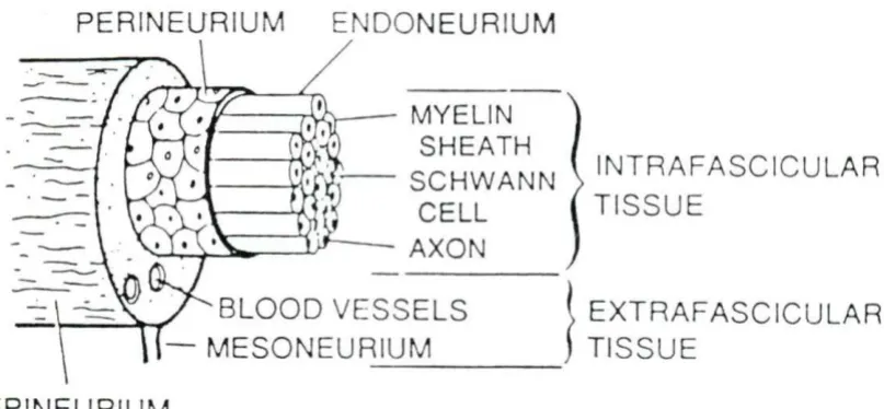
Peripheral nerves are composed of numerous nerve fibers collected into several fascicles (bundles) and covered with a connective tissue sheath, the epineurium. Each fascicle within the epineurium is surrounded by a perineurium consisting of an outer connective tissue layer and an inner layer of flattened epithelioid cells. Each nerve fiber and associated Schwann cell has its own slender connective tissue sheath , the endoneurium. The endoneurium components include fibroblasts, an occasional macrophage, and collagenous and reticular fibers.
Each axon can be classified as myelinated or unmyelinated, depending on whether or not it has a coating of myelin. The region of the exposed axon at the junction between Schwann cells is called the node of Ranvier. These nodes are located at discrete intervals along the whole length of the myelinated axon (Jenq et al., 1986). Figure 2.1 is a schematic representation of a mammalian peripheral nerve and its components (Marshall et al., 1989).
2.1.2 Nerve degeneration
5
PERINEURIUM ENDONEURIUM
. - -: .
·
--v----r'-1:'..-- MY ELIN
SHEATH
- SCHWANN
CELL AXON
INTRA FASCICU LAR TISSU E
----r
BLOOD VESSELS } EXTRAFASCICULAR [image:12.572.82.486.124.311.2]- MESONEURIUM
- ---
TI SSUE EPINEURIUMFigure 2.1: Schematic representation of the structure of a mammalian peripheral nerve (Marshall et al., 1989)
Regeneration begins from the undegenerated proximal stump. It remains connected to the trophic center. Many factors such as the site of the lesion, the age of the individual, the length of the nerve destroyed, the width of the severance gap, the alignment of the cut ends, and the amount of damage and hemorrhage in adjacent tissues affect the growth and development of the regenerating nerve (Swaim, 1987).
6
7
shrink or disappear. If regenerating axons do not invade into the distal nerve stump, the distal stump becomes even more contracted and is replaced by connective tissue (Swaim, 1987).
Many investigators (O'Daly and lmaeda, 1967; Calabretta et al. , 1973; Gershenbaum and Rosen, 1978; Ide et al., 1983; Tohyama et al., 1986) have observed the morphological alterations in the nerve fibers and connective tissues associated with Wallerian degeneration using light, transmission, and scanning electron microscopy. These studies provide a detailed account of the changes which occur during the degeneration of myelinated axons.
2.1.3. Nerve regeneration
8
The enlargement of the neuronal soma may peak early in the regeneration process and again as myoneural junctions are formed. The cell body may die if the injury is too close to it or, if it survives, the cell may not have enough metabolic capacity to support the axons that must be regenerated and axonal regeneration will not happen.
New protoplasm that is synthesized by the cell body migrates by axoplasmic flow from the neuronal soma down the axon. The axoplasmic flow has a slow and a fast component. The slow component (1 mm/day) involves microperistalsis within the nerve trunk membrane, and the fast component (1 OOmm/day) involves the microtubules. During the passage down the axon, a part of slowly transported proteins is used to replace catabolized enzymes in the membrane. Nevertheless, most of the proteins still reach the terminal segments of the axon. Microtubules provide the fast transport of axoplasm to supply the increased nutrient requirements and
metabolic activity at the synaptic regions.
The changes that occur at and between the proximal and distal nerve stumps strongly influence the regeneration of a severed nerve. Proliferation of epineurial and endoneurial connective tissue, Schwann cells, and capillaries, which control the regeneration of axons at the proximal and distal nerve stumps occur within 1 to 3 days after injury. These tissues infiltrate the injury site and migrate toward each other and form a bridge and capillary bed between the stumps to make it easier for the regenerating axons to grow to the distal nerve stump.
9
Different types of injury result in different locations for the start of sprouting or budding of the regenerating axons. Budding begins at 1 to 3 cm proximal to the point of severance in the case of wide-spread traumatic injuries; however, this budding begins a few millimeters retrograde to the last node of
Ranvier with a sharply localized injury.
Schwann cells of the proximal and distal nerve stumps probably play the most important role in axonal regeneration. As Schwann cells proliferate, they form longitudinally oriented bands of Bungner, which are continuous with the persisting Schwann tubes in the nerve stump (Allt, 1976; Spencer, 1977). The Schwann cells of each stump migrate toward each other and join. Because the Schwann cells of the proximal stump slightly precede those of the distal stump, they can be regarded as a guide for the regenerating axons. The rate of axonal regeneration at the marginal zone of realignment progresses about 0.25 mm/day. Beyond this point, regeneration occurs at the rate of 1 to 4 mm/day. Although 3 to 4 mm/day rate of regeneration for axonal tips occurs, the rate of functional return is only 1 to 2 mm/day. The axonal regeneration rate changes during the course of regeneration in a single nerve, with lag periods at the beginning and end of regeneration. The state of the motor end plate and the condition of health of the muscle fibers also influence the success of axonal regeneration. Thus, physical therapy and care of muscles and skin are important for successful peripheral nerve regeneration (Swaim , 1987).
10
of blood vessel, perineurial and epineurial tissue and a decrease in the amount of neural elements. In addition, dramatic increases in fibrous tissue and an absence of normal fascicular patterns were seen in the regenerated nerves (Mathur et al., 1983; Gibson and Daniloff, 1989). A smaller mean axon diameter and a larger number of regenerated axons in the repaired nerves as compared to the normal control were also reported (Rosen et al., 1983, 1989; Henry et al., 1985).
2.2. Repair techniques
Different types of injury and the gap length require different methods of nerve repair. For gap lengths less than 1 O mm, the end-to-end anatomosis is optimal. However, for gap lengths larger than 1 O mm, a graft is preferred. The autograft is the best option to repair injury nerves because it will not cause severe tissue reaction during the implantation period. Nevertheless, disadvantages of the autograft are the difficulty of acquiring a donor nerve for grafting and the inevitable risks of surgery at another site. To solve these problems, artificial nerve cuffs or guide tubes have been regarded as an alternative in the repair of injured nerves. Compared with nerve grafting , the implantation of nerve cuffs has resulted in good nerve regeneration.
Previous work in developing the artificial nerve cuffs and the materials used to fabricate them is described below.
11
polyglycolic acid conduit and the regrowth of myelinated axons grouped into "mini-fascicles" containing increased connective tissue.
Seckel et al. (1984) used biodegradable nerve guides made of DL-lactic acid (internal diameter=2 mm, wall thickness=250 µm) to bridge 5 mm and 10 mm gaps in adult Sprague-Dawley rats. Three months after repair, they observed the sciatic nerve of the adult rat successfully regenerated across the 5 mm gap through the biodegradable nerve guides, but across the 10 mm gap. They also found nerve regeneration in the biodegradable nerve guides did not elicit an evident immune response.
Satou et al. (1986) used a silicone tube filled with a small amount of collagen gel (Cell Matrix II) to study axon regeneration across a 5 mm gap in the rat sciatic nerve and compared it with the control side in which the gap space in the tube was left empty. They found more rapid growth of sprouting axons toward the distal stump in the collagen gel filled tube as compared to the control side. In addition, the proliferation of both fibroblasts and larger Schwann cells was inhibited. They concluded that appropriate exogenous fine material such as a collagen matrix can accelerate the regeneration of nerves in the silicone tube.
12
In 1989, Gibson and Daniloff used a silicone tube (Silastic, Dow Corning, 8mm in length) to bridge a gap of 5 mm in adult female Sprague-Dawley rats and compared it with a nerve allograft. Electromyography was used to provide an objective assessment of functional nerve regeneration. At 90 days post-implantation, the nerve graft group had superior conduction velocity times as compared to the silicone implant group. They suggested that if a nerve cuff is used in repair of a transected nerve, it should be large enough to accommodate nerve enlargement or should be removed after the regenerating axons have bridged the transection site.
In 1992, Rosen et al. used a synthetic biodegradable conduit made of glycolide trim ethylene carbonate (10 mm long) filled with a liquid collagen (Collagen {C3511]) to bridge gaps of 5 mm in adult Sprague-Dawley rat peroneal nerves. They compared the results for this case with sutured autografts. These rats were evaluated after 6 to 9 months of repair. They observed that there is negligible inflammatory response to the collagen matrix. Regenerated axon diameters were equal in the synthetic biodegradable conduit groups as compared to the sutured autograft groups.
2.3. Characteristics of the silicone rubber cuffs
13
Cross-linking (vulcanization) is the process by which the polymer is turned into the three dimensional structure of a rubber with all its associated properties (Van Noort and Black, 1981 ). This process is initiated by a catalyst which in the case of heat vulcanizing silicone rubber is a dichlorobenzoyl peroxide (DBP). DBP will break down to form free radicals and release carbon dioxide while heated over 60° C.
The dichlorophenyl radicals which have the properties of strong dehydration and oxidization can activate the methyl and vinyl chains by a radical transfer mechanism. Cross links then can be established by these activated vinyl and methyl groups. This reaction can take place in many ways. In general, methyl-methyl and methyl-vinyl interactions are the two most commonly used (Braley, 1970).
2.4. Silver staining of nerve tissue
14
Even though the exact reactions responsible for the selective affinity of Bodian's stain for neurofilament proteins remain to be discovered, the details of the chemical reactions that occur during the silver staining are well known.
In the early stage of the staining, impregnation by silver results in the formation of silver nuclei in both axons and myelin. However, after exposure of the section to the action of reducing agents (e.g. formalin , pyrogallol, or hydroquinone) , the impregnation of axons increases without the myelin being affected. The phenomena can be explained by assuming that the axons contain more reducing groups than myelin (Wolman, 1955). After sections are impregnated by silver solutions, the sections can be treated with gold chloride to intensify the contrast between the more strongly stained areas and the less intensely impregnated sites.
2.5. Scanning electron microscopy
SEM provides three-dimensional information which can aid in the interpretation of the two-dimensional ultrastructural changes seen with the light or the transmission electron microscope (Gershenbaum and Roisen , 1978). The powerful capability of the scanning electron microscope for the study of nerve tissue is due to the interactions between the primary beam electrons and the specimen atoms. These interactions may be placed into two groups:
15
loss. These kinds of scattered electrons are referred to as backscatter electrons.
(2) . Inelastic collisions. A primary beam electron collides with a specimen atom and results in a loss of energy from that atom, leading to the generation of secondary electrons, Auger electrons, characteristic and continuum X-rays.
The electrons are collected by a detector system (a different system for each variety) and converted to an electronic signal which is displayed on a cathode ray tube. The scanning of the SEM beam is synchronized with the scanning of the electron beam of the cathode ray tube, thus producing a representation of the area scanned on the CRT. Secondary electrons and/or backscatter electrons are frequently used in providing nerve tissue microstructural information.
2.5.1. Secondary electrons
The low energy electrons emitted from a sample with an energy less than 50 eV are usually regarded as the secondary electrons. The escape depth of secondary electrons represents only a small fraction of the primary electron range. The secondary emission images provide information about the surface topography.
2.5.2. Backscatter electrons
16
17
3. MATERIALS AND METHODS
3.1 Samples
A new type of nerve repair cuff, the multiple-lumen silfcone rubber nerve cuff, was described by Daniel ( 1991). Observations made from the multiple-lumen cuff nerve repairs were compared with results obtained from normal controls, end-to-end nerve repairs, and single-lumen silicone rubber cuff repairs. Sixteen Sprague-Dawley adult male rats were used by Daniel for single-lumen silicone rubber cuff studies. The current project is an extension of these studies with an emphasis on single lumen nerve cuff repair. These nerve specimens had been sectioned at 1.5 to 2.5 µm thick, silver stained, toned with gold chloride, and mounted on microscopic slides for light microscopic observations. The slides were obtained from proximal, middle, and distal sciatic nerve sections obtained at 8, 12, 16, and 24 weeks after implantation.
18
3.2 Light microscopy and scanning electron microscopy
Micrographs of a normal control and the proximal, middle, and distal cross-sections of the regenerated nerves from the single lumen silicone rubber cuff studies were taken by light and scanning electron microscopy. The light micrographs were taken at 160X with a Dialux 20 (Leitz) light microscope. The type of film used was TP135-36 Kodak Technical Pan film.
19
voltage of 15 kV, an aperture size of 70 µm, and a probe current of 0.02 to 0.3 nA. In addition, a smaller working distance (7 mm or 13 mm) was used to improve the resolution and signal strength for the electron backscatter images. The scanning electron micrographs were obtained using Type 55 positive/negative Polaroid film.
3.3 Quantitative evaluations
3.3.1 Quantitative studies
The proximal, middle, and distal cross-sections for each animal were used for axon size and distribution studies. Selected sections were photographed using the light microscope and then enlarged. The magnification of the enlarged micrographs was evaluated as follows. First, two locations on a feature in a micrograph were selected and the distance between them was measured. The two spots were also located on the negative that was used to make the enlarged micrograph and the distance between them was measured at 100 magnification using a Zeiss light microscope equipped with a calibrated Filar micrometer eyepiece (Bausch &
20
[image:27.571.62.489.258.638.2]range was 360 to 380X). Micrographs of the nerve sections were also obtained using a scanning electron microscope (SEM). All the SEM micrographs used for quantitative evaluations were at 1000 magnification. This permitted axon diameters to be specified to ±0.2 µm. The sample identifications are listed in Table 3.1 for the LM and SEM study.
Table 3.1: Implant period, type of repair, animal number, nerve section, and slide number for sections used in the present LM and SEM study
Implant Period Animal Nerve Slide
& Type of Number Section Number
Repair
8 Weeks Proximal 91R632A
Single-Lumen #41 Middle 91R632C Distal 91R632B
12 Weeks Proximal 91R643A
Single-Lumen #43 Middle 91R643C Distal 91R643B
16 Weeks Proximal 91R726A
Single-Lumen #16 Middle 91R726C Distal 91 R726B
24 Weeks Proximal 91 R716A
21
Morphometric parameters of the examined nerves such as reference area, axon core diameters, axon counts, major and minor maximum diameter ratio, nerve area, axons per unit area, and percentage of nerve examined were obtained from LM and SEM. Details of the measurement methods are described in the following seven sections.
3.3.1.1 Reference area
To compare the axon regeneration among experimental and control specimens a grid overlay was used. The reference area for the section was then determined by summing the actual area values for all the squares of the grid. Axon counts and axon diameters were then measured for these grid regions. Area measurements are reported to the nearest 500 µm.
3.3.1.2 Axon counts
All of the axons in one square of the magnified photograph of the section were counted and marked off. When all the axons in one square of the section had been measured in this way, those of a second square were measured, and so on until all squares had been included. Axon counts were made of the axons in these squares, and the total number of axons in the section was then estimated from the axon counts and the total number of squares occupied by the nerve cross section.
3.3.1.3 Axon core diameter and average axon diameter
22
perpendicular to the first. The mean of the two measurements was then taken as the axon core diameter. The average axon diameter of the nerve section was obtained by summing these diameter values for all of the axons of the reference area and then dividing the result by the axon counts.
3.3.1.4 Diameter ratio and mean diameter ratio
The two axon diameter measurements described above were used to determine the diameter ratio. This quantity was obtained by dividing the largest axon diameter by the other obtained at right angles to the first. The mean diameter ratio for a section was then obtained by summing these ratio values for all of the axons and dividing the result by the axon counts.
3.3.1 .5 Axons per unit area
This quantity was obtained by dividing the axon counts by the reference area.
3.3.1.6 Nerve area
Grid area measurements were also used to determine the total area of a nerve.
3.3.1.7 Percentage of nerve examined
23
3.3.2 Preparation of fiber diameter histograms
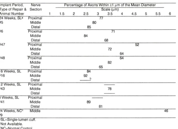
The fiber diameter histograms of the controls and the single-lumen nerve repairs for the four time periods were plotted as percentage of total axons measured versus the axon core diameter. The axon distributions were determined for the proximal, the middle, and the distal sections for each animal. Small axons less than 1 µm in diameter were not represented in the histograms. Also, the total percentage of axons within ± 1 µm of the mean axon diameter in each section was tabulated.
3.4 Statistical Methods
24
4. RESULTS
4.1 Microstructure
The normal control sections and the proximal, middle, and distal cross-sections of the regenerated nerves (8, 12, 16, and 24 week periods) observed using LM have been described by Daniel (1 991) . In the present study, these nerve specimens were also observed using the SEM.
The secondary electron image of an undamaged normal control is shown in Figure 4.1 . The surfaces of axons were covered with the adhesive (Acrytol) remaining after removal of the glass cover slip which had been on top of this surface. The axons were not easy to discriminate in this type of image. However, in the backscatter electron images, the backscatter electrons passed through the thin layer of residual adhesive and revealed the underlying silver-stained axons as bright irregular-shaped closely packed structures (Figure 4.2). For this reason, backscatter electron images were the primary type analyzed in the study.
From the backscatter electron images, two general shapes of axons were seen: (1) approximately circular axons (cross section fully stained) which were termed category I axons and (2) elliptical or arcuate shaped axons or stained rim shaped features which were termed category II axons. These features are not seen clearly in LM images. Examples are shown in the SEM image of Figure 4.3.
Figure 4.1 : Secondary electron micrograph of a cross-section of the right sciatic nerve at the mid-thigh level from a normal control, (animal #9, 24 weeks). Bodian stain. Scale bar=10 µm
Figure 4.3: Backscatter electron image of a single-lumen cuff nerve section, (animal #48, middle section, 24 weeks). Category I and category II axons are in the field of view. Bodian stain. Scale bar=10 µm
ex>
29
particles did not seriously interfere with the observations of the axons in the nerve cross sections.
4.1 .1 Control
Figure 4.2 presents a cross sectional view of the sciatic nerve from a normal control rat. The axons of category I and category II were seen. The two types of axons varied in diameter and were closely packed in the nerve bundles. Some blood vessels were seen among the axons.
4.1.2 Proximal section
The structure changed dramatically at the proximal sites for all four time periods. As compared with the normal control, the differences in numbers and sizes of the category I and the category II axons were significant and a relatively larger fraction of the regenerated nerve cross sectional area was covered with connective tissue. Regenerated axons grouped to form microfascicles and axons in the microfascicles were separated by the connective tissue (Figure 4.5).
4.1.3 Middle section
Figure 4.5: Backscatter electron image of a single-lumen cuff nerve section, (animal #6, proximal section, 24 weeks). Microfascicles are apparent. Category I and category II axons are seen. Bodian stain. Scale bar=10 µm
32
4.1.4 Distal section
The structural differences were not significant at the distal section as compared to the proximal and middle sections (Figure 4.7) .
4.2 Fiber diameter histograms
The fiber diameter histograms for the experimental and the control sections for the four time periods are shown in Appendix. They are designated LM or SEM analyses for the particular animals of Table 3.1 .
Four low-resolution LM micrographs were too obscure to permit analyses of the regenerated axons. They included one from the proximal section of 8 weeks post-implantation nerve, two from the proximal and distal sections of 12 weeks post-implantation nerve, and one from the distal section of 16 weeks post-implantation nerve.
In backscatter electron micrographs, category I and category II axon size distributions were determined. In addition, the two types of axons were combined to obtain the total axon fiber diameter histograms for the various sections.
Table 4.1: Distributions of percentage of axons within ±1 µm of the mean diameter observed using LM
Implant Period, Nerve Percentage of Axons Within ±1 µm of the Mean Diameter
Type of Repair & Section Scale (µm)
Animal Number 1 1.5 2 2.5 3 3.5 4 4.5 5 5.5 6
24 Weeks, SLa Proximal 77
#5 Middle 80
Distal 85
#6 Proximal 71
Middle 84
Distal 68
#47 Proximal 52
Middle 72
Distal 64
#48 Proximal 64
Middle 82 c.v
Distal 65 01
16 Weeks, SL Proximal
84
#16 Middle 92
Distal b
12 Weeks, SL Proximal
#43 Middle 78
Distal
8 Weeks, SL Proximal
#41 Middle 89
Distal 81
24 Weeks, Nee Middle 46
#9
aSL=Single-lumen cuff. bNot Available.
Table 4.2: Distributions of percentage of category I axons within ±1 µm of the mean diameter observed using SEM
Implant Period, Nerve Type of Repair & Section Animal Number
24 Weeks, SLa Proximal
#5 Middle
Distal
#6 Proximal
Middle Distal
#47 Proximal
Middle Distal
#48 Proximal
Middle Distal 16 Weeks, SL Proximal
#16 Middle
Distal 12 Weeks, SL Proximal
#43 Middle
Distal 8 Weeks, SL Proximal
#41 Middle
Distal 24 Weeks, NCb Middle #9
asL=Single-lumen cuff. bNC=Normal Control.
1 1.5
Percentage of Axons Within ±1 µm of the Mean Diameter Scale (µm)
2 2.5 3 3.5 4 4.5 5 5.5
Table 4.3: Distributions of percentage of category II axons within ±1 µm of the mean diameter observed using SEM
Implant Period, Type of Repair & Animal Number 24 Weeks, SL a #5
#6
#47
#48
16 Weeks, SL #16
12 Weeks, SL #43
8 Weeks, SL #41 Nerve Section Proximal Middle Distal Proximal Middle Distal Proximal Middle Distal Proximal Middle Distal Proximal Middle Distal Proximal Middle Distal Proximal Middle Distal
24 Weeks, NCb Middle
#9
aSL=Single-lumen cuff. bNC=Normal Control.
Percentage of Axons Within ±1 µm of the Mean Diameter Scale (µm)
1 1.5 2 2.5 3 3.5 4 4.5 5 5.5
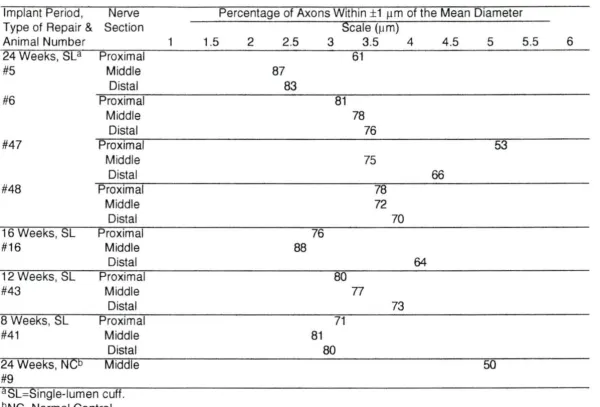
Table 4.4: Distributions of percentage of total axons within ±1 µm of the mean diameter observed using SEM
Implant Period, Nerve Percentage of Axons Within ±1 µm of the Mean Diameter
Type of Repair & Section Scale (µm)
Animal Number 1 1.5 2 2.5 3 3.5 4 4.5 5 5.5 6
24 Weeks, SL a Proximal 61
#5 Middle 87
Distal 83
#6 Proximal 81
Middle 78
Distal 76
#47 Proximal 53
Middle 75
Distal 66
#48 Proximal 78
Middle 72 cu
Distal 70 Q)
16 Weeks, SL Proximal 76
#16 Middle 88
Distal 64
12 W eeks, SL Proximal 80
#43 Middle 77
Distal 73
8 Weeks, SL Proximal 71
#41 Middle 81
Distal 80
24 Weeks, NCb Middle 50
#9
39
4.2.1 Fiber diameter histograms observed using LM
4.2.1.1 Eight Weeks
The fiber diameter histograms were generated for the single lumen nerve cuff experiment for one animal. More than 80% of the middle and the distal distributions were at diameters within ±1 µm of their mean diameters. A larger peak occurred at 3.5 µm in the distal distributions as compared to that occurring at 2.5 µm in the middle distributions.
4.2.1.2 Twelve Weeks
The fiber diameter histograms were generated for the single lumen nerve cuff experiment for one animal. The middle distribution in the group was between 1.5 to 8 µm and exhibited a skewed distribution, with a peak occurring at 3.0 µm. Approximately 78% of the middle distributions were within ±1 µm of the mean diameter.
4.2.1.3 Sixteen Weeks
40
4.2.1.4 Twenty-Four Weeks
The fiber diameter histograms were generated for four single lumen nerve cuff experimental animals and for one normal control animal. In the cuff experiments, the proximal distributions for all the four animals were located at somewhat larger diameters, as compared to the middle and distal distributions. More than 60% of the distributions at the three nerve sections in each animal were within ±1 µm of their mean diameters except in the proximal section of animal #4 7. The normal control animal data showed a bimodal distribution with peaks occurring at 4.0 and 5.0 µm and more than 80% of the axons were located between 2.5 and 8.5 µm. Only 46% of the axons were within ±1 µm of the mean diameter.
4.2.2 Fiber diameter histograms observed using SEM
4.2.2.1 Eight Weeks
41
more than 70% of the axon distributions were within ±1 µ m of their mean diameters.
4.2.2.2 Twelve Weeks
The fiber diameter histograms were generated for the single lumen nerve cuff experiment for one animal. In the category I axon group, the peak in the distal distributions were located at a larger diameter (3.5 µm) as compared to the middle and proximal distributions. More than 50% of the proximal distribution occurred at the smaller diameters (between 2.5 and 3 µm), with the middle distributions located between the proximal and distal distributions. In the category II axon group, no diameters smaller than 2.0 µm occurred in the middle and distal distributions. A larger peak was located at 3.5 µm in the distal section in contrast to the proximal and middle sections. In the total axon group, the distal distributions were located at larger diameters (between 3.5 and 4.5 µm), as compared to the proximal and middle distributions. More than 70% of the distributions for the three axon groups in each nerve section were within ±1 µm of their mean diameters.
4.2.2.3 Sixteen Weeks
42
distributions for the three axon groups in each nerve section were within ±1 µ m of their mean diameters.
4.2.2.4 Twenty-Four Weeks
The fiber diameter histograms were generated for four single lumen nerve cuff experimental animals and for one normal control animal. In the cuff experiments, the proximal distributions of the category I axon group were located between 2.0 and 9.5 µm in animal #47 (a wide spread), and between 1.0 and 7.0 µm in the three other animals. The proximal distributions of all the four animals were located at larger diameters between 3.0 and 4.5 µm as compared to the middle and distal distributions. In the category II axon group, the distributions at the three sections showed skewed distributions toward the smaller sizes. A wide diameter distribution from 1.5 to 10.5 µm also occurred in animal #47. In the total axon group, the proximal and distal distributions occurred at larger diameters (between 2.0 and 4.5 µm) and the middle distributions were located at the smaller diameters (between 2.0 to 3.0 µm). More than 60% of the distributions for the three axon groups in each of the three nerve sections were within ±1 µm of their mean diameters, except in the proximal section of animal #47.
43
4.3 Quantitative results
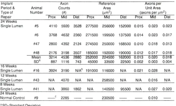
The quantitative data were obtained from light and scanning electron micrographs. It should be noted that in the normal control animal, the quantitative data were obtained from sections taken from only one site in the sciatic nerve which was comparable to the middle of the repair site in the single-lumen cuff repaired nerves since the separation was only at one location. Four low-resolution LM micrographs as described before were not studied in the quantitative evaluations. In the SEM micrographs, the category I and the category II axons were used for the quantitative study. Moreover, the total axons which combined the two types of axons were also studied. The quantitative results are shown in Table 4.5 through Table 4.16. Table 4.5 to Table 4 .8 list the axon counts, reference area, and axons per unit area observed using LM and SEM. Table 4.9 to Table 4.12 list the mean axon diameter, nerve area, and percentage of nerve observed using LM and SEM. Table 4.13 to Table 4.16 list the axon diameter ratio and estimated total number of axons in each nerve cross section observed using LM and SEM. The results in these tables are grouped according to the nerve sites examined and to the implantation periods. Means and standard deviations are also presented.
Table
4.5:
Axon counts, reference area and axons per unit area observed using LMImplant Axon Reference Axons per
Period & Animal Counts Area Unit Area
Type of Number
(#)
(µm2) (axons per µm2)Repair Prox Mid Dist 15rox Mid Dist Prox Mid Dist
24
WeeksSingle Lumen
#5
4110 5920 3528 277500 256000 152000 0.015 0.023 0.023
#6
3768 4632 2360 271500 199500 137500 0.014 0.023 0.017
#47
2800 4392 2124 274500 250000 168500 0.010 0.018 0.013
#48
2176 3198 3507 185000 192000 190000 0.012 0.017 0.018
Mean
3214 4536 2880 252000 224500 162000 0.013 0.020 0.018
soa
887 1116 743
45000
33500
22500 0.002 0.003 0.004
16
WeeksSingle Lumen
#16
3924 3190
NI
Ab191000 116000
NIA
0.021 0.028
NIA
12
WeeksSingle Lumen
#43
NIA
4070
NIA NIA
258500
NIA
NIA
0.016
NIA
8
WeeksSingle Lumen
#41
NIA
3860 1862
NIA
140500 95500
NIA
0.027 0.020
24
WeeksNormal Control
#9
- c2285
230500
0.010
a
SD=Standard Deviation. bNot Available. [image:51.776.98.678.82.431.2]Table
4.6:
Category I axon counts, reference area and category I axons per unit area observed using SEMImplant Axon Reference Axons per
Period & Animal Counts Area Unit Area
Type of Number
(#)
(µm2) (axons per µm2)Repair Prox Mid Dist Prox Mid Dist Prox Mid l>ist
24
WeeksSingle Lumen
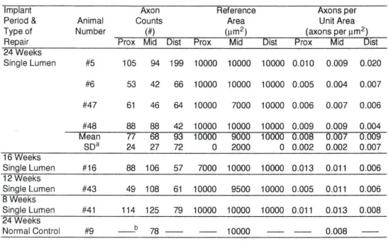
#5
105
94199 10000 10000 10000 0.010 0.009 0.020
#6
53 42 66 10000 10000 10000 0.005 0.004 0.007
#47
61
46
6410000 7000 10000 0.006 0.007 0.006
#48
88 8842 10000 10000 10000 0.009 0.009 0.004
Mean 77 68
93 10000 9000 10000 0.008 0.007 0.009
~ 01soa
24 27 72
0 2000
0 0.002 0.002 0.007
16
WeeksSingle Lumen
#16
88 106 57 7000 10000 10000 0.013 0.011 0.006
12
WeeksSingle Lumen
#43
49 108 61 10000 9500 10000 0.005 0.011 0.006
8
WeeksSingle Lumen
#41
114 125 79 10000 10000 10000 0.011 0.013 0.008
24
WeeksNormal Control
#9
b 7810000
0.008
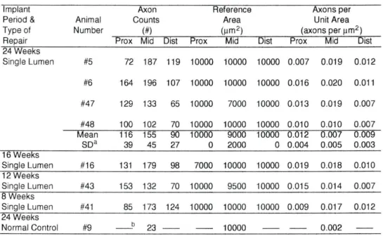
[image:52.781.96.643.96.435.2]Table 4.7: Category II axon counts, reference area and category II axons per unit area observed using SEM
Implant Axon Reference Axons per
Period & Animal Counts Area Unit Area
Type of Number (#) (µm 2) (axons per µm2 )
Repair Prox Mid Dist Prox Mid Dist Prox Mid i:5ist 24 Weeks
Single Lumen #5 72 187 119 10000 10000 10000 0.007 0.019 0.012
#6 164 196 107 10000 10000 10000 0.016 0.020 0.011
#47 129 133 65 10000 7000 10000 0.013 0.019 0.007
#48 100 102 70 10000 10000 10000 0.010 0.010 0.007 ~
Mean 116 155 90 10000 9000 10000 0.012 0.007 0.009 (J') SD a 39 45 27 0 2000 0 0.004 0.005 0.003
16 Weeks
Single Lumen #16 131 179 98 7000 10000 10000 0.019 0.018 0.010 12 Weeks
Single Lumen #43 153 132 70 10000 9500 10000 0.015 0.014 0.007 8 Weeks
Single Lumen #41 85 173 124 10000 10000 10000 0.009 0.017 0.012 24 Weeks
Normal Control #9 b 23 10000 0.002
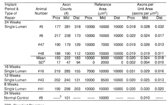
Table 4.8: Total axon counts, reference area and axons per unit area observed using SEM
Implant Axon Reference Axons per
Period & Animal Counts Area Unit Area
Type of Number (#) (µm2) (axons per µm2)
Repair Prox Mid Dist Prox Mia Dist Prox Mid i:>ist
24 Weeks
Single Lumen #5 177 281 318 10000 10000 10000 0.018 0.028 0.032
#6 217 238 173 10000 10000 10000 0.022 0.024 0.017
#47 190 179 129 10000 7000 10000 0.019 0.026 0.013
#48 188 190 112 10000 10000 10000 0.019 0.019 0.011
Mean 193 222 183 10000 9000 10000 0.020 0.024 0.018 ~
soa 17 47 94 0 2000 0 0.002 0.004 0.010 -.._J
16 Weeks
Single Lumen #16 219 285 155 7000 10000 10000 0.031 0.029 0.016
12 Weeks
Single Lumen #43 202 240 131 10000 9500 10000 0.020 0.025 0.013
8 Weeks
Single Lumen #41 199 298 203 10000 10000 10000 0.020 0.030 0.020
24 Weeks
Normal Control #9 - b 101 10000 0.010
[image:54.776.84.642.78.425.2]Table
4.9:
Mean axon diameter, nerve area and percentage of nerve observed using LMImplant Mean Axon Diameter Nerve Area Percentage of
Period & Animal
±
Standard Deviation (µm2) Nerve ExaminedType of Number (um) (%)
Repair Prox Mid Dist Prox Mid Dist Prox Mid Dist
24
WeeksSingle Lumen
#5
3.2±1.0 2.7±1.0 2.6±1 .0 1180000 550000 380000 24 47
40#6
3.6±1.3 2.5±0.9 3.3±1 .2 570000 510000 910000
4839 15
#47
4.6±1.7 3.5±1.1 3.9±1.3 670000 470000 530000 41
5332
#48
4.0±1.4 3.5±1 .0 3.2±1 .2 800000 510000 710000 23 38 27
Mean3.9
3.1
3.2
805000 510000 632500
34 4429
SD a
1.5
1.1
1.2
267000 32500 229000 12
7 10
~CX)
16
WeeksSingle Lumen
#16
2.6±0.9 2.5±0.8
N/Ab370000 380000 1110000 52 31
N/A12
WeeksSingle Lumen
#43
N/A3.5±1.1
N/A700000 510000 1410000
N/A51
N/A8
WeeksSingle Lumen
#41
N/A2.6±0.9 3.2±1 .1 130000 480000 770000
N/A29
12
24
WeeksNormal Control
#9
- c5.7±1 .9
520000
44a SD=Standard Deviation. bNot Available.
[image:55.783.100.689.84.429.2]Table 4.10: Mean category I axon diameter, nerve area and percentage of nerve observed using SEM
Implant Mean Axon Diameter Nerve Area Percentage of
Period & Animal ± Standard Deviation (µm2) Nerve Examined
Type of Number (um) (%)
Repair Prox Mid Dist Prox Mid Dist Prox Mid Dist
24 Weeks
Single Lumen #5 3.4±1.2 2.4±0.8 2.2±0.9 1180000 550000 380000 1 2 3
#6 2.9±0.8 2.8±0.9 3.5±0.9 570000 510000 910000 2 2 1
#47 4.9±1.6 3.6±0.9 3.8±1.0 670000 470000 530000 1 1 2
#48 3.5±0.9 3.6±1.2 3.6±1 .1 800000 510000 710000 1 2 1
Mean 3.9 3.o 3.1 805000 510000 632500 1 2 2
SD a 1.5 1.1 1.2 267000 32500 229000 1 1 1 <D ~
16 Weeks
Single Lumen #16 2.7±0.8 2.4±0.7 4.0±1.2 370000 380000 1110000 2 3 1
12 Weeks
Single Lumen #43 3.0±0.8 3.1±1 .0 3.8±1.1 700000 510000 1410000 1 2 1
8 Weeks
Single Lumen #41 3.1±1.4 2.9±1.0 2.9±0.8 130000 480000 770000 8 2 1
24 Weeks
Normal Control #9 - b 5.1±1.8 520000 2
Table 4.11 : Mean category II axon diameter, nerve area and percentage of nerve observed using SEM
Implant Mean Axon Diameter Nerve Area Percentage of
Period & Animal ± Standard Deviation (µm2) Nerve Examined
Type of Number (um) (%)
Repair Prox Mid Dist Prox Mid Dist Prox Mid Dist
24 Weeks
Single Lumen #5 3.2±1.3 2.3±0.8 2.7±0.8 1180000 550000 380000 1 2 3
#6 3.3±1.0 3.4±1.1 3.4±1.1 570000 510000 910000 2 2 1
#47 5.3±1.6 3.5±1.1 4.7±1.4 670000 470000 530000 1 1 2
#48 3.6±1.1 3.6±1.1 4.0±1.1 800000 510000 710000 1 2 1
Mean 4.2 3.1 3.8 805000 510000 632500 1 2 2
SD a 1.6 1.1 1.3 267000 32500 229000 1 1 1 (JI 0
16 Weeks
Single Lumen #1 6 3.0±1.1 2.8±0.8 4.1±1.4 370000 380000 1110000 2 3 1
12 Weeks
Single Lumen #43 3.3±1.0 3.4±0.9 4.1±1.2 700000 510000 1410000 1 2 1
8 Weeks
Single Lumen #41 3.5±1.0 2.9±1.0 3.2±1.1 130000 480000 770000 8 2 1
24 Weeks
Normal Control #9 - b 4.9±1 .6 520000 2
Table 4.12: Mean total axon diameter, nerve area and percentage of nerve observed using SEM
Implant Mean Axon Diameter Nerve Area Percentage of
Period & Animal ± Standard Deviation (µm2) Nerve Examined
Type of Number (um) (%)
Repair Prox Mid Dist Prox Mid Dist Prox Mid Dist
24 Weeks
Single Lumen #5 3.3±1.3 2.3±0.8 2.4±0.9 1180000 550000 380000 1 2 3
#6 3.2±1.0 3.3±1.1 3.4±1.0 570000 510000 910000 2 2 1
#47 5.2±1.6 3.5±1.1 4.3±1.3 670000 470000 530000 1 1 2
#48 3.6±1.0 3.6±1.1 3.8±1.1 800000 510000 710000 1 2 1
Mean 4.1 3.1 3.4 805000 510000 632500 1 2 2
SD a 1.6 1.1 1.3 267000 32500 229000 1 1 1 01 ...
16 Weeks
Single Lumen #16 2.9±1.0 2.6±0.8 4.1±1.3 370000 380000 1110000 2 3 1
12 Weeks
Single Lumen #43 3.2±1.0 3.3±1.0 3.9±1.1 700000 510000 1410000 1 2 1
8 Weeks
Single Lumen #41 3.2±1.3 2.9±1.0 3.1 ±1.0 130000 480000 770000 8 2 1
24 Weeks
Normal Control #9 - b 5.0±1.7 520000 2
Table 4.13: Diameter ratio and estimated total axons in each nerve cross section observed using LM
Implant Diameter Ratio ± Axon
Period & Animal Standard Deviation Counts
Type of Number (#)
Repair Prox Mid Dist Prox Mid Dist
24 Weeks
Single Lumen #5 1.6±0.6 2.0±0.9 1.4±0.4 17125 12596 8820
#6 1.8±0.7 1.6±0.7 1.8±0.6 7850 11877 15733
#47 1.5±0.5 1.8±0.8 1.7±0.5 6829 8287 6638
#48 1.7±0.7 1.6±0.4 1.4±0.4 9461 8416 12989
Mean 10316 10294 11045
SD a b 4667 2263 4088 Ul
I\) 16 Weeks
Single Lumen #16 1.8±0.7 1.6±0.5 N/Ac 7546 10290 N/A
12 Weeks
Single Lumen #43 N/A 1.9±0.8 N/A N/A 7980 N/A
8 Weeks
Single Lumen #41 N/A 1.5±0.5 1.7±0.7 N/A 13310 15517
24 Weeks
Normal Control #9 1.7±0.7 5193
a SD=Standard Deviation. bNot Applicable.
Table 4.14: Category I axon diameter ratio and estimated total category I axons in each neNe cross section obseNed using SEM
Implant Diameter Ratio ± Axon
Period & Animal Standard Deviation Counts
Type of Number (#)
Repair Prox Mid Dist Prox Mid Dist
24 Weeks
Single Lumen #5 1.6±0.5 1.7±0.6 1.6±0.6 10500 4700 6633
#6 1.6±0.5 1.6±0.6 1.8±0.6 2650 2100 6600
#47 1.4±0.3 1.7±0.5 1.6±0.6 6100 4600 3200
#48 1.7±0.6 2.0±0.7 1.5±0.5 8800 4400 4200
Mean 7013 3950 5158 01
(,.)
soa
b 3426 1240 173316 Weeks
Single Lumen #16 1.8±0.9 2.0±1.1 1.6±0.5 4400 3533 5700
12 Weeks
Single Lumen #43 1.5±0.4 1.6±0.6 1.9±0.8 4900 5400 6100
8 Weeks
Single Lumen #41 1.8±0.9 1.4±0.3 1.9±0.7 1425 6250 7900
24 Weeks
Normal Control #9 1.7±0.5 3900
Table 4.15: Category II axon diameter ratio and estimated total category II axons in each nerve cross section observed using SEM
Implant Diameter Ratio ± Axon
Period & Animal Standard Deviation Counts
Type of Number (#)
Repair Prox Mid Dist Prox Mid Dist
24 Weeks
Single Lumen #5 1.5±0.3 1.6±0.5 1.4±0.5 7200 9350 3967
#6 1.3±0.2 1.3±0.2 1.5±0.4 8200 9800 10700
#47 1.5±0.5 1.7±0.6 1.5±0.4 12900 13300 3250
#48 1.5±0.4 1.8±0.5 1.6±0.5 10000 5100 7000
Mean 9575 9388 6229 01
~
SD a b 2501 3360 3395
16 Weeks
Single Lumen #16 1.4±0.4 1.6±0.5 1.5±0.5 6550 5967 9800
12 Weeks
Single Lumen #43 1.6±0.5 1.5±0.3 1.6±0.8 15300 6600 7000
8 Weeks
Single Lumen #41 1.6±0.5 1.5±0.5 1.4±0.4 1063 8650 12400
24 Weeks
Normal Control #9 1.7±0.4 1150
Table 4.16: Axon diameter ratio and estimated total axons in each nerve cross section observed using SEM
Implant Diameter Ratio ± Axon
Period & Animal Standard Deviation Counts
Type of Number (#)
Repair Prox Mid Dist Prox Mid Dist
24 Weeks
Single Lumen #5 1.6±0.4 1.6±0.5 1.5±0.6 17700 14050 10600
#6 1.4±0.3 1.4±0.4 1.6±0.5 10850 11900 17300
#47 1.4±0.4 1.7±0.6 1.6±0.5 19000 17900 6450
#48 1.6±0.5 1.9±0.6 1.6±0.5 18800 9500 11200
Mean 16588 13338 11388 01
01
soa b 3867 3564 4472
16 Weeks
Single Lumen #16 1.6±0.7 1.8±0.8 1.5±0.5 10950 9500 15500
12 Weeks
Single Lumen #43 1.6±0.5 1.5±0.5 1.7±0.8 20200 12000 13100
8 Weeks
Single Lumen #41 1.7±0.8 1.5±0.4 1.6±0.6 2488 14900 20300
24 Weeks
Normal Control #9 1.7±0.5 5050
56
not the mean differences were significant for each type of axon in the three neNe sections in each animal. For each section in repaired nerves, the means of the two types of axons were compared, respectively, with those in the normal control. In addition, the means of the total axons obtained in the three sections in each repaired neNe were compared with each other as well as with the normal control. Finally, the means of the total axons obseNed using SEM were compared with those obtained using LM in the present study. The statistical comparisons can be seen in Table 4.17 through Table 4.24.
4.3.1 Quantitative results from LM
Approximately 30 to 50 percent of areas in each neNe section were analyzed. The Tukey's test showed that all sections tested from the single-lumen cuff repaired neNes over the four time periods had significantly lower mean axon core diameters than the normal control (Table 4.17). Among the three sections of the 24 week post-implantation neNe cases, the axon core diameters were the largest at the proximal sites as compared to the middle and distal sections (Table 4.18). However, the mean core diameter of the regenerated axons did not reach the normal control level size even after 24 weeks.
57
Table 4.17: Mean axon diameter comparisons between repaired nerve sections and normal control observed using LM
Animal Type of Repair Implant Section Significanceb
Number Periods Comparisons a
#41 Single-lumen 8 Weeks p N/A
M ••• (p<0.0001) (+)
D *** (p<0.0001) (+)
#43 Single-lumen 12Weeks p N/A
M *** (p<0.0001) (+)
D N/A
#16 Single-lumen 16 Weeks p *** (p<0.05) (+)
M *** (p<0.05) (+)
D N/A
#5 Single-lumen 24 Weeks p ••• (p<0.0001) (+)
M *** (p<0.0001) (+) D *** (p<0.0001) (+)
#6 Single-lumen 24 Weeks p *** (p<0.0001) (+)
M *** (p<0.0001) (+) D *** (p<0.0001) (+)
#47 Single-lumen 24 Weeks p *** (p<0.0001) (+)
M *** (p<0.0001) ( +) D *** (p<0.0001) (+)
#48 Single-lumen 24 Weeks p *** (p<0.0001) (+)
M *** (p<0.0001 ) (+) D *** (p<0.0001 ) (+) aP=Proximal; M=Middle; D=Distal; Comparing the sections with normal control. bN/A=Not Available;(+) Larger mean axon diameters in normal control.
58
Table 4.18: Mean axon diameter comparisons between nerve sections in the same animal observed using LM
Animal Type of Implant Section Signiticanceb
Number Repair Periods Comparisons a
#41 Single-lumen 8 Weeks P, M N/A
P, D N/A
M, D *** (p<0.0001) (-)
#43 Single-lumen 12 Weeks P, M N/A
P, D N/A
M, D N/A
#16 Single-lumen 16 Weeks P, M *** (p<0.01) (+)
P,D N/A
M, D N/A
#5 Single-lumen 24 Weeks P, M *** (p<0.0001) (+)
P,D *** (p<0.0001) (+)
M,D *
#6
Single-lumen 24 Weeks P,M *** (p<0.0001) (+)P, D *** (p<0.0001) (+) M,D *** (p<0.0001) (-)
#47 Single-lumen 24 Weeks P, M *** (p<0.001) (+)
P, D *** (p<0.001) (+) M, D *** (p<0.001) (-)
#48 Single-lumen 24 Weeks P, M *** (p<0.0001) (+)
P, D *** (p<0.0001) (+) M, D *** (p<0.0001) (+) aP=Proximal; M=Middle; D=Distal.
bN/A=Not Available; (+) Larger mean axon diameters in the first nerve section; (-) Larger mean axon diameters in the second nerve section.
59
Table 4.19: Mean diameter comparisons of the same category of axons in repaired nerve sections and in normal control observed using SEM
Animal Type of Implant Nerve Axon Significancec
Number Repair Periods Sectiona Comparisonsb
#41 Single-lumen 8 Weeks p I *** (p<0.05) (+)
p II *** (p<0.05) (+)
M I *** (p<0.05) (+)
M II *** (p<0.05) (+)
D I *** (p<0.05) (+)
D II *** (p<0.05) (+)
#43 Single-lumen 12 Weeks p I *** (p<0.05) (+)
p II *** (p<0.05) (+)
M I *** (p<0.05) (+)
M II *** (p<0.05) (+)
D I *** (p<0.05) (+)
D II *
#16 Single-lumen 16 Weeks p I *** (p<0.05) (+)
p II *** (p<0.05) (+)
M I *** (p<0.05) (+)
M II *** (p<0.05) (+)
D I *** (p<0.05) (+)
D II *** (p<0.05) (+)
a P=Proximal; M=Middle; D=Distal.
bl=Category I axons; ll=Category II axons; Comparing axons in the nerve sections with those in normal control.
c(+) Larger mean axon diameters in normal control.
60
Table 4.19: Continued
Animal Type of Implant Nerve Axon Signiticancec Number Repair Periods Section8 Comparisonsb
#5 Single-lumen 24 Weeks p I *** (p<0.01) (+)
p II *** (p<0.01) (+) M I *** (p<0 .01) (+) M II *** (p<0.01) (+) D I ••• (p<0 .01) (+) D II *** (p<0.01) (+)
#6
Single-lumen 24 Weeks p I ... (p<0.01) ( +)p II ••• (p<0.01) (+) M I ••• (p<0.01) (+) M II ••• (p<0 .01) (+) D I ••• (p<0.01) (+) D II ••• (p<0.01) (+)
#47 Single-lumen 24 Weeks p I *
p II •
M I ••• (p<0.0001) (+) M II ••• (p<0.0001) (+) D I ••• (p<0.0001) (+)
D II *
#48 Single-lumen 24 Weeks p I ••• (p<0.05) (+)
61
Table 4.20: Mean axon diameter comparisons between repaired nerve sections and normal control observed using SEM
Animal Type of Implant Section Significance b
Number Repair Periods Comparisonsa
#41 Single-lumen 8 Weeks p *** (p<0.0001) (+)
M *** (p<0.0001) (+)
D *** (p<0.0001) (+)
#43 Single-lumen 12 Weeks p *** (p<0.0001) (+)
M *** (p<0.0001 ) (+)
D *** (p<0.0001 ) (+)
#16 Single-lumen 16 Weeks p *** (p<0.0001 ) (+)
M *** (p<0.0001 ) (+)
D *** (p<0.0001 ) (+)
#5 Single-lumen 24 Weeks p *** (p<0.0001) (+)
M *** (p<0.0001) (+)
D *** (p<0.0001) (+)
#6 Single-lumen 24 Weeks p *** (p<0.0001) (+)
M *** (p<0.0001) (+)
D *** (p<0.0001 ) (+)
#47 Single-lumen 24 Weeks p *
M *** (p<0.0001 ) (+)
D *** (p<0.0001 ) (+)
#48 Single-lumen 24 Weeks p *** (p<0.0001 ) (+)
M *** (p<0.0001 ) (+)
D *** (p<0.0001 ) (+)
aP=Proximal; M=Middle; D=Distal; Comparing the sections with normal control.
b(+) Larger mean axon diameters in normal control.
***Comparisons significant at the 0.05 level, p value in brackets.
62
Table 4.21 : Diameter comparisons between the category I and the category II axons in the same nerve section observed using SEM
Animal Type of Implant Nerve Significanceb
Number Repair Periods Section a
#41 Single-lumen 8 Weeks p •
M •
D •
#43 Single-lumen 12Weeks p •
M •
D •
#16 Single-lumen 16 Weeks p •
M •
D •
#5 Single-lumen 24 Weeks p •
M •
D ••• (p<0.05) (+)
#6 Single-lumen 24 Weeks p •
M •
D •
#47 Single-lumen 24 Weeks p •
M •
D ••• (p<0.0001) (+)
#48 Single-lumen 24 Weeks p •
M •
D •
#9 Normal Control 24 Weeks M •
aP=Proximal; M=Middle; D=Distal.
b(+) Larger mean axon diameters in category II axons.
63
Table 4.22: Mean diameter comparisons of the same category of axons in different nerve sections observed using SEM
Animal Type of Implant Section Axon Significance c
Number Repair Periods Comparisons a Typeb
#41 Single-lumen 8 Weeks P, M I *
P, M II *** (p<0.05) (+)
P, D I *
P, D II *
M, D I *
M, D II *
#43 Single-lumen 12 Weeks P, M I *
P, M II *
P, D I *** (p<0.05) (-)
P, D II *** (p<0.05) (-)
M,D I *** (p<0.05) (-)
M,D II *** (p<0.05) (-)
#16 Single-lumen 16 Weeks P, M I *
P,M II *
P, D I *** (p<0.05) (-)
P, D II *** (p<0.05) (-)
M, D I *** (p<0.05) (-)
M, D II *** (p<0.05) (-)
a P=Proximal; M=Middle; D=Distal.
b l=Category I axons; I !=Category 11 axons.
c(+) Larger mean axon diameters in the first nerve section; (-) Larger mean
axon diameters in the second nerve section.
64
Table 4.22: Continued
Animal Type of Implant Section Axon Significancec
Number Repair Periods Comparisonsa Typeb
#5 Single-lumen 24 Weeks P,M I ••• (p<0.01) (+)
P,M II ••• (p<0.01) (+)
P, D I ••• (p<0.01) (+)
P,D II *** (p<0.01) (+)
M, D I *
M,D II *
#6
Single-lumen 24 Weeks P, M I *P,M II *
P, D I *** (p<0.01) (-)
P, D II *
M, D I *** (p<0.01) (-)
M, D II *
#47 Single-lumen 24 Weeks P, M I ••• (p<0.0001) (+)
P,M II *** (p<0.0001) (+)
P,D I ••• (p<0.0001) (+)
P,D II *** (p<0.0001) (+)
M, D I *
M,D II ••• (p<0.0001) (-)
#48 Single-lumen 24 Weeks P, M I *
P, M II *
P, D I *
P, D II *
M, D I *
65
Table 4.23: Mean diameter of total axons comparisons between nerve sections in the same animal observed using SEM
Animal Type of Implant Section Significanceb
Number Repair Periods Comparisons a
#41 Single-lumen 8 Weeks P, M ••• (p<0.0001) (+)
P, O *
M, O •
#43 Single-lumen 12 Weeks P, M •
P, O ••• (p<0.0001) (-) M, O ••• (p<0.0001) (-)
#16 Single-lumen 16 Weeks P, M •
P, O *** (p<0.0001) (-) M, O ••• (p<0.0001) (-)
#5 Single-lumen 24 Weeks P, M ••• (p<0.0001) (+)
P, O ••• (p<0.0001) (+)
M, O •
#6
Single-lumen 24 Weeks P, M •P, O •
M, O *
#47 Single-lumen 24 Weeks P, M ••• (p<0.0001) (+)
P, O .... (p<0.0001) (+)
M, O *** (p<0.0001) (-)
#48 Single-lumen 24 Weeks P, M *
P, O *
M, O *
a P=Proximal; M=Middle; D=Distal.
b(+) Larger mean axon diameters in the first nerve section; (-) Larger mean axon diameters in the second nerve sections.