Low-complexity energy disaggregation using appliance load modelling

http://www.aimspress.com/journal/energy

DOI: 10.3934/energy.2016.1.1 Received: 26 October 2015, Accepted: 23 December 2015, Published: 05 January 2016

Research article

Low-complexity energy disaggregation using appliance load modelling

Hana Altrabalsi, Vladimir Stankovic, Jing Liao∗_{and Lina Stankovic}

Department of Electronic and Electrical Engineering, University of Strathclyde, Glasgow, UK

∗

Correspondence: Email: [email protected]; Tel:+44-141-548-2679.

The work was presented in part atIEEE Symposium Series on Computational Intelligence (SSCI)

Applications in Smart Grid, Orlando, FL, December 2014.

Abstract: Large-scale smart metering deployments and energy saving targets across the world have ignited renewed interest in residential non-intrusive appliance load monitoring (NALM), that is, disag-gregating total household’s energy consumption down to individual appliances, using purely analytical

tools. Despite increased research efforts, NALM techniques that can disaggregate power loads at low

sampling rates are still not accurate and/or practical enough, requiring substantial customer input and

long training periods. In this paper, we address these challenges via a practical complexity low-rate NALM, by proposing two approaches based on a combination of the following machine learning techniques: k-means clustering and Support Vector Machine, exploiting their strengths and addressing their individual weaknesses. The first proposed supervised approach is a low-complexity method that requires very short training period and is fairly accurate even in the presence of labelling errors. The second approach relies on a database of appliance signatures that we designed using publicly available datasets. The database compactly represents over 200 appliances using statistical modelling of mea-sured active power. Experimental results on three datasets from US, Italy, Austria and UK, demonstrate the reliability and practicality.

Keywords: energy disaggregation; appliance modelling; non-intrusive appliance load monitoring

1. Introduction

Large scale deployment of smart meters for residential customers is well underway in many Eu-ropean and other countries. For example, it is anticipated that by 2020 all UK households who give their permission will be equipped with an automatic meter reading system that measures and displays in real time aggregate energy usage with an home display unit [1]. This large governmental

in-vestment promises significant improvements in energy demand via automatic, more efficient and more

in-dividual appliance is necessary. Indeed, up to 20% of reduction in energy consumption is expected via appliance-feedback and specific appliance replacement programs [2].

Monitoring individual appliances using individual appliance-specific sensors in a house is often impractical and expensive, especially since the number of electrical devices in the home is rapidly increasing. On the other hand, energy disaggregation via non-intrusive appliance load monitoring

(NALM) offers a non-intrusive, purely computational, software-based approach to separate aggregate

load obtained from a single electricity meter into individual appliance loads.

NALM appeared in the research literature in the 1980’s [3], and since then, many NALM algorithms have been proposed that improve the initial design of [3] and adapt to advances in sensor technology, capturing energy measurands at a range of sampling rates, generally in the order of kHz. See [2, 4, 5, 6, 7], for examples of NALM applications. However, with large-scale smart metering deployments on the way, there is an increased interest in NALM algorithms that work at lower sampling rates, in the order of seconds and minutes. It is not only the cost of the sensing technology [2], but also computational and

storage cost as well as implementation efficiency that are key drivers towards wide deployment of

low-sampling smart meters. For example, in the USA most utilities capture data at 15-min intervals. UK smart meters, as defined by the Smart Metering Equipment Technical Specification (SMETS) proposal by UK Department of Energy and Climate Change provide readings at 30 min intervals to energy suppliers, but an 8-10 second sampling rate for load readings is available to households that install a Consumer Access Device in their homes to read the smart meter measurements directly [1]. However,

so far, there are no widely available efficient solutions for NALM, that offer high accuracy and low

complexity at such low sampling rates [4, 5].

Based on the requirement for labelled training, all NALM methods can be grouped into supervised and unsupervised techniques (though hybrid, semi-supervised approaches are also possible). Super-vised NALM techniques (see, for example, [8, 9, 10]) require a labelled dataset for training, are com-monly based on event detection, and generally provide the highest disaggregation accuracy. They rely

on different optimization and pattern recognition approaches, such as rule-based, neural networks, or

Bayes-based classification. However, these approaches are less practical and prone to errors since the training usually relies on customer-filled appliance diaries, that are often unreliable.

Unsupervised approaches do not require a labelled dataset for training, and are currently probabilis-tic [11, 12, 13, 14], based on sparse coding [15], or time-series and motif mining [16, 17]. All these approaches, however, still require substantial customer input and depend on the availability of time

periods when only one appliance is running for building efficient probabilistic models [11, 12, 13] or

database of signatures [17].

In this paper, based on our initial conference paper [18], we propose an efficient low-complexity

supervised NALM approach that combines k-means and Support Vector Machine (SVM). In particular, to benefit from the high classification performance of non-linear SVMs and low computational cost of

k-means clustering, we effectively combine conventional k-means and SVM obtaining a hybrid method

select a subset of original data for SVM training. The clustered SVM of [22] trains a linear SVM on each of the k-means clusters, in a divide-and-conquer manner.

To make the above approach practical and reduce or remove customer effort in maintaining a

time-diary, a database of appliance signatures is created. Such a database is then used to develop a novel approach that requires no training from the household, and hence no input from the customer. The designed database is a compact collection of appliance power load signatures (active power measure-ments over a duty cycle) plus statistical features, such as, mean, variance, auto-correlation, and a statistical model for each appliance that are then used for load disaggregation. The database is popu-lated using open source datasets from the USA [23], Austria and Italy [24], and our measurements in 20 UK houses [7]. Similar attempts have recently been reported in [25] but for USA houses only and high sampling rates.

The main contributions of the paper are:

• A low-complexity NALM approach, trained on measurements from the house whose aggregate

load NALM is being applied on; this is termed Approach 1 using House-specific training data;

• A generic database of appliance signatures populated from 34 houses in UK, Europe, and US,

containing over 200 appliance signatures. The database∗can be used with different energy

disag-gregation algorithms as well as for appliance mining and load prediction

• A low-complexity NALM approach that uses the developed database for training, irrespective of

the house, and hence does not require customer input; this is termed Approach 2 using House-agnostic training data.

The developed approaches are tested in real settings using real house measurements. We tested the

supervised approach for different training periods and artificially introduced errors in the training set.

The rest of the paper is organized as follows. Section 2 provides a brief review on NALM. Section 3 describes the proposed NALM algorithms and the database of appliance signatures. The last two sections discuss the simulation results, conclusion and future work.

2. Background and literature review

Non-intrusive Appliance Load Monitoring(NALM), also referred to as NILM or NIALM [3],

dis-aggregates total power readings and identifies each appliance in use at any point in time based on the available measured total household consumption.

Traditional event-based NALM methods [3] consist of signal pre-processing, edge detection and feature extraction followed by classification. After acquisition, signal pre-processing can be done in the form of power normalization, filtering (for signal smoothing and getting rid of sudden peaks), and thresholding to remove small power loads that would appear as noise as well as the base-load, from appliances that are always running. Next, edge detection is done to identify events of appliances

switching on and off. Edge detection is followed by extracting the features in the identified event

win-dows. Classification is then used to group sets of extracted features which have similar characteristics, such as power levels, time profile, reactive components etc.

In this paper, we focus on low complexity, low-rate NALM algorithms, where sampling rates are in the range of seconds and minutes. In particular, we test the proposed methods using 1 sec, 8 sec, and

∗

1 min sampling rates. The sampling rate influences the type of features that can be used. For example, low-rate NALM approaches can use only steady-state parameters, such as active or real power [12], reactive power [3, 4], power factor [26], voltage or current waveform [27, 28].

The simplest approach, from an implementation point of view, is to use a current transformer (CT) sensor with a clamp to measure alternating current and an AC-to-AC power adapter with a circuit to measure voltage. This way, active and reactive power components can be calculated from the mea-sured current and voltage. However, measuring voltage in a simple way requires additional plug points, which are often not available close to the electricity meter. Moreover, processing, communicating and storing two dimensional data (active and reactive power) is often impractical, especially because the reactive component is not needed for billing purposes. That is why, in this paper, we consider disag-gregation using only active power values, obtained, for example, from the electric current measured via a simple CT sensor, which is a type of metering massively deployed for automated meter reading.

Recent work on NALM has mainly focused on state-based probabilistic methods. In [11] four

different methods for low-rate NALM are proposed using (conditional) factorial Hidden Markov Model

(HMM) and Hidden semi-Markov models. The obtained accuracy was in the range of 72% to 99% for

3 sec sampling rate in seven different houses with an average accuracy of 83%. This method cannot

disaggregate base load, that is, the lowest most frequent value extracted from the aggregate load data, which is a good indication of the number of appliances being left on standby or background appliances such as boiler control units, fridges and freezers. The method is not of low computational complexity, and is prone to converge to a local minimum.

In [12] a factorial HMM is used for disaggregation of active power load at 1 min sampling rate. The method builds initial models for state transition probabilities using knowledge of appliance-specific power operation that can be obtained, for example, from study and understanding of the appliance

operation. To obtain reliable results, it is necessary to correctly set thea priori-values for each state

of each appliance, which in turn is strongly dependent on the particular aggregate dataset on which NALM is being performed. Indeed, a similar factorial HMM-based approach is tested in [23], where

it is shown that the disaggregation accuracy drops by up to 25% when different houses are used to set

the initial models compared to the case when the same house is used for building the models (training) and testing. Results are reported for REDD dataset [23] with sampling rates of 1 sec and 3 sec.

In [29] and [8] a decision-tree (DT) classifier is used for pattern matching. The DT-based algorithm developed in [8], is a low-complexity, supervised approach that uses only rising and falling active power edges to build a DT model that is used for classification. The method is not scalable, since re-training is needed whenever a new appliance is added, but is fast and performs very well even when the training period is very short.

In [13], an unsupervised Additive Factorial Approximate Maximum A-Posteriori (AFMAP)

infer-ence algorithm is proposed using differential factorial HMMs. First, all snippets of active power data

are extracted using a threshold and modelled by an HMM; next the k-nearest-neighbor graph is used to build nine motifs that are treated as HMMs over which AFMAP is run. The results show average

accuracy of 87.2% using 7 appliances and sampling rate of 60 Hz. In [14] Hierarchical Dirichlet

A powerful classification technique used for NALM is SVM. SVM-based NALM has shown good performance [5], it is scalable, and is a well established method for classifying noisy data. Non-linear classifiers, such as kernel SVM, that map the input feature space into a high dimensional space and find

the optimal separating hyperplane between two classes to separate them, is one of the most effective

classification methods, but has at least quadratic training time complexity.

The main problem with the above state-based and SVM-based approaches is that they are not suit-able for real-time applications due to their high computational complexity. See [30] for some examples. The low-complexity HMM-based method proposed in [31] reduced execution time 72.7 times, but still requires 11.4 seconds for disaggregating two appliances and 94 minutes for 11 appliances.

Motivated by increased demand for near real-time approaches with minimal to no customer input, in the next section, we first propose a low-complexity supervised NALM approach that remedies the first problem of high complexity and then, build a database of signatures tackling the second issue of customer input, in the form of time-diaries, for example.

3. Methodology

In this section, we describe our disaggregation algorithms, starting with our first approach using house-specific training data, followed by the design of the appliance power load signature database and finally our second approach using house-agnostic training data from the database.

The disaggregation procedure always comprises three steps: event detection, feature extraction,

and classification, and the proposed two methods differ only in the classification step. We use edge

detection [8] to isolate appliance events. Event detection isolates windows of events where an appliance

is switched on or off (see the conference version [18] for more details). From each detected event

window, different features are extracted and stored. Tested extracted features include (1) all active

power readings in the event window, (2) rising/falling edge, (3) maximum/minimum active power

value, (4) area, calculated as the area of the irregular polygon formed by the active power (Watt) samples in the event window, i.e., the energy of that event window in Joules. The optimal features to use, for each appliance, will be selected using the training dataset. Extracted features from each detected event are matched to the pre-defined appliance classes using a trained classifier.

3.1. Proposed Approach 1 using house-specific training data

In the first approach, training is always done on aggregate data using a labelled dataset, which is obtained from time-diaries or sub-metering of the particular house, whose aggregate load is being disaggregated.

First, we test two well-known techniques to perform classification and pattern matching: k-means and SVM. First we adapt k-means, which we term trained k-means, to perform supervised clustering similarly to [32]. Trained k-means uses a labelled dataset to classify the input data based on minimum distance classification. By a labelled dataset, we mean a collection of event windows with labels indicating which appliance was running. For example, if a microwave was switched on, the resulting event window of active power samples will then be labelled as microwave. During training, aggregate

samples with ApplianceAlabel from the entire training dataset are grouped, forming the ApplianceA

testing sample (feature vector - active power load) is introduced, it is compared with all heads, and the minimum distance determines the classification outcome.

SVM-based algorithms are optimal classifiers in the presence of noise and proven to perform well for NALM applications [5]. We train binary classifiers to separate one appliance at a time. After an appliance has been classified, its contribution is removed, the threshold used for edge detection is adapted, and disaggregation is attempted on the next appliance.

While the trained k-means-based NALM is time efficient, it provides low disaggregation accuracy.

On the other hand, as shown in next section, the SVM-based NALM method significantly outperforms the trained k-means-based approach, but requires up to 10 times more execution time. In order to de-sign a high-performance, low-complexity solution, we propose to use SVM on a substantially reduced training set, obtained using trained k-means.

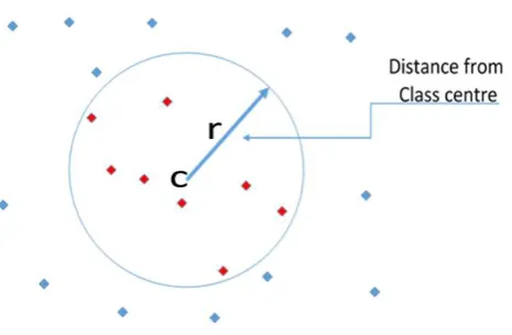
Figure 1. Filtering data samples in the proposed algorithm. Red rhomboids inside the circle centred at cluster head c will not be fed into the SVM training module.

To combine k-means and SVM, we first train k-means as explained above using the entire training

dataset. As a result, k classes, each corresponding to one appliance, are formed with a centroid as

head. Next, all feature vectors falling in Classi that are at an Euclidean distance larger than r from

their head, form a subset of feature vectors Ci that is removed from Class i and used to train an

SVM for Appliance i. r is a pre-set threshold, unique for each house, obtained heuristically, that is

used to trade offcomplexity and performance. See Fig. 1 for an illustration. Note that, in this way,

SVM will be trained using a significantly reduced dataset obtained from the trained k-means classifier,

and hence the combined k-means+SVM complexity will be reduced, compared to SVM classification

alone. Algorithm 1 shows the training steps, whered(x,y) denotes the Euclidean distance between

vectorsxandy.

Algorithm 1Training: Perform training on the extracted features of the collected dataset.

functionTrain(Labelled training datasetL,|M|,r)

k=|M| .Number of Appliances

[Cluster,c]=kmeans(k,L) .Call kmeans function

.ReturnsClusterdistribution and cluster headsc.

fori=1 :kdo

Ci={∅}

for∀l∈Clusterido .Clusteridenotesi-th cluster inCluster

ifd(l,ci)≥rthen .cidenotesi-th element ofk-length vectorc

Ci=CiS_{

l}

end if end for

S V MT rain(Ci) .Call conventional SVM training function

end for end function

Algorithm 2Testing: Perform testing on the extracted features of the collected dataset.

functionTest(Testing dataset,Clusters,c,|M|,r)

k=|M| .Number of Appliances

fori=1 :kdo

Ci={∅}

for∀l∈Clusterido

ifd(l,ci)≥rthen

Ci=CiS_{

l}

elseClassify sampleito the appliance corresponding toci

end if end for

S V MT est(Ci) .Call conventional SVM testing function

end for end function

maintains high performance, since SVM improves classification for samples that would most likely be incorrectly classified using the trained k-means.

Testing is straightforward and shown in Algorithm 2. Samples at distance less thanrfrom a cluster

head are classified to the appliance corresponding to that cluster head. All other samples are classified using SVM.

3.2. Database of appliance signatures

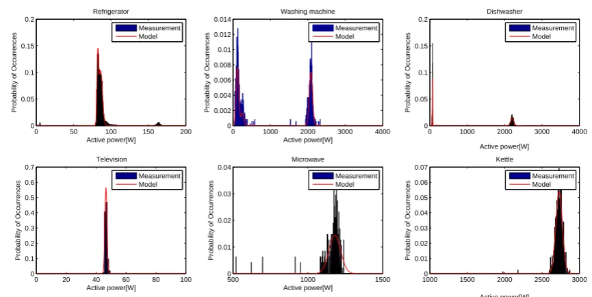
All domestic appliances are designed to work within a certain active power range, which can often be found in the appliance instruction manual. However, in practice, the actual active power measured will deviate due to electrical noise, interference, ageing, etc. The probability density function (PDF) of active power captures the electrical behaviour of an appliance, e.g., Figures 2 and 3 show the pdf for several domestic appliances in the REFIT and GREEND datasets. Due to the typical low sampling rates

(≤ 1 Hz) expected of smart meters, we focus only on steady state operation, automatically removing

transient values from each appliance operation during data cleaning. As shown in Figures 2 and 3, the active power follows a Gaussian mixture distribution. See Subsection 4.4, which validates Gaussian modelling using root-mean squared error (RMSE) with respect to the true power load curve obtained through sub-metering.

0 50 100 150 200 0 0.05 0.1 0.15 0.2 Active power[W]

Probability of Occurrences

Refrigerator

Measurement Model

0 1000 2000 3000 4000 0 0.002 0.004 0.006 0.008 0.01 0.012 0.014 Active power[W]

Probability of Occurrences

Washing machine

Measurement Model

0 1000 2000 3000 4000 0 0.05 0.1 0.15 0.2 Active power[W]

Probability of Occurrences

Dishwasher

Measurement Model

0 20 40 60 80 100 0 0.1 0.2 0.3 0.4 0.5 0.6 0.7 Active power[W]

Probability of Occurrences

Television

Measurement Model

500 1000 1500 0 0.01 0.02 0.03 0.04 Active power[W]

Probability of Occurrences

Microwave

Measurement Model

10000 1500 2000 2500 3000 0.01 0.02 0.03 0.04 0.05 0.06 0.07 Active power[W]

Probability of Occurrences

Kettle

Measurement Model

Figure 2. Probability density distribution of six REFIT dataset appliances, charac-terised by Gaussian mixture distribution. Fitted data shows appliance power sampled at 8 sec for five households over a period of 5 weeks.

Hi-Fi, PCs. Each database entry comprises the duty cycle for each appliance at the dataset’s original sampling rate. Additionally, just like [11], each appliance’s power load profile is modelled using a Gaussian mixture model, obtained via curve fitting. The model is represented in the database by its

mean, variance, PDF and the first two correlation coefficients, calculated as:

R(τ)=

P

t(Xt−µ)(Xt+τ−µ)

σ2 , (1)

whereXt is active power measurement at time instancet,µis the mean power value,σ2is the variance

andτis the sample lag.

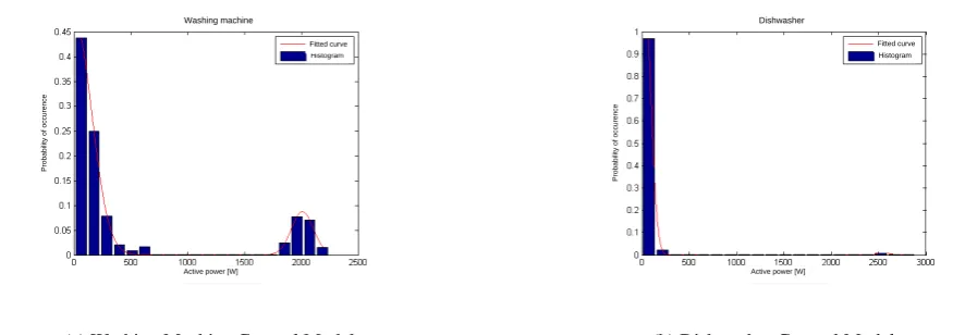
We aim to build one general model for each type of appliance, i.e., one generic refrigerator model that would best fit all refrigerator makes and models encountered in our dataset houses. While this kind of generalization may not work for some appliances like televisions, all monitored washing machines

and dishwashers have similar signatures. Figure 4 shows Gaussian distribution models for different

Televisions (TVs). It is obvious from the figure that energy consumptions of different TV makes and

models are very different. Figures 5a and 5b show the Gaussian distribution model for the washing

machine and dishwasher obtained using the data from all GREEND houses. It can be seen that an

efficient general model can be formed that represents well different appliance brands, which is due to

the fact that all tested washing machines and dishwashers in our dataset have signatures that are similar, in the sense that there are clearly identifiable cycles, each with a similar operational power range.

Some appliances, referred to as multi-state appliances, such as washing machine or dishwasher,

Probability of occurence

Fitted curve Histogram Coffee machine

Active power [W]

Probability of occurence

Fitted curve Histogram Radio

Active power [W]

Probability of occurence

Fitted curve Histogram Hair dryer

Active power [W]

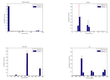
Figure 3. Probability density function for four different appliances from the GREEND dataset. Histograms are showing true data obtained via sub-metering.

3.3. Approach 2 using house-agnostic training data

Using the appliance active power signatures from the database, a general appliance model is gen-erated for each appliance type, using the PDF of this appliance type. Note that the appliance PDF is

generated from the active power signatures of that appliance, obtained from different makes and

mod-els in different houses in our datasets. This way, we generate onegeneralGaussian mixture model for

each appliance type (e.g., washing machine, kettle, etc.), described by its mean and variance.

Based on the generated model, we design two methods. The first method draws samples from

the obtained Gaussian mixture distribution that are used to form a training dataset. Effectively, the

labelled dataset, in the case of Approach 1, that needs to be obtained via time-diary or sub-metering, is replaced by data samples generated from the Gaussian distribution for that particular appliance. Then, Algorithm 1 can readily be used to perform labelling, without any need for a time diary or sub-metering. The testing approach is the same as in the supervised method above.

The second proposed method, called Mean-variance General Model approach, uses only mean and variance of the generated general Gaussian mixture model. That is, unlike the previous approach, this approach does not draw samples from the model, which in turn implies that no other features (such as those shown in Table 1) can be used, besides mean and variance for classification of k-means and SVM. Due to its limited feature space, this approach is not expected to perform well, due to statistical similarities of appliance signatures.

Note that both approaches can be used with different event-based supervised methods. That is, the

Probability of occurence

Active power [W] Kitchen TV

Fitted curve Histogram

Probability of occurence

Living room TV

Active power [W]

Fitted curve Histogram

Probability of occurence

Active power [W] LCD TV

Histogram Fitted curve

Probability of occurence

Active power [W]

Histogram Plasma TV

Fitted curve

Figure 4. Different distributions of different TV types from the GREEND dataset. His-tograms are showing true data obtained via sub-metering.

training-based approaches next.

4. Results and Discussion

In this section we present our experimental results and discuss our main findings. We use the pub-licly available REDD dataset [23] and GREEND dataset [24] with 1min and 1sec resolution, respec-tively, as well as our measurements that constitutes the REFIT dataset [7] acquired at 8sec resolution. The training size varied in the experiments, but testing is always performed on four weeks worth of data. We used Spring, Summer and Autumn periods for training and testing.

We organize the results as follows. First, the performance of the proposed Approach 1 with house-specific training, with respect to k-means and SVM approaches separately, is assessed. We show that combining k-means and SVM, as proposed in the previous section, leads to significant reduction in processing time while providing similar accuracy to that of SVM-based disaggregation. Then, we

dis-cuss feature selection and show that different classification features are suitable for different appliances.

Hence, we propose that the choice of feature(s) to use for each appliance is made during training. The third set of results assesses accuracy of the proposed approach when the training period varies and labelling errors occur. We show that the proposed approach is not sensitive to the size of the training period and presence of labelling errors. We use HMM-based [12], k-means-based, and the SVM-based approach as benchmarks.

Probability of occurence

Washing machine

Active power [W]

Histogram Fitted curve

(a) Washing Machine General Model

Probability of occurence

Dishwasher

Active power [W]

Histogram Fitted curve

(b) Dishwasher General Model

Figure 5. Washing machine and dishwasher general models.

provides close performance to the approach using house-specific training data, but without the require-ment for training on the specific house data.

4.1. Performance metrics

The evaluation metrics used are precision (PR), recall (RE) and F-Measure (FM), commonly used

in NALM literature ([8, 17]) and defined as:

PR= T P/(T P+FP) (2)

RE =T P/(T P+FN) (3)

FM = 2∗(PR∗RE)/(PR+RE), (4)

where true positive (TP) presents the correctly detected event, false positive (FP) represents an incorrect detection, and false negative (FN) indicates that the appliance used was not identified.

4.2. Comparison with k-means and SVM

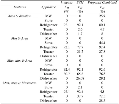
First, we evaluate the improvement obtained by combining k-means and SVM into a combined ap-proach. Tables 1 and 2 show results obtained using House 2 from the REDD dataset (see the conference version [18] for other results) for the trained k-means-based, SVM-based, and the combined algorithm. All three algorithms always use the same edge detection and feature extraction method explained in the previous section.

Table 1. Comparison between the three methods usingFM for REDD data House 2.

k-means SVM Proposed Combined

Features Appliance FM FM FM

(%) (%) (%)

Area&duration MW 0 0 25.9

Stove 0 0 0

Refrigerator 92.1 92.1 80.1

Toaster 0 2.6 4.7

Dishwasher 0 1.7 8

Min&Area MW 0 0 0

Stove 0 0 44.4

Refrigerator 92.1 72.7 92.4

Toaster 0 31.7 27.8

Dishwasher 0 0 0

Max, dur.&Area MW 0 0 0

Stove 0 0 0

Refrigerator 92.4 92.1 92.6

Toaster 30.7 65.8 76.5

Dishwasher 0 26.08 29.2

Max, area&Max/mean MW 0 0 0

Stove 0 2.1 0

Refrigerator 92.1 92.4 93

Toaster 0 37.7 72.5

Dishwasher 0 0 28.5

Table 2. Comparison between the three methods using Execution time (training and testing) for REDD data House 2.

k-means SVM Proposed Combined

Features train test train test train test

(sec) (sec) (sec) (sec) (sec) (sec)

Area&duration 0.27 0.27 1.5 0.91 0.38 0.69

Min&Area 0.24 0.29 1.19 0.72 0.15 0.53

Max, dur. &Area 0.29 0.23 1.15 0.88 0.16 0.71

We tested different two-, three-, four, and five-dimensional classifiers by extracting different fea-tures (event window area, time duration, minimum or maximum power value in the event window or maximum-to-mean value ratio) and present results for the best two two-dimensional and two three-dimensional classifiers.

Marked with bold typeface are the better performing features for each appliance. One can see

that for different appliances different features give the best performance. For example, onlyArea and

Duration classification returns a non-zero disaggregation accuracy for the microwave. Since we are

classifying one appliance at a time, it is possible to adapt classification features from appliance to appliance. Thus, during training, the best features to use are identified per appliance which are then used during testing. In the following, we refer to this method, as the proposed combined method.

It can be seen from the tables that the SVM-based method outperforms the trained k-means, except for the refrigerator, but requires more time for both training and testing. For example, the best SVM-based NALM result for the toaster is obtained for the 3D classifier using maximum, duration and area is 2.5 times more accurate than the best k-means-based performance, but is over 3 times slower when performing training and testing.

The combined approach clearly outperforms both the k-means and SVM-based approaches for all appliances, through the appropriate selection of features for every appliance. While execution time for k-means is the smallest as expected, the combined approach executes faster than the SVM-based approach, confirming that combining both k-means and SVM approaches reduces the SVM execution time. Indeed, the proposed method reduces the operation time of SVM by reducing the number of samples fed to the SVM classifier, through clustering.

KmeansSVM Proposed Refrigerator Stove MW Toaster DishW 0 500 1000 TP

Number of Occurrences

KmeansSVM Proposed Refrigerator Stove MW Toaster DishW 0 100 200 FP

Number of Occurrences

KmeansSVM Proposed Refrigerator Stove MW Toaster DishW 0 20 40 60 FN

Number of Occurrences

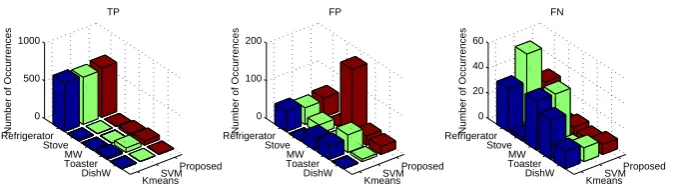
Figure 6. TP, FP, and FN for each appliance, after disaggregation by k-means, SVM and the proposed combined method for House 2 in the REDD dataset. MW =microwave, DishW=Dishwasher.

The performance of the three approaches can be explained by looking at Figure 6 which shows TP, FP, and FN values for the three approaches for all five appliances. The proposed, combined approach has the largest number of TPs and lowest number of FNs. k-means approach has generally low FP,

but high FN and low TP. For example, for the microwave k-means and SVM yields TP= 0, FP=32

and 0, respectively, and FN= 39. On the other hand, the proposed approach detects instances of the

Figure 7. FM for the four methods for three REDD houses and three different training

set sizes.

detected almost all occurrences of microwave, but had too high sensitivity detecting the microwave

running when it was not, due to very short microwave’s duty cycle. This reduced the overall FM for

House 2 as shown in Table 8.

4.3. Accuracy and Complexity

First, we test accuracy of the algorithms when the training time varies. Intuitively, by increasing the training time, the performance should improve, since more samples will be available to train classifiers. However, longer training time increases complexity and burden on customers if time diaries are used. That is why, it is desirable to have methods that do not require long training periods.

Figure 7 shows the average results for three REDD houses, benchmarked against the following three methods: the trained k-means based approach, the SVM-based approach and the HMM-based method of [12]. All methods used the same period for training and testing. K-means, SVM, and the proposed method use the optimal features (see Table 2).

FM results are given for 3 different training sizes, namely 2000 (roughly 2 days), 5000 (roughly 5

days), and 7000 samples (roughly one week). Testing is done using four-week worth of data.

It can be seen that the proposed combined method either outperforms HMM-based and SVM-based approaches or provides a similar accuracy. k-means based approach provides lower disaggregation

accuracy. Relatively high FM obtained by k-means is somewhat misleading and can be explained by

low FP values, despite low TP and high FN values (see Figure 6). On the other hand, high FP value for

microwave, reduced overallFMfor the proposed method.

slightly better performance for smaller training sets due to better quality of the training data. In average over all three houses, the proposed method outperforms all other approaches for training sizes of 2000

and 7000 and is the second-best method for the training size of 5000 after k-means, whoseFMis not a

true reflection of the performance (see Figure 6).

Table 8, in the appendix, shows the execution time which includes time spent on training and testing. The training execution time of the proposed method slightly increases as the training set size increases but it is still significantly lower than that of the HMM-based approach for all houses and all training sizes. Indeed, the proposed method needs roughly 18 and 3.5 times less time for testing than HMM and SVM, respectively, and 13 and 2.5 times less time for training than HMM and SVM, respectively. In average over all three houses, the proposed method is 2.75 times and 2 times faster for training and testing, respectively, than the SVM method and over 90 and 50 times faster, for training and testing, respectively, than the HMM-based method.

Table 3. FM results for House 2 obtained by introducing errors in the labelled dataset

used for training.

Error rate Refrigerator Toaster Dishwasher

0 % 93.6 46.7 0

K-means 5 % 91.9 57.4 0

15 % 91.8 2.4 0

20 % 91.9 2.4 0

0 % 92.5 69.13 26

SVM 5 % 92.2 43.6 44.4

15 % 92 45.3 0

20 % 91.7 0 0

0 % 94.3 79.1 29.2

Proposed 5 % 91.8 11.4 17.39

15 % 93.3 11.9 42.8

20 % 91.9 8.9 45.3

0% 87.69 64.9 12.32

HMM 5 % 83.42 64.9 12.32

15 % 83.42 49.97 12.32

20% 83.55 46.97 12.32

Table 3 shows the accuracy of the approaches when labelling errors occur as FM vs the error rate

for three different appliances. The error rate is the percentage of wrongly labelled data during training.

Note that the proposed method is fairly not sensitive to the labelling errors except for the toaster whose operation is very short and easily confused with other appliances.

4.4. Modelling Validation

In this section, we validate the proposed Gaussian mixture mathematical model for the pdf of active power for domestic appliances as described in Section 3.

Table 4. RMSE, mean [W], variance, 1st order correlation coefficient and2nd order correlation coefficient for different TV’s in Houses 4 and 5 from GREEND dataset. GM denotes the general model obtained by considering data from all GREEND houses.

Appliance Mean value Variance RMSE 1st Cor. 2nd Cor.

House4 Kitchen TV 42.14 2.88 5.68 E-2 0.2698 0.2455

House4 living room TV 16.68 48.41 4.9 E-3 0.0962 0.0184

House5 LCD TV 35.25 2.46 3.77 E-4 0.0199 0.0768

56.24 1.07

House5 Plasma TV 144.47 13.94 8.3 E-3 0.1442 0.0746

201.45 34.67

GM TV 28.5 4.117 0.0169

55.98 6.047

190.8 72.37

Refrigerator Fridge−Freezer Oven Hood Washing machineDishwasher TV Microwave Toaster Stereo player Kettle Oven head fan Aggregate 10−7

10−6

10−5 10−4 10−3 10−2 10−1

100

101

Appliances

RMSE

Gaussian Laplace Log−normal

Figure 8. RMSE of Gaussian, Laplace and Log-normal models for 13 appliances from REFIT and GREEND datasets, and the REFIT aggregate meter reading, all shown on a log-scale.

by averaging in time and across different houses. It can be seen that the Gaussian mixture model

is the best fit for all appliances, especially for high loads such as kettle and toaster. As expected, the Gaussian mixture model is also the best for the aggregate readings, since it is a sum for nearly independent processes. This validates our approach of using the Gaussian mixture model (red line in Figure 2) to build the distribution model of all appliances. We also note that RMSE is insignificantly small except for low-consumers such as TV and Stereo Player. These findings are similar to those reported in [11].

of this are that drawing on the general model for TV for training the unsupervised method would not result in high accuracy. A supervised approach trained on that household’s dataset would be more

effective in the case of TV.

Table 5. RMSE, mean [W], variance, 1st order correlation coefficient and 2nd or-der correlation coefficient for different washing machines and dishwashers of different GREEND houses. GM denotes the general model obtained by considering data from all GREEND houses.

Appliance Mean value Variance RMSE 1st Cor. 2nd Cor.

H0 WM 80.1 93.8 4.2 E-3 0.0751 -0.1059

1955.6 73.07

H1 WM 40.4 73.97 3.8 E-3 0.022 -0.1126

1991.7 90.92

H3 WM 94.7 115.59 1.91 E-2 0.0609 -0.0838

1957.8 69.51

H4 WM 54.9 93.71 3.3 E-3 0.0298 -0.2105

597.4 13.77

1946.1 224

GM WM 139.2 119.93 3.2 E-3

2009.3 90.45

H0 DW 77 14.05 6.17 E-5 0.1925 0.1226

1953.3 77.8

H1 DW 13.7 28.9 4.5 E-5 -0.042 -0.1111

1796 29.54

H2 DW 18.1 33.19 9.97 E-5 -0.066 -0.1186

2071.3 38.79

GM DW 48 42.56 6.7 E-3

2480 368.2

Table 5 confirms that the RMSE obtained using the general model averaging appliance data from all the houses, is still small across all GREEND houses.

4.5. Approach based on house agnostic training data

Tables 6 and 7 show, for two appliances, the relative performance of the following methods: Ap-proach 1 - Regular training using house-specific training data which uses real labelled data from the specific house for training; Approach 2 - disaggregation using house-agnostic training data that uses features derived from the Gaussian distribution models and draws samples from the Gaussian distri-bution to train the k-means and SVM, and finally, the mean-variance approach using the mean and variance features directly from our Gaussian General model directly from our databases, called Gen-eral Model (GM). As benchmarks, we used HMM-based and SVM-based methods. The models were

built using at least three houses from the GREEND dataset and tested using two different houses. We

Tables 6 and 7 show that the proposed approach using house-agnostic training data shows compet-itive performance to that of disaggregation using house-specific training data. The GM method could not detect washing machine events with only mean and variance as features, whereas the approach

using house-agnostic training data used 2D classifiers with different features such as maximum load

value, area and duration. The reason for this is that mean and variance of dishwashers in our dataset are very fairly standard, which is not the case with washing machines. Hence, we can conclude that it is necessary to train the disaggregation methods, drawing samples from the database, rather than using the features directly for the classification.

Table 6. Results of washing machine disaggregation in GREEND House 1 (H1) and House 2 (H2), using three different methods. Houses 3, 4 and 5 are used for training.

House-specific training House-agnostic training GM

H % SVM Combined HMM SVM Combined SVM Combined

PR 63.88 100 0.5 78.57 72.54 0 0

H1 RE 100 65.21 95.5 71.73 80.43 0 0

FM 77.96 78.94 1.04 75.00 76.28 0 0

PR 83.33 87.50 2.14 83.33 88.23 6.26 9.09

H2 RE 100 93.33 96.4 100 100 3.33 3.33

FM 90.90 90.32 4.19 90.90 93.75 4.34 4.87

Table 7. Results of dishwasher disaggregation in GREEND House 2 (H2) and House 3 (H3), using three different methods. Houses 1, 4 and 5 are used for training.

House-specific training House-agnostic training GM

H % SVM Combined HMM SVM Combined SVM Combined

PR 97.01 97.01 24.68 92.06 88.40 92.29 94.20

H2 RE 100 100 3.19 89.23 93.84 100 100

FM 98.48 98.48 5.66 90.62 91.04 96.29 97.01

PR 87.50 87.50 2.51 87.50 87.50 83.33 83.33

H3 RE 100 100 82 100 100 71.42 71.42

FM 93.33 93.33 4.88 93.33 93.33 76.92 76.92

5. Conclusion

Our study provides the opportunity to make a trade-offbetween accuracy and complexity or execu-tion time. Generally what we observed is that the time savings far outweigh the accuracy. The next steps are further development of the database of signatures based on crowdsourcing and testing the

proposed methods using different datasets.

Acknowledgments

This work is supported in part by the UK Engineering and Physical Sciences Research Council

(EPSRC) projects REFIT EP/K002368, under the Transforming Energy Demand in Buildings through

Digital Innovation (BuildTEDDI) funding programme.

Conflict of interest

No conflict of interest. All authors contributed to paper writing, data analysis and algorithm design. Hana Altrabalsi implemented the proposed algorithms, ran simulations and generated the results.

References

1. Smart metering equipment technical specifications: Second version: Part 2.Department of Energy

&Climate Change UK, Dec. 2013.

2. Armel KC, Gupta A, Shrimali G, et al. (2013) Is disaggregation the holy grail of energy efficiency?

The case of electricity.Energy Policy52: 213–234.

3. Hart G, Nonintrusive Appliance Load Data Acquisition Method,MIT Energy Laboratory

Techni-cal Report, Sept. 1984.

4. Zeifman M, Roth K (2011) Nonintrusive appliance load monitoring: Review and outlook. IEEE

Trans Consumer Electronics57: 76–84.

5. Zoha A, Gluhak A, Imran MA, et al. (2012) Non-intrusive load monitoring approaches for

disag-gregated energy sensing: A survey.Sensors12: 16838–16866.

6. Perez KX, Cole WJ, Baldea M, et al. (2014) Meters to models: Using smart meter data to predict

home energy use. in Process. ACEEE Summer Study on Energy Efficiency in Buildings, Pacific

Grove, CA.

7. Murray D, Liao J, Stankovic L, et al., A data management platform for personalised real-time

energy feedback. inProc EEDAL-2015 8th Int Conf Energy Efficiency in Domestic Appliances

and Lighting,Lucerne-Horw, Switzerland, Aug. 2015.

8. Liao J, Elafoudi G, Stankovic L, et al. Power disaggregation for low-sampling rate data.2nd Int.

Non-intrusive Appliance Load Monitoring Workshop,Austin, TX, June 2014.

9. Marchiori A, Hakkarinen D, Han Q, et al. (2011) Circuit-level load monitoring for household

energy management,IEEE Pervas Comput10: 40-48.

10. Berges M, Goldman E, Matthews HS, et al. (2011) User-centered non-intrusive electricity load

11. Kim H, Marwah M, Arlitt M, et al., Unsupervised disaggregation of low frequency power

mea-surements, inProc 11th SIAM Int Conf Data Mining,Mesa, AZ, April 2011.

12. Parson O, Ghosh S, Weal M, et al. (2012) Non-intrusive load monitoring using prior models of

general appliance types. inProc. the 26th Conf. Artificial Intelligence (AAAI-12), Toronto, CA,

pp. 356–362.

13. Kolter J, Jaakkola T (2012) Approximate inference in additive factorial HMMs with application

to energy disaggregation. inJ Machine Learning22: 1472–1482.

14. Johnson MJ, Willsky AS (2013) Bayesian nonparametric Hidden Semi-Markov Models. J

Ma-chine Learning Research14: 673–701.

15. Kolter J, Batra S, Ng AY, Energy Disaggregation via Discriminative Sparse Coding. in Proc

Advances in Neural Inform Processing Sys 23 (NIPS 2010).

16. Shao H, Marwah M, Ramakrishnan NA, Temporal motif mining approach to unsupervised energy

disaggregation. in Proc. the 1st Int Workshop Non-Intrusive Load Monitoring, Pittsburgh, PA,

May 2012.

17. Elafoudi G, Stankovic L, Stankovic V, Power disaggregation of domestic smart meter readings

using Dynamic Time Warping. ISCCSP-2014 IEEE Intl Symp Communications, Control, and

Signal Processing,Athens, Greece, May 2014.

18. Altrabalsi H, Liao J, Stankovic L, et al., A low-complexity energy disaggregation method:

Perfor-mance and robustness.SSCI-2014 IEEE Symp Comput Intelligence Applications in Smart Grid,

Orlando, FL, Dec. 2014.

19. Xia XL, Lyu MR, Lok LM,et al., Methods of decreasing the number of support vectors via k-mean

clustering.in Proc ICIC 2005, LNCS 3644, pp. 717–726, Spinger-Verlag Berlin Heidelberg, 2005.

20. Wang j, Wu x, Zhang C (2005) Support vector machines based on K-means clustering for

real-time business intelligence systems.Int J Business Intelligence and Data Mining1: 54–64.

21. Yao Y, Liu Y, Yu Y, et al. (2013) K-SVM: An effective SVM algorithm based on k-means

cluster-ing.J Computers 8: 2632–2639.

22. Gu Q, Jan J, Clustered Support Vector Machines. in Proc AISTATS-2013 16th Int Conf Artificial

Intelligence and Statistics,Scottsdale, AZ, 2013.

23. Kolter J, Johnson M. REDD: A public data set for energy disaggregation research. inWorkshop

on Data Mining Applications in Sustainability (SIGKDD), San Diego, CA, 2011.

24. Monacchi A, Egarter D, Elmenreich W, et al. GREEND: An Energy Consumption Dataset of

Households in Italy and Austria.in Proc IEEE SmartGridComm, Venice, Italy, Nov. 2014.

25. Gao J, Giri S, Kara EC, et al. ( 2014) PLAID: a public dataset of high-resolution electrical

appli-ance measurements for load identification research: demo abstract.in Proc the 1st ACM

Confer-ence on Embedded Systems for Energy-Efficient Buildings, 198-199.

26. Ruzzelli AG, Nicolas C, Schoofs A, et al. (2010) Real-time recognition and profiling of appliances

through a single electricity sensor.in Proc IEEE SECON-2010 7th Annual Conf Sensor Mesh and

Ad Hoc Communications and Networks, 1–9.

27. Laughman C, Lee K,Cox R, et al. (2003) Power signature analysis. IEEE Power and Energy

28. Liang J, Ng SKK, Kendall G, et al. (2010) Load signature study part I: Basic concept, structure,

and methodology.IEEE Trans Power Delivery25: 551–560.

29. Berges M, Goldman E, Matthews HS, et al., Learning systems for electric consumption of

build-ings. inProc 2009 ASCE Int Workshop Computing in Civil Engineering, Austin, TX, 2009.

30. Barker s, Kalra s, Irwin D, et al., NILM redux: The case for emphasizing applications over

accuracy.NILM-2014 Workshop,Austin, TX, June 2014.

31. Markonin S, Bajic IV, Popowich F, Efficient sparse metric processing for nonintrusive load

mon-itoring.2nd Int Non-intrusive Appliance Load Monitoring Workshop,Austin, TX, June 2014.

32. Al-Harbi SH, Rayward-Smith VJ (2006) Adapting k-means for supervised clustering. Appl

In-tell24: 219–226.

Appendix

Table 8. F-measure [%] and Execution time for training and testing [sec] for the three REDD houses (H) using three different training sizes (t. size) given in number of sam-ples.

HMM k-means SVM Proposed

H t. size train test FM train test FM train test FM train test FM

2000 15.18 21.29 73.53 0.18 0.18 71.9 0.37 0.57 73.8 0.19 0.32 73.2

1 5000 23.79 19.27 75.58 0.25 0.25 71.2 0.76 0.65 74.2 0.27 0.25 71.7

7000 28.32 22.90 77.06 0.2 0.2 73 0.83 0.78 80.37 0.7 0.26 77.52

2000 18.38 18.56 81.03 0.09 0.25 89.69 0.43 0.72 85.9 0.1 0.32 84.7

2 5000 21.13 18.03 82.38 0.06 0.2 84.6 0.84 0.72 87.1 0.3 0.34 84.4

7000 22.77 18.09 82.38 0.23 0.23 84.7 1.15 0.79 85.5 0.25 0.55 82.17

2000 20.52 10.99 69.92 0.07 0.18 86.5 0.33 0.35 83.1 0.12 0.2 96.58

6 5000 22.46 13.91 72.76 0.09 0.14 96.58 0.56 0.45 81.5 0.15 0.26 88

7000 30.22 16.19 72.76 0.24 0.24 97 0.69 0.53 80.6 0.11 0.28 95.58

c

2016, Jing Liao, et al., licensee AIMS Press.

This is an open access article distributed under the terms of the Creative Commons Attribution License