Electrothermal flows generated by alternating and rotating electric fields in microsystems

doi:10.1017/S0022112006001595 Printed in the United Kingdom

Electrothermal flows generated by alternating

and rotating electric fields in microsystems

By A. G O N Z ´A L E Z1, A. R A M O S2†, H. M O R G A N3, N. G. G R E E N3 A N D A. C A S T E L L A N O S2

1_{Departamento F´ısica Aplicada III, E.S.I. University of Seville, Camino de los Descubrimientos}

s/n, 41092 Sevilla, Spain

2_{Departamento Electr ´onica y Electromagnetismo, University of Seville, Avda. Reina Mercedes}

s/n, 41012 Sevilla, Spain

3_{School of Electronics and Computer Science, University of Southampton, SO17 1BJ, UK}

(Received27 May 2005 and in revised form 2 March 2006)

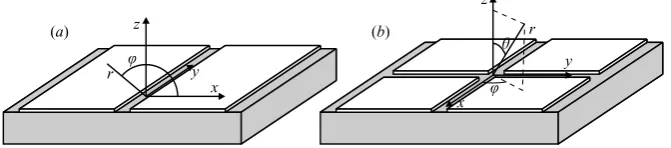
Electrothermal motion in an aqueous solution arises from the action of an electric field on inhomogeneities in the liquid induced by temperature gradients. The temperature field can be produced by the applied electric field through Joule heating, or caused by external sources, such as strong illumination. Electrothermal flows in microsystems are usually observed at applied signal frequencies around 1 MHz and voltages around 10 V. In this work, we present self-similar solutions for the motion of an aqueous solution in a constant temperature gradient placed on top of: (a) two coplanar electrodes subjected to an a.c. potential difference, and (b) four coplanar electrodes subjected to a four-phase a.c. signal, generating a rotating field. The first case produces two-dimensional rolls whereas the second case produces a liquid whirl. Finally, we present experimental results of electrothermal liquid flows generated by alternating and rotating electric fields under strong illumination, and these experiments are compared to the analytical solutions. The induced rotating flow could be used in the mixing ofanalytes and of liquids in microsystems.

1. Introduction

In microsystems, a.c. electric fields can interact with a liquid through several mechanisms (Castellanoset al.2003), ranging from bulk effects such as electrothermal effects and natural convection (M¨uller et al. 1993; Arnold 2001) to surface effects such as ac electro-osmosis (Ramos et al.1999; Ajdari 2000; Bazant & Squires 2004). Flows driven by electrothermal forces are often present in the dielectrophoretic manipulation of colloidal particles in microsystems (M¨uller et al. 1996; Ramos et al. 1998; Green et al. 2000, 2001). Electrothermal fluid flow is due to the action of an electric field on thermally induced gradients of conductivity and permittivity in the fluid (Melcher & Firebaugh 1967; Melcher 1981). The gradients of temperature can be produced by external sources, such as strong illumination (Green et al. 2000), or caused by the applied electric field through Joule heating (M¨uller et al.1993; Gimsa, Eppmann & Pr¨uger 1997; Wang, Sigurdson & Meinhart 2005). Observations and estimates show that electrothermal effects are important in microsystems for frequencies of the order of 1 MHz and voltages of the order

r

x y z

θ r

x

y z

(a) (b)

Figure 1.Diagrams showing the coordinate systems for: (a) the two coplanar electrodes and

(b) the four coplanar electrodes.

of 10 V (Green et al. 2001; Castellanos et al. 2003). These frequencies are much greater than typical frequencies of electrode polarization. For these frequencies, electrokinetic flows such as a.c. electro-osmosis are almost certainly negligible since the charges have no time to accumulate in the diffuse double layer (Ramos et al. 1999). In this work, we will consider that the applied signals have frequencies in this regime, i.e. ω1/RbCDL, where Rb is the resistance of the bulk electrolyte

between electrodes and CDL the capacitance of the electrode/electrolyte double

layer.

In this paper, we present some self-similar solutions for the fluid flow induced by a combination of electric fields and externally imposed gradients of temperature in microelectrode structures. First, we consider the two-dimensional motion of an aqueous solution placed on top of two coplanar, parallel electrodes subjected to an a.c. potential difference when there is either a vertical or a horizontal gradient of temperature. This geometry is shown in figure 1(a). Self-similar solutions for the electric field and liquid motion are obtained. These solutions are relevant to some fluid flows observed under strong illumination (Greenet al.2000).

Secondly, we study the three-dimensional problem of an aqueous solution lying on four coplanar electrodes placed in each quadrant (see figure 1b). The electrodes are driven by a four-phase a.c. signal and this generates a rotating electric field. Previously studied two-dimensional configurations are used to solve the electrical three-dimensional problem analytically. Then, the solution for the liquid flow is obtained and it is shown that this produces a rotation of the liquid. Such a system could be used in the design of rotatory micro-pumps and for local mixing in microfluidics. Also, these results are relevant to electrorotation experiments when combined with laser tweezers, where electrothermal flow rotation has been observed (Schnelleet al. 2000).

2. Formulation of the problem

The mathematical problem involves a coupled system of electrical, mechanical and thermodynamical equations. The electric field moves the liquid, and this motion in turn convects charge and heat. Nevertheless, the low velocities involved in microsystems mean that these convection terms can be neglected, and therefore, the electrical and thermodynamical problems can be solved independently with the solution then inserted into the mechanical problem (Ramos et al.1998).

To determine whether the temperature field is independent of the velocity field, the P´eclet number must be calculated, given byvl/κ (v, typical velocity;l, typical system length; κ, thermal diffusivity). The P´eclet number for microsystems is typically very small, showing that heat convection is small compared to heat diffusion (Castellanos et al. 2003).

In the bulk electrolyte, the electrical current j is given very approximately by Ohm’s law, j=σE (Levich 1962). For a binary monovalent electrolyte at rest, the current density can be expressed as

j =e(n+µ++n−µ−)E−e(D+∇n+−D−∇n−)−e(D+Tn+−D₋Tn−)∇T , (1)

with e the absolute value of electronic charge, µ, D, DT_{, n}

+ and n−, the mo-bility, diffusion coefficient, thermodiffusion coefficient and number densities of positive and negative ions. For typical electric fields of interest in microsystems, the electro-migration current dominates. In effect, the ratio between diffusion and electrical drift is of the order of D+/µ+El=kBT /eEl (Chen et al. 2005), and the ratio

between thermodiffusion and electrical drift is of the order of T DT

+/µ+El∼ T D+/T µ+El=kBT /eEl (Putnam & Cahill 2005). Both ratios are much less

than one (kBT /e≈0.025 V, El∼5 V). Here kB is Boltzmann’s constant, T is the

absolute temperature andl is a typical distance. In addition, Gauss’ law suggests that the liquid bulk is quasi-electroneutral on the micrometre length scale. The relative difference in ion number densities (n+−n−)/n+=∇ ·(εE)/en+ is of the order of the parameter Λ=εE/eln+ (Saville 1997; Castellanos et al. 2003), which is very small for typical values in microsystems. The conductivity in Ohm’s law is then given by σ=e(µ++µ−)n0, with n0 the unperturbed ion density.

In this work, we assume that the origin of conductivity gradients is due to the fact that ionic mobilities depend on temperature. The conductivity is then a given function of temperature σ=σ(T). We do not take into consideration gradients of concentration, as in Chen et al. (2005). Gradients of concentration can appear at the electrodes owing to concentration polarization. For applied a.c. voltages of high enough frequencies (ω1/RbCDL), negligible charge is accumulated at the double

layer and no concentration polarization is expected. This ‘RC time’ of a bulk resistor in series with a double-layer capacitor is of the order of (ε/σ)(l/λD), whereλD is the

Debye length (Ramos et al.1999; Bazant et al. 2004). We consider a.c. signals with angular frequencies that are ωσλD/εl (f =ω/2π1 kHz forσ∼10−3 S m−1 and l∼10−5_{m). In addition, the diffusion equation that governs the conductivity (Bazant} et al. 2004; Chenet al. 2005) gives a typical diffusion length of the order of √D/ω, which is very small, of the order of the Debye length for frequencies around σ/ε. Therefore, we do not expect gradients of concentration in the bulk.

imposed temperature fields in Green et al. (2001); Castellanos et al. (2003). It was shown that for applied voltages smaller than or equal to 10 V, and conductivities less than 0.03 S m−1_{,Joule heating is insufficient to generate the gradients of temperature} that account for observed flow velocities (which are of the order of 50µm s−1_{). Wang} et al. (2005) have measured fluid velocities around 100µm s−1 _{for electrothermal} flow induced by Joule heating at voltage amplitudes of 10–15 V, but in a fluid of conductivity σ= 0.056 S m−1_{. For the conductivity we analyse in the experimental} section, the same voltages would generate fluid velocities around 5µm s−1 _{or less.} In this paper, we consider only externally imposed temperature gradients, which are independent of the electric field.

2.1. Electrical equations

At low frequencies (<100 MHz) and because the magnetic effects are small, the electromagnetic equations reduce to the quasi-electrostatic limit (Haus & Melcher 1989). In addition, the convection current can be neglected when compared to the ohmic current (Castellanoset al.2003). The electrical Reynolds number is defined as εv/ lσ (Melcher & Taylor 1969), where ε and σ are the electrical permittivity and conductivity of the fluid, andvandl are the typical velocity and length in the system. For microsystems, this number is much less than one, implying that ohmic currents dominate. Assuming thatσ andεare independent of time, the equations that govern the electric fields are

∇ ·(εE) =ρ, (2)

∇ ·(σE) =−∂ ρ

∂t , (3)

∇×E = 0. (4)

As the applied voltage is an a.c. signal of angular frequency ω, we use complex amplitudes for the electric field E(t) = Re(Eeiωt_{), where Re(. . .) indicates the real part}

of (. . .), and combine the equations to give

∇ ·((σ + iωε)E) = 0, ∇×E = 0. (5)

The electric field can be written as the gradient of an electric potential. The boundary conditions for this potential are given by the voltage applied to the electrodes,Vs(x, y)

at the planez= 0

φ=Vs(x, y) (z= 0), (6)

with the origin of potential located at infinity

φ→0 (z→ ∞). (7)

In (6), we have assumed that the frequencyω is high, so that the voltage across the double layer is negligible.

2.2. Mechanical equations

After calculating the electric field, the electrical volume force density can be determined. Ignoring the electrostriction term (that can be incorporated into the pressure and omitted from the calculations), the instantaneous electrical force density is given by the sum of a Coulomb term and a dielectric term (Melcher & Taylor 1969)

Because ρ and E are oscillating at a frequency ω, the volume force is composed of a steady term and an oscillating force, of frequency 2ω. This second term would produce a small-amplitude rapid oscillation of the liquid, which is impossible to observe in practice. The steady component of the force produces a continuous motion that is easily observable. This force can be calculated as the time-averaged value of the electrical volume force density acting on the fluid (Ramos et al.1998)

f = 1 2Re(ρE

∗₎₋1 4E·E

∗_{∇, (9)}

where∗indicates complex conjugate.

This average force is inserted into the Navier–Stokes equations to calculate the liquid motion. In the low-Reynolds-number regime (valid for microsystems), the equations for the time-averaged velocity and pressure are

∇ ·v= 0, −∇p+η∇2v+f = 0. (10) Here we have neglected the buoyancy force. For microsystems with typical lengths smaller than 300µm, the buoyancy force is small compared to the electrical force (Ramos et al. 1998; Castellanos et al. 2003). We have also neglected variations of liquid viscosity with temperature in the mechanical equations, as is usually done in the Boussinesq approximation (Tritton 1977). The boundary condition for the liquid velocity at the electrode plane is simplyv= 0. We have assumed that the frequency is high enough so that negligible charge is accumulated in the diffuse double layer and, therefore, possible electrokinetic slip velocities are also negligible.

2.3. Weak temperature gradient

Even for applied temperature gradients, the spatial dependence of the field may be complicated. We assume that the permittivity and conductivity changes with temperature are small. In this way, we can expand ε and σ around a reference temperature as

ε(T) =ε0(1 +α(T −T0)) σ(T) =σ0(1 +β(T −T0)), (11)

where in the right-hand side of each equation, σ0, ε0, α and β are the quantities and their relative derivatives at T =T0. For aqueous solutions at T0= 20◦C, α= (∂ε/∂T)/ε≈ −0.0046 K−1 _{and β= (∂σ/∂T)/σ≈0.020 K}−1 _{(from CRC Handbook of} Chemistry and Physics).

In the same approximation, the electric field can be written as E=E0+E1, where E0 is the electric field for a spatially constant temperature, T =T0, and |E1| |E0|. Substituting in the equations for the field, we have, at the lowest order

∇ ·E0= 0, ∇×E0= 0, ρ0 = 0, (12) so that the electric potential at this order satisfies Laplace’s equation, ∇2_{φ= 0, with} boundary conditions given by the applied voltage, Vs, at the planez= 0.

2.4. Volume force

The first non-vanishing term in the expansion of the electrical force requires the first-order charge density ρ1, whose complex amplitude can be obtained from the zero-order field (Ramos et al. 1998; Castellanoset al.2003). Taking into account (2) and (5), the complex amplitudeρ1 is

ρ1=∇ε·E0+ε0∇ ·E1 =∇ε·E0−ε0

E0· ∇(σ + iωε)

and from∇ε=ε0α∇T and∇σ=σ0β∇T, we obtain

ρ1 =

ε0(α−β)

1 + iωτ (∇T ·E0), (14)

with τ = ε0_/σ0_{, the charge relaxation time of the liquid. Substituting in the} time-averaged volume force, (9), gives:

f = 1 2Re

ε0_(α−β)

1 + iωτ (∇T ·E0)E

∗

0

− ε0

4αE0·E

∗

0∇T . (15)

3. Two-dimensional flows

We consider first the geometry shown in figure 1(a), which consists of two coplanar electrodes separated by a small gap.

Approximating the electrodes as half-planes separated by an infinitesimal gap, the boundary conditions for the potential atz= 0 are

φ(z= 0) =Vs = 1₂V0sgn (x), sgn (x) =

+1 x >0,

−1 x <0. (16)

This problem allows a self-similar solution, independent of r, given in polar co-ordinates by

φ(r, ϕ) = V0 π

π 2 −ϕ

, E0(r, ϕ) = V0

πruϕ. (17)

The field lines describe half-circles from one electrode to the other. This solution describes approximately the behaviour of a real system if the gap is much narrower than the electrode width.

Using Cartesian coordinates, the voltage and the field can be written as

φ= V0 π arctan

x y

, E0=

V0 π

−yux+xuy x2_+y2

. (18)

3.1. Vertical gradient

Assume an imposed uniform vertical gradient of temperature, that can be written as ∇T =Tuz. Substituting in (15), we obtain the first-order electrical body force

f = ε 0 2 V0 πr 2 T

α−β 1 + (ωτ)2 −

α 2

cosϕuϕ− α

2sinϕur

. (19)

The r−2 radial dependence of f enables self-similar solutions to be found for the pressure and liquid velocity. These solutions are expressed as the product of a certain power ofr multiplied by a function of the angleϕ, i.e.rn_{F(ϕ). A simple scale analysis}

gives the appropriate powers from the Stokes equation: p∼ r−1, v∼r0, f ∼r−2. From this balance, we propose the functional forms

p(r, ϕ) = P(ϕ)

r , v= (vr(ϕ)ur+vϕ(ϕ)uϕ). (20) The incompressibility condition provides a relation between the radial and azimuthal components

vr =−

dvϕ

Substituting in the Navier–Stokes equation and eliminating the pressure, we obtain a fourth-order equation for the azimuthal velocity

d4_v ϕ

dϕ4 + 2 d2_v

ϕ

dϕ2 +vϕ =−Ccosϕ, (22)

where

C= ε 0_V2

0T 2π2_η

α(ωτ)2_+β

1 + (ωτ)2 . (23)

Sinceα <0 andβ >0, the constantCchanges sign at a characteristic frequency given by

ωc=

1 τ

β

−α, (24)

which gives approximatelyωc≈2.1/τ for electrolytes. The general solution for vϕ is:

vϕ = 1₈Cϕ2cosϕ+A1cosϕ+A2ϕcosϕ+B1sinϕ+B2ϕsinϕ. (25)

The boundary conditions for zero velocity atϕ= 0 and πrequire

vϕ = 0 at ϕ= 0,π,

dvϕ

dϕ = 0 at ϕ= 0,π. (26)

This gives the solution forvϕ as

vϕ=−1₈C((πϕ−ϕ2) cosϕ+ (2ϕ−π) sinϕ), (27)

and from here, the radial component can be obtained,

vr =−

dvϕ

dϕ = 1

8C(2−πϕ+ϕ

2_{) sinϕ. (28)}

For this particular solution, the fluid flow changes direction at the characteristic frequency ωc, equation (24). For the general case, there is a transition of fluid flow

behaviour around ωc, corresponding to fluid flow driven by two different forces: the

Coulomb term (for ωωc) and the dielectric term (for ωωc). Furthermore, the

difference in magnitude between the Coulomb force and the dielectric force implies that the velocity amplitude at low frequencies is β/|α| ∼5 times greater than the velocity amplitude at high frequencies.

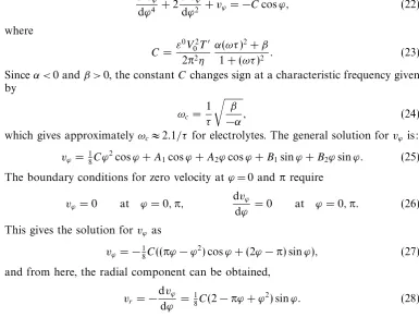
In this self-similar solution, the velocity components do not depend on the distance to the originr. Figure 2(a) shows a contour plot of a streamfunction, defined by the relations

vr =−

1 r

∂ ψ

∂ϕ, vϕ = ∂ ψ

∂r . (29)

The arrows indicate the direction of the fluid flow when the temperature decreases with height and the frequency is less than ωc as defined by (24). Forω > ωc, the flow

changes direction. The pattern of streamlines is very close to that given in Green et al. (2001) for a similar numerical problem in the neighbourhood of r = 0 where the self-similar solution is expected to be valid.

–2 –1 0 1 2 0

1 2 3 4

x z

(a) (b)

–0.04 –0.02 0.02 0.04 0.01

0.02 0.03 0.04

0.05 _v/C

Figure 2.(a) Streamlines for a vertically imposed temperature gradient. The arrows indicate

the direction of the fluid flow when the temperature decreases with height and the frequency is less thanωc. (b) Liquid speed as a function of angleϕfor a vertically imposed temperature gradient (polar curve).

(2001) for a system of two coplanar electrodes heated by light. In this work, the numerically calculated thermal field shows an almost vertical gradient of temperature over the electrodes. Using the values specified in Greenet al.(2001),T= 0.021 Kµm−1_, V0= 10 V and ωωc, the maximum radial velocity from the analytical solution is

87.0µms−1_{, compared to 80µms}−1 _{obtained from numerical work using finite-element} modelling.

3.2. Horizontal gradient

Assume now an imposed horizontal gradient of temperature in thex direction,∇T = Tux. In polar coordinates, this is

T(r, ϕ) =T0+Trcosϕ, (30)

where the temperature at the planeϕ=π/2 (orx= 0) is T0.

Assuming again that the permittivity and conductivity increments with temperature are small enough, we can write the electrical body force as:

f =−ε 0

2

V0 πr

2 T

α−β 1 + (ωτ)2 −

α 2

sinϕuϕ+ α

2cosϕur

, (31)

whereαand β have the same meaning as before.

Since the body force tends again as r−2_{, we can propose self-similar solutions as} previously. The resulting equation for the azimuthal velocity is now

d4_v ϕ

dϕ4 + 2 d2_v

ϕ

dϕ2 +vϕ =Csinϕ, (32)

whereC is the same constant as given in (23).

The solution forϕ that satisfies the boundary conditions for zero velocity at ϕ= 0 andπis

vϕ = 1₈C(πϕ−ϕ2) sinϕ. (33)

The expression for the radial component is

–2 –1 0 1 0

1 2 3 4

x z

(a) (b)

–0.2 –0.1 0.1 0.2 0.1

0.2 0.3

v/C

2

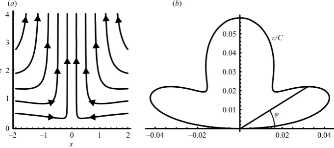
Figure 3. (a) Streamlines for a horizontally imposed temperature gradient. The arrows indicate

the direction of the fluid flow when the temperature decreases withx(to the right in the figure) andω < ωc. (b) Liquid speed as a function of angleϕ for a horizontally imposed temperature gradient (polar curve).

Figure 3(a) shows a contour plot of the corresponding streamfunction. The arrows indicate the direction of the fluid flow when the temperature decreases with x (to the right in the figure) and ω < ωc. As before, for ω > ωc the flow changes direction.

Figure 3(b) shows the modulus of the velocity for the same system. This solution is relevant to experiments where a difference in temperature is established between coplanar electrodes, producing a horizontal gradient (Green et al. 2000, 2001). Since unidirectional motion is obtained, this configuration could be used as the basis for a micro-pump employing only a single a.c. signal. For example, an array of interdigitated electrodes with a modulated temperature field could be used. An advantage of this type of pump is that for saline solutions, the maximum flow velocity is almost independent of the conductivity of the solution. In effect, the peak velocity is obtained at frequencies ωωcand it is proportional toβ= (dσ/dT)/σ. In order to avoid complications with

double-layer effects, the frequency of the applied signal should be increased linearly with conductivity, keeping ωωc.

The maximum absolute value ofvϕ is obtained atϕ=π/2, where vϕ= 0.308425C.

The maximum absolute value of vr is at ϕ1= 0.729827 and ϕ2=π −ϕ1 where vr(ϕ1) =−0.304156C andvr(ϕ2) = 0.304156C.

4. Three-dimensional fluid rotation

Extending the analysis to three dimensions, we consider a system of four electrodes placed at each quadrant, with small gaps in between, and with a rotating-phase voltage applied (see figure 1b).

In this system, the electric field has a net rotation around the z-axis. The induced volume charge density follows the field with a certain delay. The resulting volume force produces a torque on the liquid and the appearance of rotation of the fluid around a central axis.

4.1. Basic electric field

In the lowest order, the electric potential satisfies Laplace’s equation with the boundary condition at the planez= 0

φ =Vs(x, y, t)

⎧ ⎪ ⎨ ⎪ ⎩

V0cos(ωt), x >0, y >0, −V0sin(ωt), x <0, y >0, −V0cos(ωt), x <0, y <0, V0sin(ωt), x >0, y <0,

(35)

and with the potential vanishing far from the electrodes

φ→0 (z→ ∞). (36)

This problem can be posed in terms of the complex potential amplitude, that also satisfies Laplace’s equation, with the boundary condition

φ(z= 0) =Vs =

⎧ ⎪ ⎨ ⎪ ⎩

V0, x >0, y >0, V0i, x <0, y >0, −V0, x <0, y <0, −V0i, x >0, y <0.

(37)

The surface voltage can be written in a simpler form as follows

Vs=

V0(1−i)

2 sgn (x) +

V0(1 + i)

2 sgn (y), (38)

which corresponds to the symbolic equation:

i 1

−1 −i

= ₋ 1−i 2

1−i

2 +

1 + i 2

−1 + i

2

.

Each term of (38) is exactly the surface potential for the two-dimensional case that was described in the previous section. In this way, we can write the electric potential in the bulk as a sum of two two-dimensional solutions. These solutions are shifted 90◦ in space and in time, producing the rotating potential. Writing the angles in terms of Cartesian coordinates we have

φ = V0(1−i) π arctan

x z

+V0(1 + i) π arctan y z . (39)

The total complex amplitude for the electric field can also be expressed as a super-position of two fields

E0=

V0(1−i) π

−zux+xuz x2_+z2

+V0(1 + i) π

−zuy+yuz y2_+z2

The direction of the electric field (in the time domain) rotates, although not uniformly. This field can be written equivalently as

E0= 1−i

√

2 Ea+ 1 + i

√

2 Eb, (41)

with Ea and Eb purely real, multiplied by complex coefficient of unit modulus. The

first component is

Ea = V0

√

2 π

−zux+xuz x2_+z2

, (42)

which is identical to the two-dimensional field given in (18) except for the factor√2.

4.2. The case of a vertical gradient

We now consider the combined action of the previous electric field with an imposed uniform vertical temperature gradient, ∇T =Tuz.

The volume force

f = 1 2Re

ε0_(α−β)

1 + iωτ (∇T ·E0)E

∗

0

−ε0α

4 (E0·E

∗

0)∇T , (43)

and is composed of a Coulomb part and a dielectric one. Both can be decomposed into four terms, according to the components, Ea and Eb, of the electric field involved

f = f_aa+ f_ab+ f_ba+ f_bb. (44)

The first and last terms produce purely two-dimensional motions, as described in a previous section: f_aa generates a two-dimensional motion with components in the (x, z)-plane, and f_bb in the (y, z)-plane. The velocity expressions for these lateral motions are the same as in (27) and (28) multiplied by a factor 2. In what follows, we are mostly concerned with the cross-terms, fab and fba, which produce net rotation.

The cross-terms for the dielectric force cancel each other

f_d =−ε 0_α

4 ∇T(iEb·E

∗

a−iEa·E∗b) = 0. (45)

The only new terms appear in the Coulomb force:

fab+ fba=

ε0_{(α−β)ωτ}

(1 +ω2_τ2₎ ((∇T ·Ea)Eb−(∇T ·Eb)Ea). (46)

Even before calculating the spatial dependence of the coupled volume force density, we can establish the dependence on the frequency as

f_ab+ f_ba= ωτ

1 +ω2_τ2C. (47)

This term vanishes for low and high frequencies, with a maximum at the charge relaxation frequencyω=σ0_/ε0_{. Contrary to the previous two-dimensional fluid flows,} this three-dimensional case does not change direction with frequency.

The spatial dependence of the coupled force density is

f_c= Az(−yux+xuy)

(x2_+z2_)(y2_+z2₎, A=−

V₀2T(α−β)ε0ωτ

π2_{(1 +ω}2_τ2₎ , (48)

f_c= Acosθsinθ r2_(cos2_{θ+ sin}2

θcos2_ϕ)(cos2_{θ+ sin}2

θsin2ϕ)uϕ. (49)

This force is directed along the azimuthal direction, causing rotation.

The dependence on the angular coordinate ϕ is periodic with a period of length π/2, repeating each quadrant, and therefore it can be written as a Fourier series,

fc=

∞

n=−∞

cnei4nϕ. (50)

A somewhat lengthy calculation leads to the coefficients

cn=

2Asinθ r2_{(1 + cos}2_θ)

tan

θ 2

_|n_|

. (51)

Only the zero-order term produces net rotation. The component of this mode is obtained by averaging inϕ over a period

1 2π

2π

0

fcdϕ=c0 =

2Asinθ

r2_{(1 + cos}2_θ). (52)

Multiplying the Navier–Stokes equations byuϕand averaging inϕ, we obtain an

equ-ation for the mean azimuthal velocity

1 r

∂2

∂r2(rvϕ ) + 1 r2 ∂ ∂θ 1 sinθ ∂

∂θ(sinθvϕ )

=− 2Asinθ

ηr2_{(1 + cos}2_θ). (53)

As in the previous sections, the r−2-dependence of the force dictates the functional form for the self-similar velocity solution. We assume a functional form independent of r asvϕ =U(θ)A/η, which reduces the problem to an ordinary differential equation,

d dθ 1 sinθ d

dθ (sinθ U)

=− 2 sinθ

1 + cos2_θ. (54)

The solution for this equation that satisfies the b.c. of zero velocity at θ= 0 and at θ=π/2 is

U = cotθ

π

2−2 arctan(cosθ)−ln(2)

+ln(1 + cos 2_θ)

sinθ . (55)

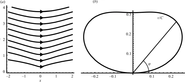
This function is always positive, and goes from zero at the axis to zero at the electrodes, reaching maximum speed atθ= 0.961 with a value Umax= 0.232 (see figure 4).

5. Comparison with experiments

0.5 1.0 1.5 0.1

0.2

θ U

Figure 4. Plot of the velocity functionU, (equation (55)), with polar angle θ.

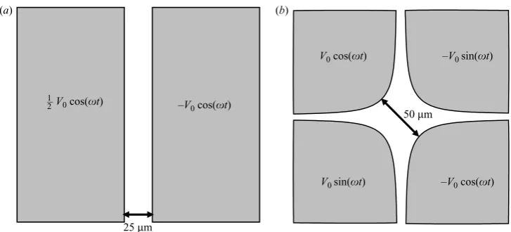
50 µm

25 µm

V0 cos(ωt)

1

– V₀cos(ωt)

2 –V0 cos(ωt)

–V0 sin(ωt)

–V0cos(ωt)

V0 sin(ωt)

(a) (b)

Figure 5.Diagram showing the two designs of electrode use in the experiments, with the

voltage sequences used to drive the fluid.

50µm

Electrodes

Lid

Figure 6.Horizontal view of two counter-rotating rolls on top of two coplanar electrodes at

V0= 7 V andf= 1 MHz. Image of particle tracks obtained by superimposing successive video frames.

and no observable motion was detected without electric fields. However, with the application of electric fields under illumination, fluid flow was observed in chambers with heights smaller than 200µm. The buoyancy force becomes less important as the typical system length decreases. As discussed by Castellanoset al.(2003), a transition between buoyancy and electrothermal fluid flows is expected to occur for typical system lengths around 300µm.

The magnitude of the incident light could be altered by inserting a filter into the light path. The light intensity was measured at different positions in the area of view using a photodiode. With a filter inserted into the light path, the light intensity decreased by a factor 3.62±0.15. If the flow is electrothermal in origin, i.e. if the conductivity and permittivity gradients occur because of light-induced heating of the liquid, then the velocity of the liquid is expected to change by the ratio of light intensity with and without the filter.

5.1. Experiments with a pair of symmetric electrodes

Observations of fluid flows under conditions similar to the two-dimensional problems previously analysed have been reported in Greenet al.(2000). Fluid flow was observed when the electrodes were subjected to voltages around 10 V and frequencies around 1 MHz under strong illumination. The observed fluid flow pattern agrees well with the prediction from the electrothermal theory if there is a vertical gradient of temperature, generated by the light (Green et al. 2001). The experimental fluid flow changed direction at a certain frequency and the fluid velocity amplitude varied with frequency as predicted. The two-dimensional analytical solutions of the present work compare well with the numerical and experimental results.

y = 3.38x1.94

y = 1.25x1.96

100

101 102 103

100 ₁₀1

(a) (b)

Applied voltage (V)

Velocity (

µ

m s

–1)

Figure 7. Best-fit power law of velocity against applied voltage at_f= 1 MHz: (a) two coplanar

electrodes subjected to a single phase signal, and (b) four coplanar electrodes subjected to a four-phase signal.

with a filter. This factor corresponds to the ratio of light intensities with and without the filter, and indicates that the flow is electrothermal.

The velocity as a function of voltage amplitude V0 at the same position and frequency is shown in figure 7. The best-fit power curve is given byu= 1.25V1.96

0 µm s−1 (with V0 in volts), close to the expected power law u∝V02. At this height of 77µm, dielectrophoresis on the tracking particles should be negligible (Ramos et al. 1998). A maximum estimated dielectrophoretic velocity is around 0.01V₀2µm s−1_{, much} smaller than the measured velocities.

In previous experiments (Greenet al.2000), with a voltage ofV0= 10 V the velocity was found to be 80µm s−1_{. In the present work, we measured a value of 110µm s}−1 for the same voltage. This discrepancy could be explained by a change in the vertical temperature gradient, by a factor 1.37 times greater than in the previous experiments.

5.2. Experiments on electrothermal rotation

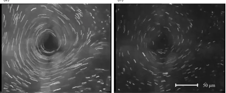
Figure 8 shows particle tracks at a plane 40µm up from the electrodes for two cases: (a) with maximum incident light, and (b) with the light intensity reduced by a factor 3.6 with a filter. The electrodes were driven with a four-phase sine wave with a voltage amplitude of V0= 6 V and a frequency of f = 3 MHz. The particle trajectories demonstrate that the liquid rotates when subjected to a rotating electric field under strong illumination. When the direction of the rotating field was changed, the liquid changed direction accordingly. Because there is more light in case (a), the particle track lengths are greater than in case (b) for the same time interval. The ratio between measured velocities at selected points in case (a) and in case (b) is 3.4±0.2, in agreement with the ratio of light intensities.

Figure 7 shows the velocity as a function of voltage, measured at a radius of 100µm from the centre of rotation, a height of 30µm above the electrodes, and a frequency of 1 MHz. The best-fit power curve is given by u= 3.38V1.94

50 µm

(a) (b)

Figure 8.Top view of a rotating aqueous solution placed on top of four coplanar electrodes.

Image of particle tracks obtained by superimposing successive video frames in a time interval of 0.4 s: (a) maximum light intensity, and (b) light intensity reduced by filter.

96±9µm s−1 _{at V}

0= 5.4 V and 1 MHz. In order to obtain this velocity using the analytical expression, the temperature gradient should be ofT= 0.025 Kµm−1_{. This} gradient of temperature is 1.2 times greater than the gradient estimated in previous experiments (Greenet al. 2000, 2001).

As predicted by the three-dimensional analytical solution, the rotating fluid flow was significant over a certain frequency range and did not change direction with frequency. Figure 9 shows particle tracks from a top view at V0= 5.8 V and four different frequencies: 0.2, 0.5, 2 and 5 MHz. The fluid flow behaves differently at frequencies above and below 1 MHz. Above 1 MHz, the flow patterns are more circular, while below 1 MHz they look like spirals. According to the theory, the flow is the sum of two superimposed characteristic fluid flows: (a) a rotating flow with maximum rotation atf= 0.568 MHz as given byω=σ/ε; and (b) two superimposed two-dimensional flows with velocity components in the (x, z)- and (y, z)-planes, and with a characteristic frequency of 1.27 MHz as given by ωc= (σ/ε)

√

−β/α. At this frequency, the two-dimensional flows disappear because Coulomb and dielectric forces cancel each other. The ratio between two-dimensional and rotational velocities is proportional to

v2D vrot ∝

|β− |α|(ωτ)2_|

(β+|α|)ωτ . (56)

This ratio is zero for the transition frequency ωc. For very high and very low

frequencies, the two-dimensional motions dominate. There is an interval of frequencies aroundωcwhere the rotational motion is dominant. Forωωc, the two-dimensional

motion is proportional to β whereas for ωωc, the two-dimensional motion is

proportional to|α| ∼ |β|/5. Therefore, the frequency range where rotation is dominant is greater for ω > ωc than for ω < ωc. This can explain why the spiral-like paths

observed at f <1 MHz change to more circular paths at f >1 MHz, since the two-dimensional motions are relatively less important at these frequencies.

(a) (b)

(c) (d)

Figure 9. Top view of a rotating aqueous solution on top of four coplanar electrodes. The

applied four-phase signals have an amplitude of 5.8 V and different frequencies: (a) 0.2 MHz, (b) 0.5 MHz, (c) 2 MHz and (d) 5 MHz.

0 0.1 0.2 0.3 0.4 0.5 0.6

10–1 ₁₀0 ₁₀1

Frequency (MHz)

Angular velocity (rad s

–1)

Figure 10. Angular velocity as a function of frequency.

this case (see figure 9). Theoretically, the maximum angular velocity is obtained at f=σ0/2πε0= 0.568 MHz, in accordance with the experiments within experimental errors. The theoretical expression for the angular velocity at a given height h from the electrodes is given by

Ω(θ) = A

hηU(θ) cotθ. (57)

The illumination intensity was different from the previous experiments and the measured angular velocities would be obtained if the temperature gradient is around four times smaller than for the data shown in figure 7.

6. Conclusions

Self-similar solutions for the fluid flow induced by the combination of electric fields and externally imposed gradients of temperature in microelectrode structures have been presented. Two kinds of problem were considered: (a) the two-dimensional motion of an aqueous solution placed on top of two coplanar parallel electrodes subjected to an a.c. potential difference when there is either a vertical or a horizontal gradient of temperature; and (b) the three-dimensional motion of an aqueous solution lying on four coplanar hyperbolic electrodes subjected to a four-phase a.c. signal, generating a rotating electric field.

Experiments were performed using aqueous solutions of KCl placed on top of two or four coplanar microelectrodes and the results compared with the analytical solutions. The temperature field was imposed using the light from the microscope. Indications of this were the observation of natural convection for devices with heights around 1 mm and that the observed electrothermal fluid velocities were proportional to the light intensity. The device with two coplanar parallel electrodes produced two-dimensional rolls of fluid flow. The device with four hyperbolic electrodes demonstrated that the liquid rotates when subjected to a rotating electric field under strong illumination. The experiments showed a good agreement with the expected trends from the theoretical solutions.

The combination of electric fields and heating with light at localized points could be of interest in the design of micro-pumps and for local mixing in the lab-on-a-chip technology. An advantage of this way of generating flow in saline solutions is that the maximum flow velocity is almost independent of the conductivity of the solution. In order to obtain the best efficiency, the frequency of the applied signal should be increased linearly with conductivity.

This work has been supported by the Spanish MCyT, under contract BFM2003-01739.

R E F E R E N C E S

Ajdari, A.2000 Pumping liquids using asymmetric electrode arrays.Phys. Rev.E61, R45–R48.

Arnold, W. M.2001 Positioning and levitation media for the separation of biological cells.IEEE

Trans. Ind. Applics37, 1468–1475.

Bazant, M. Z. & Squires, T. M. 2004 Induced-charge electrokinetic phenomena: theory and

microfluidic applications.Phys. Rev. Lett.92, 066101.

Bazant, M. Z., Thornton, K. & Ajdari, A. 2004 Diffuse-charge dynamics in electrochemical

systems.Phys. Rev.E70, 021506.

Castellanos, A. 2003 Entropy production and the temperature equation in

Castellanos, A., Ramos, A., Gonz ´alez, A., Green, N. G. & Morgan, H. 2003 Electro-hydrodynamics and dielectrophoresis in microsystems: scaling laws. J. Phys.D:Appl. Phys.

36, 2584–2597.

Chen, H.-H., Lin, H., Lele, S. K. & Santiago, J. G. 2005 Convective and absolute electrokinetic

instability with conductivity gradients.J. Fluid Mech.524, 263–303.

Gimsa, J., Eppmann, P. & Pr¨uger, B.1997 Introducing phase analysis light scattering for dielectric

characterization: measurement of travelling-wave pumping.Biophys. J.73, 3309–3316.

Green, N. G., Ramos, A., Gonz ´alez, A., Castellanos, A. & Morgan, H. 2000 Electric field

induced fluid flow on microelectrodes: the effect of illumination.J. Phys.D:Appl. Phys.33, L13–L17.

Green, N. G., Ramos, A., Gonz ´alez, A., Castellanos, A. & Morgan, H._{2001 Electrothermally}

induced fluid flow on microelectrodes.J. Electrost.53, 71–87.

Haus, H. A. & Melcher, J. R.1989Electromagnetic Fields and Energy. Prentice-Hall.

Levich, V. G.1962Physicochemical Hydrodynamics.Prentice-Hall.

Lide, D. R.(ed.) 1994CRC Handbook of Chemistry and Physics, 74th edn. CRC Press, London.

Melcher, J. R.Continuum Electromechanics. 1981 The MIT Press, Cambridge, MA.

Melcher, J. R. & Firebaugh, M. S.1967 Traveling-wave bulk electroconvection induced across a

temperature gradient.Phys. Fluids 10, 1178–1185.

Melcher, J. R. & Taylor, G. I. 1969 Electrohydrodynamics: a review of the role of interfacial

shear stresses.Annu. Rev. Fluid Mech.1, 111–146.

M¨uller, T., Arnold, W. M., Schnelle, T., Hagedorn, R., Fuhr, G. & Zimmermann, U.1993

A traveling-wave micropump for aqueous solutions: comparison of 1 g andµg results. Electrophoresis14, 764–772.

M¨uller, T., Gerardino, A., Schnelle, Th., Shirley, S. G., Bordoni, F., De Gasperis, G., Leoni,

R. & Fuhr, G.1996 Trapping of micrometre and sub-micrometre particles by high-frequency

electrical fields and hydrodynamic forces.J. Phys.D:Appl. Phys.29, 340–349.

Putnam, S. A. & Cahill, D. G.2005 Transport of nanoscale latex spheres in a temperature gradient.

Langmuir 21, 5317–5323.

Ramos, A., Morgan, H., Green, N. G. & Castellanos, A.1998 AC electrokinetics: a review of

forces in microelectrode structures.J. Phys.D:Appl. Phys.31, 2338–2353.

Ramos, A., Morgan, H., Green, N. G. & Castellanos, A.1999 AC electric-field-induced fluid flow

in microelectrodes.J. Colloid Interface Sci.217, 420–422.

Saville, D. A.1997 Electrohydrodynamics: the Taylor–Melcher leaky dielectric model.Annu. Rev.

Fluid Mech.29, 27–64.

Schnelle, T., M¨uller, T., Reichle, C. & Fuhr, G. 2000 Combined dielectrophoretic field cages

and laser tweezers for electrorotation.Appl. Phys.B70, 267–274.

Tritton, D. J.1977Physical Fluid Dynamics. Van Nostrand Reinhold.

Wang, D., Sigurdson, M. & Meinhart, C. D. 2005 Experimental analysis of particle and fluid