Sparse Kernel Density Construction Using
Orthogonal Forward Regression With
Leave-One-Out Test Score and
Local Regularization
Sheng Chen
, Senior Member, IEEE
, Xia Hong
, Senior Member, IEEE
, and Chris J. Harris
Abstract—This paper presents an efficient construction algo-rithm for obtaining sparse kernel density estimates based on a regression approach that directly optimizes model generalization capability. Computational efficiency of the density construction is ensured using an orthogonal forward regression, and the algorithm incrementally minimizes the leave-one-out test score. A local regularization method is incorporated naturally into the density construction process to further enforce sparsity. An additional advantage of the proposed algorithm is that it is fully automatic and the user is not required to specify any criterion to terminate the density construction procedure. This is in contrast to an existing state-of-art kernel density estimation method using the support vector machine (SVM), where the user is required to specify some critical algorithm parameter. Several examples are included to demonstrate the ability of the proposed algorithm to effectively construct a very sparse kernel density estimate with comparable accuracy to that of the full sample optimized Parzen window density estimate. Our experimental results also demonstrate that the proposed algorithm compares favorably with the SVM method, in terms of both test accuracy and sparsity, for constructing kernel density estimates.
Index Terms—Cross validation, leave-one-out test score, orthog-onal least squares, Parzen window estimate, probability density function, regularization, sparse kernel modeling.
I. INTRODUCTION
E
STIMATION of probability density functions is a recur-rent theme in machine learning and many fields of engi-neering, see for example [1]–[4]. A well-known nonparametric density estimation technique is the classical Parzen window es-timate [5], which is remarkably simple and accurate. The partic-ular problem associated with the Parzen window estimate how-ever is the computational cost for testing which scales directly with the sample size, as the Parzen window estimate employs the full data sample set in defining a density estimate for sub-sequent observations. In today’s data-rich environment, this can be a serious problem in practical applications. Recently, the sup-port vector machine (SVM) has been proposed as a promisingManuscript received December 23, 2003; revised March 18, 2004. This paper was recommended by Associate Editor D. D. Nauck.
S. Chen and C. J. Harris are with School of Electronics and Computer Science, University of Southampton, Southampton SO17 1BJ, U.K. (e-mail: [email protected]).
X. Hong is with Department of Cybernetics, University of Reading, Reading RG6 6AY, U.K.
Digital Object Identifier 10.1109/TSMCB.2004.828199
tool for sparse kernel density estimation [6], [7]. The motivation of the SVM density estimation comes from the claim that the SVM can effectively perform function approximations in high dimensional spaces from finite data with sparse representations. Although this effectiveness has been demonstrated in regression and classification problems, it is known that there are alternative methods for regression and classification [8], [9], which can pro-vide sparser representations than the SVM method. Currently, the machine learning community is actively engaged in the in-vestigation of the SVM density estimation method.
A recent Ph.D. dissertation [10] has proposed an interesting greedy technique for kernel density estimation. This technique constructs sparse kernel density estimates using an orthogonal forward regression (OFR) that incrementally minimizes the training mean square error (MSE) [11]. This sparse density construction algorithm is computationally simple and efficient, and the results given in [10] have demonstrated the potential of this method. One critical aspect of this method, which is less satisfactory, is in when to terminate the density construction procedure. The minimum descriptive length [12] and Akaike’s information criterion [13] were first suggested to help terminate the density construction process, but the empirical results showed that models obtained were still often oversized. At the end, a maximum model size was imposed in order to avoid an over-fit model. Motivated by the promising result in [10] and our previous work on sparse data modeling [14]–[16], we propose an efficient construction algorithm for sparse kernel density estimation using the OFR based on the leave-one-out (LOO) test score and local regularization. Specifically, we extend the regression model construction algorithm [16] to the construction of sparse kernel density estimates. We will refer to our proposed algorithm as the sparse density construction (SDC) algorithm.
Our motivation is twofold. Firstly, we aim to derive sparse kernel density estimates based on optimizing model general-ization capability or test performance. We also want the kernel density construction process to be automatic without the need for the user to specify some additional termination criterion. The usual training MSE cannot achieve these objectives, but the delete-one cross validation with its associated LOO test score [17]–[20] provides the capability to achieve this aim, without resorting to use a separate validation data set. Secondly, the level of sparsity and computational efficiency are also critical
to the kernel density construction process. The computational efficiency of using the delete-one cross validation is ensured by using the orthogonal least squares algorithm [21], [22], as is first shown in [20], and multiple-regularizers or local regulariza-tion is known to be capable of providing very sparse soluregulariza-tions [8], [14]–[16]. Our previous work on sparse regression mod-eling [16] has shown that the OFR based on the LOO test score and local regularization offers considerable advantages in real-izing these two critical objectives of sparse modeling over sev-eral other state-of-art methods. The current investigation shows that the proposed SDC method inherits these crucial advan-tages. Compared with the SVM method, our SDC algorithm is simpler to implement and has no critical algorithm param-eter that needs to be specified by the user. Several examples are used to illustrate the ability of this new SDC algorithm to con-struct efficiently a sparse density estimate with comparable ac-curacy to that of the Parzen window estimate. Some examples that have been used in the existing literature to investigate the SVM method are specifically chosen in order to compare the performance of our SDC algorithm with the SVM density esti-mation method. Our experimental results demonstrate that the SDC algorithm offers a viable alternative to the SVM method for constructing sparse and accurate kernel density estimates.
II. KERNELDENSITYESTIMATION ASREGRESSION
Consider the finite sample set drawn from a density , where the data samples
are assumed to be inde-pendently identically distributed. The task is to estimate the unknown density using the kernel density estimate of the form
(1)
with the constraints
(2) and
(3)
In this study, the kernel function is assumed to be the Gaussian function of the form
(4) where is a common kernel width. The well-known Parzen window estimate [5] is obtained by setting for all . Our aim is to seek a spare representation for , i.e., with most of being zero and yet maintaining a comparable test per-formance or generalization capability to that of the full sample Parzen window estimate having an optimized value for .
A density is defined as the solution of
(5)
subject to the constraints
(6) and
(7) where is the unknown cumulative distribution function corresponding to the density . Given the data set , the empirical distribution function defined by
(8)
with
(9) is known to be a good approximation to the true distribution function [6], [7]. Thus, the kernel density estimation problem can be posed as the following regression modeling problem [6], [7], [10]:
(10) subject to the constraints (2) and (3), where the “regressor”
is given by
(11)
with
(12) and denotes the modeling error at .
Define , and
with . Then the regression model (10) for the data point can be expressed as
(13) where . Furthermore, the regression model (10) over the training data set can be written together in the matrix form
(14) with the following additional notations ,
with , and
. For convenience, we will denote the regression
matrix with .
should not be confused with (the former is the th column of , and the latter the th row of ). Let an orthogonal decom-position of the regression matrix be
where
. .. ... ..
. . .. ...
(16)
and
(17) with columns satisfying , if . The regression model (14) can alternatively be expressed as
(18) where the weight vector associated with the orthogonal space satisfies the triangular system . The space spanned by the original model bases , is identical to the space spanned by the orthogonal model bases , and the model is equivalently expressed by (19) where is the th row of .
In general, the “regression” matrix in (14) may be ill-con-ditioned or even noninvertible, particularly for a large data set. This can cause numerical problems for some density construc-tion algorithms, but not the proposed SDC algorithm. This is be-cause the OFR automatically avoids any ill-conditioning prob-lems and selects a subset matrix of that is well-conditioned.
III. SPARSEDENSITYCONSTRUCTION
In the OFR algorithm based on the LOO test score and local regularization [16], the weight parameter vector is the regu-larized least squares solution obtained by minimizing the fol-lowing regularized error criterion:
(20)
where is the regularization parameter vector, which is optimized based on the evidence procedure [23] with the iterative updating formulas [15], [16]
(21) where
(22) Usually a few iterations (typically less than ten) are sufficient to find a local optimal . The criterion (20) has its root in the Bayesian learning framework. For the completeness, this Bayesian interpretation of together with the deriva-tion of the updating formulas (21) and (22) are summarized in Appendix A.
An OFR procedure is used to construct a sparse density esti-mate by incrementally minimizing the LOO test score. Assume that an -term model is selected from the full model (18). Then
the LOO test error [17]–[20], denoted as , for the se-lected -term model can be shown to be [16], [20]
(23) where is the -term modeling error and is the as-sociated LOO error weighting given by
(24) The mean square LOO error for the model with a size is de-fined by
(25) This LOO test score can be computed efficiently due to the fact that the -term model error and the associated LOO error weighting can be calculated recursively according to
(26) and
(27) respectively. For the benefits of those readers who are unfamiliar with the LOO statistics, the idea of delete-1 cross validation and the computation of the LOO test error are explained in Ap-pendix B.
The subset model selection procedure can be carried as fol-lows: at the th stage of the selection procedure, a model term is selected among the remaining to candidates if the re-sulting -term model produces the smallest LOO test score . It has been shown in [20] that the LOO statistic is convex with respect to the model size . That is, there exists an “op-timal” model size such that for decreases as increases while for increases as increases. This property is extremely useful, as it enables the selection pro-cedure to be automatically terminated with an -term model when , without the need for the user to specify a separate termination criterion. The iterative SDC procedure based on this OFR with LOO test score and local regularization can now be summarized as follows.
Initialization: Set , to the same small positive value (e.g., 0.001). Set iteration index .
Step 1) Given the current and with the following initial conditions:
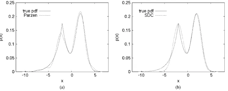
Fig. 1. (a) True density (solid) and a Parzen window estimate (dashed) and (b) true density (solid) and a sparse density construction estimate (dashed), for the 1-D example.
Step 2) Update using (21) and (22) with . If remains sufficiently unchanged in two successive iterations or a preset maximum iteration number (e.g., 10) is reached, stop; otherwise set and go toStep 1.
The computational complexity of the above algorithm is dom-inated by the 1st iteration. After the first iteration, the model set contains only terms, and the complexity of the subse-quent iteration decreases dramatically. As a probability density, the constraint (2) must be met. In [10], the nonnegative condi-tion (2) is guaranteed by using backward eliminacondi-tion. Let be the subset matrix of , corresponding to the -term model, and and the associated orthogonal and original weight vectors, respectively, linked by . If adding the th term causes some of the elements in to become negative, the associated previously selected model terms are removed. This strategy requires to carry out re-orthogonalization and in par-ticular re-calculation of the LOO test score, which are compu-tationally expensive. We adopt a much simple method to guar-antee the nonnegative condition (2). In the th stage, a candidate that causes to have negative elements, if included, will not be considered at all. The unit length condition (3) can easily be met by normalizing the final -term model weights with
(29)
IV. NUMERICALEXAMPLES
Four examples were used in simulation to test the proposed SDC algorithm and to compare its performance with the Parzen window estimate. Comparison with SVM kernel density esti-mation was also given by quoting the results of [7]. In order to remove the influence of different values to the quality of the resulting density estimate, the optimal value for , found empir-ically by cross validation, was used. That is, the value of used was determined by testing performance. For the first three ex-amples, in each case, a data set of randomly drawn samples was used to construct kernel density estimates, and a separate
TABLE I
PERFORMANCE OF THEPARZENWINDOW(PW) ESTIMATE AND THE
PROPOSEDSPARSEDENSITYCONSTRUCTION(SDC) ALGORITHM FOR THE
1-D EXAMPLE. STD: STANDARDDEVIATION
test data set of samples was used to calculate the test error for the resulting estimate according to
(30)
The experiment was repeated by 100 different random runs for each example. The fourth example was a two-class two-dimen-sional (2-D) classification problem taken from [24].
Example 1: This was a one-dimensional (1-D) example, and the density to be estimated was given by
(31) The number of data points for density estimation was . The optimal kernel widths were found to be and empirically with cross validation for the Parzen window estimate and the SDC estimate, respectively. Table I compares the performance of the two kernel density construction methods, in terms of the test error and the number of kernels required. Fig. 1(a) depicts the Parzen window estimated obtained in a run while Fig. 1(b) shows the density obtained by the SDC algo-rithm in a run, in comparison with the true distribution. For this 1-D example, it can be seen that the accuracy of the proposed SDC algorithm was comparable to that of the Parzen window estimate, and the algorithm realized very sparse estimates with an average kernel number less than 5% of the data samples.
This example was considered in [7], where a SVM Gaussian kernel density estimate of five terms was identified from a single set of 100 training data with an test error of
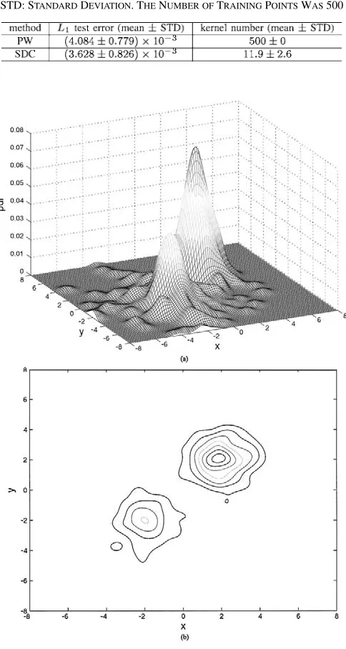
Fig. 2. (a) True density and (b) contour plot for the 2-D example.
obtained by the SDC method compares favorably with that of SVM method.
Example 2: The density to be estimated for this 2-D example was defined by
(32) Fig. 2 shows this density distribution and its contour plot. The estimation data set contained samples, and the em-pirically found optimal kernel widths were for the Parzen window estimate and for the SDC estimate, respectively. Table II lists the test errors and the numbers of kernels required for the two density estimation methods. A typical Parzen window estimate and a typical SDC estimate are depicted in Figs. 3 and 4, respectively. Again, for this example, the two density construction methods had comparable accura-cies, but the SDC algorithm achieved very sparse estimates with an average number of required kernels less than 3% of the data samples.
TABLE II
PERFORMANCE OF THEPARZENWINDOW(PW) ESTIMATE AND THEPROPOSED
[image:5.612.308.550.92.546.2]SPARSEDENSITYCONSTRUCTION(SDC) ALGORITHM FOR THE2-D EXAMPLE. STD: STANDARDDEVIATION. THENUMBER OFTRAININGPOINTSWAS500
Fig. 3. (a) Parzen window estimate and (b) contour plot (b) for the 2-D example.
Fig. 4. (a) Sparse density construction estimate (a) and (b) contour plot for the 2-D example.
TABLE III
PERFORMANCE OF THEPARZENWINDOW(PW) ESTIMATE AND THEPROPOSED
SPARSEDENSITYCONSTRUCTION(SDC) ALGORITHM FOR THE2-D EXAMPLE. STD: STANDARDDEVIATION. THENUMBER OFTRAININGPOINTSWAS60
Example 3: In this six-dimensional (6-D) example, the un-derlying density to be estimated was given by
(33)
TABLE IV
PERFORMANCE OF THEPARZENWINDOW(PW) ESTIMATE AND THE
PROPOSEDSPARSEDENSITYCONSTRUCTION(SDC) ALGORITHM FOR THE
6–D EAMPLE: STD STANDARDDEVIATION
TABLE V
PERFORMANCE OF THEPARZENWINDOW(PW) ESTIMATE AND THE
PROPOSEDSPARSEDENSITYCONSTRUCTION(SDC) ALGORITHM FOR THETWO-CLASSCLASSIFICATIONPROBLEM
with
(34)
(35)
(36) The estimation data set contained samples. The op-timal kernel width was found to be for the Parzen window estimate and for the SDC estimate, respec-tively, via cross validation using the test data set. The results obtained by the two density construction algorithms are summa-rized in Table IV. It can be seen that the SDC algorithm achieved a similar accuracy to that of the Parzen window estimate with a much sparser representation. The average number of required kernels for the SDC method was less than 3% of the data sam-ples.
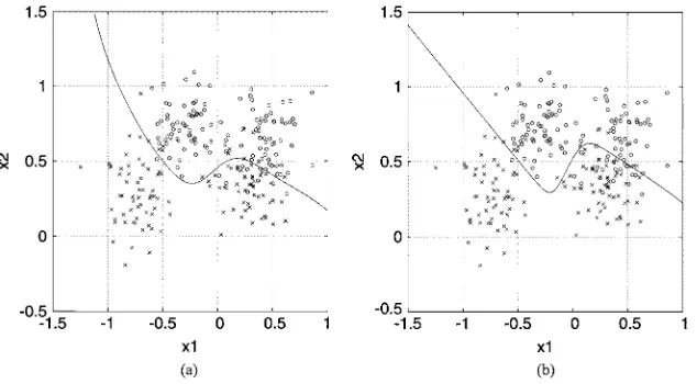
Example 4: The data was obtained from http://www.stats. ox.ac.uk/PRNN/. This was the synthetic data set taken from [24], which was a two-class classification problem in a 2-D fea-ture space. The training set contained 250 samples with 125 points for each class, and the test set had 1000 points with 500 samples for each class. Tipping [8] reported that the optimal Bayes error rate for this example is around 8%, who also con-structed a SVM Gaussian kernel classifier of 38 kernel functions with a test error rate of 10.6% and a relevance vector machine Gaussian kernel classifier of four kernel functions with a test error rate of 9.3%. We first estimated the two conditional den-sity functions and from the training data, and then applied the Bayes decision rule
if belongs to class 0
belongs to class 1 (37) to the test data set and calculated the corresponding error rate.
perfor-Fig. 5. (a) Decision boundary of the Parzen window estimate, and (b) decision boundary of the sparse density construction estimate, where circles represent the class-1 training data and crosses the class-0 training data.
mance. This clearly demonstrated the accuracy of the density estimates. This result compares favorably with the results of the state-of-art kernel classifiers reported in [8]. Fig. 5(a) and (b) de-pict the decision boundaries of the classifier (37) for the Parzen window and SDC methods, respectively.
V. CONCLUSION
An efficient construction algorithm has been presented for obtaining kernel density estimates based on an orthogonal forward regression procedure that incrementally minimizes the leave-one-out test score, coupled with local regularization to further enforce the sparseness of density estimate repre-sentations. The proposed method is simple to implement and computationally efficient, and except for the kernel width the algorithm contains no other free parameters that require tuning. The ability of the proposed algorithm to construct a very sparse kernel density estimate with a comparable accuracy to that of the full sample Parzen window estimate has been demonstrated using several examples. The results obtained have shown that the proposed method provides a viable alternative to the state-of-art support vector machine method for sparse kernel density estimation in practical applications.
APPENDIX A
According to the Bayesian learning theory (e.g., [8] and [23]), the optimal is obtained by maximizing the posterior proba-bility of , which is given by
(38)
where is the prior with de-noting the vector of hyperparameters and a noise parameter (the inverse of the variance of ), is the like-lihood, and is the evidence that does not depend on explicitly. Under the assumption that is white and has a Gaussian distribution, the likelihood is expressed as
(39)
If the Gaussian prior is chosen, namely
(40)
maximizing with respect to is equivalent to minimizing the following Bayesian cost function:
(41) where . It is easily seen that the cri-terion (20) is equivalent to the cricri-terion (41) with the relation-ship
(42) The hyperparameters specify the prior distributions of . Since initially one does not know the optimal value of
should be initialized to the same small value, and this corresponds to choose a same flat distribution for each prior of in (40). The beauty of Bayesian learning is “let data speak”—it learns not only the model parameters but also the related hyperparameters . This can be done for example by iteratively optimizing and using an evidence procedure [23], [8]. Following MacKay [23], it can be shown that the log model evidence for and is approximated as
log log log
log
(43) where is set to the maximum a posterior probability solution, and the “Hessian” matrix is diagonal and is given by
[image:7.612.141.458.60.235.2]Setting yields the recalculation formula for
(45)
Setting yields the recalculation formula for
(46)
Note and define
(47)
with
(48) Then the recalculation formula for is
(49)
APPENDIX B
Consider the model selection problem where a set of models have been identified using the training data set . Denote these models, identified using all the data points of , as and the corresponding modeling errors as
(50) with index . A commonly used cross validation for model selection is the delete-1 cross validation. The idea is as follows. For every model, each data point in the training set is sequentially set aside in turn, a model is estimated using the remaining data points, and the prediction error is de-rived using only the data point that was removed from training. Specifically, let be the resulting data set by removing the th data point from , and denote the th model esti-mated using as and the related predicted model residual at as
(51) The mean square LOO test error [17], [18] for the th model
is obtained by averaging all these prediction errors
(52)
The mean-square LOO test error is a measure of the model gen-eralization capability. To select the best model from the can-didate models , the same modeling procedure is applied to each of the predictors, and the model with the minimum LOO test error is selected.
For linear-in-the-weights models, the LOO test errors can be generated, without actually sequentially splitting the training data set and repeatedly estimating the associated models, by using the Sherman–Morrison–Woodbury theorem [17]. More-over, within the OFR model selection procedure, the LOO test errors for the -term model can be computed very efficiently. It can readily be shown in [16] and [20] that the computation of the LOO error for the -term model is based on the previously selected -term model and the currently se-lected th model term via the efficient recursion formulas (26) and (27).
APPENDIX C
The modified Gram-Schmidt orthogonalization procedure [21] calculates the matrix row by row and orthogonal-izes as follows: at the th stage make the columns
, orthogonal to the th column and repeat the operation for . Specifically, denoting
, then for
(53)
The last stage of the procedure is simply . The elements of are computed by transforming in a sim-ilar way
(54)
This orthogonalization scheme can be used to derive a simple and efficient algorithm for selecting subset models in a forward-regression manner [21]. First define
(55)
If some of the columns in have been interchanged, this will still be referred to as for nota-tional convenience. Let denote the subset matrix of , cor-responding to the -term model, and and the associated orthogonal and original weight vectors, respectively, satisfying . Let a very small positive number be given, which specifies the zero threshold and is used to automatically avoiding any ill-conditioning or singular problem. With the ini-tial conditions as specified in (28), the th stage of the selection procedure is given as follows.
Step 1) For :
Test 1—Conditioning number check. If
Test 2—Non-negativeness check. Compute
Set and solve for . If contains negative elements, the th candidate is not considered.
Compute, for
and
where and are the th elements of and , respectively. Let the index set be
and passes both Tests 1 and 2 Step 2) Find
Then the th column of is interchanged with the th column of , the th column of is in-terchanged with the th column of up to the th row, and the th element of is interchanged with the th element of . This effectively selects the th can-didate as the th regressor in the subset model. Step 3) The selection procedure is terminated with a
-term model, if . Otherwise, perform the orthogonalization as indicated in (53) to derive the th row of and to transform into ; calculate and update into in the way shown in (54); update the LOO error weightings
and go toStep 1.
REFERENCES
[1] C. M. Bishop,Neural Networks for Pattern Recognition, Oxford, U.K.: Oxford Univ. Press, 1995.
[2] B. W. Silverman,Density Estimation, London, U.K.: Chapman & Hall, 1996.
[3] H. Wang, “Robust control of the output probability density functions for multivariable stochastic systems with guaranteed stability,”IEEE Trans. Automat. Contr., vol. 44, pp. 2103–2107, Nov. 1999.
[4] S. Chen, A. K. Samingan, B. Mulgrew, and L. Hanzo, “Adaptive min-imum-BER linear multiuser detection for DS-CDMA signals in multi-path channels,”IEEE Trans. Signal Processing, vol. 49, pp. 1240–1247, June 2001.
[5] E. Parzen, “On estimation of a probability density function and mode,” Ann. Math. Statist., vol. 33, pp. 1066–1076, 1962.
[6] J. Weston, A. Gammerman, M. O. Stitson, V. Vapnik, V. Vovk, and C. Watkins, “Support vector density estimation,” inAdvances in Kernel Methods—Support Vector Learning, B. Schölkopf, C. Burges, and A. J. Smola, Eds. Cambridge, MA: MIT Press, 1999, pp. 293–306. [7] S. Mukherjee and V. Vapnik, “Support Vector Method for Multivariate
Density Estimation,” MIT AI Lab., Tech. Rep., A.I. Memo no. 1653, 1999.
[8] M. E. Tipping, “Sparse Bayesian learning and the relevance vector ma-chine,”J. Mach. Learn. Res., vol. 1, pp. 211–244, 2001.
[9] S. S. Chen, D. L. Donoho, and M. A. Saunders, “Atomic decomposition by basis pursuit,”SIAM Rev., vol. 43, no. 1, pp. 129–159, 2001. [10] A. Choudhury, Fast Machine Learning Algorithms for Large
Data. Southhampton, U.K.: Comput. Eng. Design Center, School Eng. Sciences, Univ. Southampton, 2002.
[11] P. B. Nair, A. Choudhury, and A. J. Keane, “Some greedy learning al-gorithms for sparse regression and classification with Mercer kernels,” J. Mach. Learn. Res., vol. 3, pp. 781–801, 2002.
[12] M. H. Hansen and B. Yu, “Model selection and the principle of minimum description length,”J. Amer. Stat. Assoc., vol. 96, no. 454, pp. 746–774, 2001.
[13] H. Akaike, “A new look at the statistical model identification,”IEEE Trans. Automat. Contr., vol. AC-19, pp. 716–723, 1974.
[14] S. Chen, “Locally regularised orthogonal least squares algorithm for the construction of sparse kernel regression models,” inProc. 6th Int. Conf. Signal Processing, Beijing, China, Aug. 26–30, 2002, pp. 1229–1232. [15] S. Chen, X. Hong, and C. J. Harris, “Sparse kernel regression modeling
using combined locally regularized orthogonal least squares and D-op-timality experimental design,”IEEE Trans. Automat. Contr., vol. 48, pp. 1029–1036, June 2003.
[16] S. Chen, X. Hong, C. J. Harris, and P. M. Sharkey, “Sparse modeling using orthogonal forward regression with PRESS statistic and regular-ization,”IEEE Trans. Syst., Man, Cybern. B, vol. 34, pp. 898–911, Apr. 2004.
[17] R. H. Myers,Classical and Modern Regression with Applications, 2nd ed. Boston, MA: PWS-KENT, 1990.
[18] L. K. Hansen and J. Larsen, “Linear unlearning for cross-validation,” Adv. Computat. Math., vol. 5, pp. 269–280, 1996.
[19] G. Monari and G. Dreyfus, “Local overfitting control via leverages,” Neural Comput., vol. 14, pp. 1481–1506, 2002.
[20] X. Hong, P. M. Sharkey, and K. Warwick, “Automatic nonlinear pre-dictive model construction algorithm using forward regression and the PRESS statistic,”Insitut. Elec. Eng. Proc. Contr. Theory Applicat., vol. 150, no. 3, pp. 245–254, 2003.
[21] S. Chen, S. A. Billings, and W. Luo, “Orthogonal least squares methods and their application to nonlinear system identification,”Int. J. Contr., vol. 50, no. 5, pp. 1873–1896, 1989.
[22] S. Chen, C. F. N. Cowan, and P. M. Grant, “Orthogonal least squares learning algorithm for radial basis function networks,”IEEE Trans. Neural Networks, vol. 2, pp. 302–309, Mar. 1991.
[23] D. J. C. MacKay, “Bayesian interpolation,”Neural Computat., vol. 4, no. 3, pp. 415–447, 1992.
[24] B. D. Ripley,Pattern Recognition and Neural Networks, Cambridge, U.K.: Cambridge Univ. Press, 1996.
Sheng Chen(SM’97) received the B.Eng. degree in control engineering from the East China Petroleum Institute, Dongying, China, in 1982 and the Ph.D. de-gree in control engineering from the City University, London, U.K., in 1986.
Xia Hong(SM’02) received the B.Sc. and M.Sc. degrees from National University of Defense Technology, Changsha, China in 1984 and 1987, respectively, and the Ph.D. degree from the Uni-versity of Sheffield, Sheffield, U.K., in 1998, all in automatic control.
She worked as a Research Assistant in the Beijing Institute of Systems Engineering, Beijing, China, from 1987 to 1993. She worked as a Research Fellow in the Department of Electronics and Computer Science, University of Southampton, Southampton, U.K., from 1997 to 2001. She is currently a Lecturer at the Department of Cybernetics, University of Reading, Reading, U.K. She is actively engaged in research into neurofuzzy systems, data modeling and learning theory and their applications. Her research interests include system identification, estimation, neural networks, intelligent data modeling, and control. She has published over 30 research papers and co-authored a research book.
Dr. Hong received a Donald Julius Groen Prize from IMechE, U.K., in 1999.
Chris J. Harris received the B.Sc. degree from the University of Leicester, Leicester, U.K., the M.A. degree from the University of Oxford, Oxford, U.K., and the Ph.D. degree from the University of Southampton, Southampton, U.K.
He previously held appointments at the University of Hull, Hull, U.K., the University of Manchester Institute of Science and Technology (UMIST), Manchester, U.K., the University of Oxford, and the University of Cranfield, Cranfield, U.K., as well as being employed by the U.K. Ministry of Defense. He returned to the University of Southampton as the Lucas Professor of Aerospace Systems Engineering in 1987 to establish the Advanced Systems Research Group and, more recently, Image, Speech, and Intelligent Systems Research Group (ISIS). His research interests lie in the general area of intelligent and adaptive systems theory and its application to intelligent autonomous systems such as autonomous vehicles, management infrastructures such as command and control, intelligent control, and estimation of dynamic processes, multi-sensor data fusion, and systems integration. He has authored and co-authored 12 research books and over 300 research papers, and he is the associate editor of numerous international journals.