Estimating from Cross sectional Categorical Data Subject to Misclassification and Double Sampling: Moment based, Maximum Likelihood and Quasi Likelihood Approaches

Estimating from Cross-sectional Categorical Data Subject to

Misclassification and Double Sampling: Moment-based, Maximum

Likelihood and Quasi-Likelihood Approaches

Nikos Tzavidis and Yan-Xia Lin

Abstract

We discuss the analysis of cross-sectional categorical data in the presence of misclassification and double sampling. In a double sampling context we assume that along with the main measurement device, which is subject to misclassification, we have a secondary measurement device, which is free of error but more expensive to apply. Due to its higher cost, the validation survey is employed only for a subset of units. Inference using double sampling is based on combining information from both measurement devices. Previously proposed parameterisations of the misclassification model that utilize either the calibration or the misclassification probabilities are reviewed. We then show that the misclassification model can be alternatively formulated as a missing data problem using the misclassification probabilities. In this context, the model parameters are estimated using maximum likelihood estimation via the EM algorithm. We suggest that the formulation of the misclassification model as a missing data problem using the misclassification probabilities, as opposed to maximum likelihood estimation using the calibration probabilities, offers a robust basis for extending the model to handle more complex situations. We further illustrate that the likelihood-based approaches offer some practical advantages over the moment-based approaches. As an alternative approach, we also present a quasi-likelihood parameterisation of the misclassification model. In this framework, an explicit definition of the likelihood function is avoided and a different way of resolving a missing data problem is provided. The quasi-likelihood method offers further practical advantages to the data analyst over the likelihood-based and the moment-based approaches. Variance estimation under the alternative parameterisations is discussed. The different methods are illustrated using two numerical examples and a Monte-Carlo simulation study.

_________________________

Nikos Tzavidis is Research Fellow at the Southampton Statistical Sciences Research Institute, University of Southampton, Highfield Campus, Southampton SO17 1BJ, UK (E-mail: [email protected]). Yan-Xia Lin is Associate Professor at the School of Mathematics and Applied Statistics, University of Wollongong, Northfields Ave, Wollongong, NSW 2522,

Estimating from Cross-sectional Categorical Data Subject to Misclassification and

Double Sampling: Moment-based, Maximum Likelihood and Quasi-Likelihood

Approaches

Nikos Tzavidis and Yan-Xia Lin

1 Southampton Statistical Sciences Research Institute, University of Southampton, Highfield Campus, Southampton, SO17 1BJ, UK

2 School of Mathematics and Applied Statistics, University of Wollongong, Northfields Ave, Wollongong, NSW 2522, Australia

ABSTRACT

We discuss the analysis of cross-sectional categorical data in the presence of misclassification and double sampling. In a double sampling context we assume that along with the main measurement device, which is subject to misclassification, we have a secondary measurement device, which is free of error but more expensive to apply. Due to its higher cost, the validation survey is employed only for a subset of units. Inference using double sampling is based on combining information from both measurement devices. Previously proposed parameterisations of the misclassification model that utilize either the calibration or the misclassification probabilities are reviewed. We then show that the misclassification model can be alternatively formulated as a missing data problem using the misclassification probabilities. In this context, the model parameters are estimated using maximum likelihood estimation via the EM algorithm. We suggest that the formulation of the misclassification model as a missing data problem using the misclassification probabilities, as opposed to maximum likelihood estimation using the calibration probabilities, offers a robust basis for extending the model to handle more complex situations. We further illustrate that the likelihood-based approaches offer some practical advantages over the moment-based approaches. As an alternative approach, we also present a quasi-likelihood parameterisation of the misclassification model. In this framework, an explicit definition of the likelihood function is avoided and a different way of resolving a missing data problem is provided. The quasi-likelihood method offers further practical advantages to the data analyst over the quasi-likelihood-based and the moment-based approaches. Variance estimation under the alternative parameterisations is discussed. The different methods are illustrated using two numerical examples and a Monte-Carlo simulation study.

1. INTRODUCTION

The existence of measurement error in data used for statistical analysis can introduce serious bias

in the derived results. In a discrete framework, the term measurement error can be replaced by the

more natural term misclassification. Methods that account for the existence of measurement error have

received great attention in statistical literature. In the presence of measurement error, such methods

need to be employed in order to ensure the validity of the inferential process. However, in a discrete

framework conventional errors in variables models (Fuller 1987) can not be applied. One of the

traditional approaches for adjusting for misclassification in discrete data is by assuming the existence

of validation information derived from a validation survey, which is free of error.

The use of validation surveys can be placed into the general framework of double sampling

methods (Bross 1954; Tenenbein 1970, 1972). In a double sampling framework, we assume that along

with the main measurement device, which is affected by measurement error, we have a secondary

measurement device (validation survey), which is free of error but more expensive to apply. Due to its

higher cost, the validation survey is employed only for a subset of units. Under the assumption that the

validation survey is free of error, one can estimate the parameters of the measurement error

mechanism. Inference using double sampling is based on combining information from both

measurement devices.

The aim of this paper is to examine and compare alternative parameterisations of the

misclassification model when discrete data are subject to misclassification and validation information

is available. The organisation of the paper is as follows. In Section 2, the general framework of double

sampling is presented and alternative double sampling schemes are examined. A moment-based

estimator along with a maximum likelihood estimator is reviewed and the effect of different double

sampling designs on the estimation process is studied. In Section 3, the misclassification model is

parameterised as a missing data problem and estimation is performed via the EM algorithm. The

adjusted estimates is described. In Section 4, the misclassification model is parameterised in a

quasi-likelihood framework. The gains from using this parameterisation are described and variance

estimation in a quasi-likelihood framework is illustrated. Using a numerical example, in Section 5 we

show that under the same conditions utilized also in a maximum likelihood framework the

quasi-likelihood approach produces reasonable estimates for the parameters of interest. Using another

numerical example, the alternative approaches are contrasted in the presence of intense

misclassification. In Section 6, a Monte-Carlo simulation study is designed for empirically comparing

the alternative methods.

2. DOUBLE SAMPLING SCHEMES UTILISED TO ADJUST FOR MISCLASSIFICATION

Suppose that the standard measurement device is subject to measurement error. As a result we

have biased results. Unbiased estimates can be obtained by utilising more elaborate measurement tools

usually referred to as preferred procedures (Deming 1950; Forsman and Schreiner 1991; Kuha and

Skinner 1997). Examples of preferred procedures in official statistics are the re-interview surveys

(Bailar 1968). In bio-statistical applications the term “gold standard” is more commonly used

(Bauman and Koch 1983). Other examples include judgments of experts or checks against

administrative records (Greenland 1988). The basic assumption that the preferred procedure is free of

error makes possible the estimation of the parameters of the misclassification mechanism. On the other

hand, the preferred procedures are considered to be fairly expensive and thus unsuitable to be used for

the entire sample (hereinafter main sample). Therefore, these procedures are normally applied to a

smaller sample usually referred to as validation sample.

The validation sample can be either internal or external. Kuha and Skinner (1997) make this

distinction following literature on misclassification in the context of bio-statistical applications

(Greenland 1988). The basic characteristic that distinguishes an internal validation sample from an

external validation sample is whether the fallible classifications from the validation sample can be

internal if it is a sub-sample of

N units from the main sample of N units obtained via a randomised

double sampling scheme. Alternatively, the validation sample can be regarded as internal if it is

selected independently from the main sample and from the same target population. Otherwise, the

validation sample is characterised as an external. For example, in the Panel Study of Income Dynamics

(Hill 1992) the survey responses were validated by comparing them to company records in a separate

sample of employees of one large firm. The parameters of misclassification mechanism estimated

from an external validation sample are assumed to be representative of the misclassification process in

the target population but the fallible classifications from this validation sample cannot be combined

with the fallible classifications from the main sample.

2.1 A Moment-based Estimator for Adjusting for Misclassification

Let 9

denote a discrete random variable for unit Y. Denote by 1 PR 9 I

the probability

that a unit Y is classified in state I by the standard measurement device, which is subject to

measurement error,by 0 PR 9 K

the probability that a unit Y truly belongs in state K and by

\

Q PR 9 I 9 K

the misclassification probabilities. Define now a vector 1 with elements

1 , a vector 0 with elements 0 and the misclassification matrix 1 with elements Q . Generally

speaking, the misclassification model with R mutually exclusive states can now be described as

follows:

\

PR 9 I PR 9 I 9 K PR 9 K Q 0

_œ

º 1

_œ

(2.1)

Solving (2.1) equation with respect to 0 , writing it in matrix notation and assuming that 1 is

non-singular, we obtain the following expression

0 1

! !

!

1 (2.2)

The unknown quantities involved in (2.2) are typically estimated using an appropriate double

" "

# #

##

0 1

$

% % % & &

&

1 (2.3)

The moment-based estimator (2.3) has been used extensively in literature to adjust discrete data for

measurement error. A drawback associated with the use of the moment-based estimator is that under

certain conditions it can produce estimates that lie outside the parameter space. This can happen due to

the inversion of the misclassification matrix involved in the estimation process.

Variance estimation for the moment-based estimator can been performed using linearization

techniques and relevant solutions are illustrated among others by Selen (1986) and Greenland (1988).

Kuha and Skinner (1997) discuss the use of estimator (2.3) both under an internal and an external

validation sample. They conclude that under an internal validation sample the estimator given in (2.3)

is more efficient. This is due to the extra information on the observed classifications derived from the

internal validation sample. Here, we argue that an external validation sample can be transformed into

an internal validation sample. Since the misclassification probabilities estimated from an external

validation sample are assumed to be representative of the misclassification process in the target

population, we propose to calibrate PR 9' I 9 ' K

(

on the marginal information derived from the

main sample. In the simplest case, this calibration procedure can be performed using an Iterative

Proportional Fitting (IPF) algorithm (Deming and Stephan 1940). The consequence of this

transformation is to make estimator (2.3) under an external validation sample as efficient as the same

estimator under an internal validation sample.

2.2 Calibration Probabilities vs. Misclassification Probabilities and Maximum Likelihood Estimation

In order to describe the misclassification mechanism, estimator (2.3) utilises the misclassification

probabilities Q)* PR 9+ I 9\ + K

,

. Another way of making inference about the misclassification

probabilities are defined as C-/. PR 90 K 9\ 01 I

. Denote by # the matrix of calibration

probabilities. The misclassification model under the calibration probabilities becomes

2 2

\

3 3

4 46575

5 5

PR 98 K PR 98 K 98 I PR 98 I 0 C

9 9

: :

œ

º

œ

1 (2.4)

In matrix notation,

; ; < <<=<

0 #

> >?>

1 (2.5)

Using an appropriate double sampling scheme, an estimator of (2.5) is given by

@ @ A AA=A

0 #

B BCB D D?D

1 (2.6)

Tenenbein (1972) proved that estimator (2.6) is the maximum likelihood estimator of (2.5) and he

also provided an expression for its asymptotic variance using the inverse of the information matrix. As

noted by Marshall (1990) and Kuha and Skinner (1997), the maximum likelihood estimator (2.6) will

be asymptotically more efficient than the moment-based estimator (2.3). However, estimator (2.6)

assumes internal validation data. Unlike the misclassification probabilities that condition on the true

classifications, the calibration probabilities condition on the observed classifications. The true

classifications are perceived as representatives of a universal truth. Therefore, the misclassification

probabilities can be regarded as transportable to the population of interest and can be used also in the

case of an external validation sample. When only external validation data are available, the poorer

performance of the moment-based estimator (2.3) is an important problem. One way to overcome this

problem is by transforming the external validation sample into an internal validation sample and then

use the maximum likelihood estimator.

3. AN ALTERNATIVE PARAMETERISATION FOR MAXIMUM LIKELIHOOD ESTIMATION

In this section we present an alternative parameterisation for maximum likelihood estimation by

utilising the misclassification probabilities instead of the calibration probabilities. We argue that this

3.1 The Model

The set up is as follows. For the main sample of Nunits the classifications are made using only the

fallible classifier. For a smaller sample of EGF

H

N units the classifications are made using both the

“perfect” (validation survey) and the fallible classifier. Consider the cross-classification of the

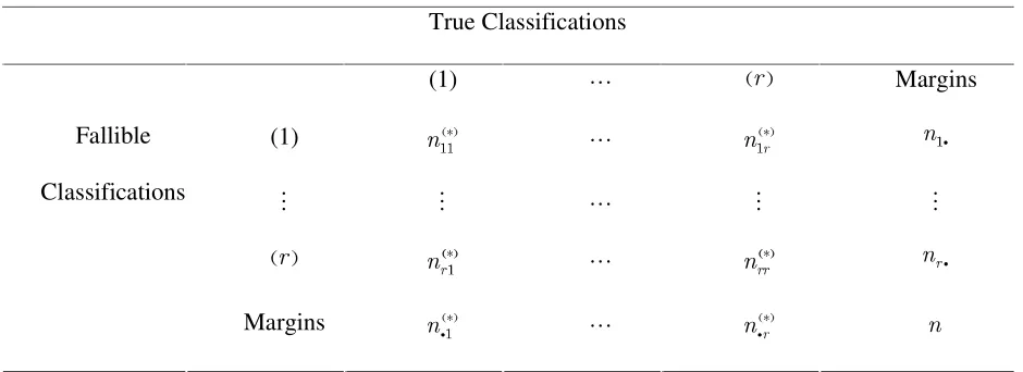
observed with the true classifications (Tables 1 and 2). Using a subscript

( )

∗ to denote unobserved

quantities, denote by IKJ LM NN

, IGJ

O

LM

N the counts referring to this cross-classification in the main sample and

in the validation sample respectively. Denote also by PKQRPQ S T T NU N

V V the total number of sample units classified in state K by the “perfect” classifier in the main sample and in the validation sample

[image:8.612.80.550.333.502.2]

respectively.

Table 1: Data from Validation sample

True Classifications

(1) _" W X

R _Margins

(1) PGQ

YZY

S

N _" [\

]^ _

N [G\

]^ N`

# # " # #

W X

R acb

d

e

f

N _" acb

e

ff

N [G\

^

_

N ` Fallible

Classifications

Margins gGh

ij

Nk "

lm

n

o

Np

qGr

s

N

Table 2: Data from Main sample

True Classifications

(1) _" W X

R Margins

(1) [K\

]Z]

Nt " [K\

]_

Nu v

Nw

# # " # #

W X

R lKm

i

o

Nx "

lKm oo

Ny z

N { Fallible

Classifications

Margins [K\

]

Nu

| "

[K\

_

Nu

[image:8.612.81.551.542.713.2]

The key concept of the above parameterisation is that both the main sample and the validation

sample have a similar structure as this is described in Tables 1 and 2. However, for the validation

sample full information exists while for the main sample we have only marginal information about the

observed classifications. The idea is to formulate a model by combining information from the main

sample and from the validation sample. The basic assumption is that these two samples share

common parameters because both are assumed to be representative of the same population. This

parameterisation will lead to an optimisation problem that involves missing data. This is due to the

fact that the validation procedure is not applied to the units of the main sample. Assuming

independence between the main and the validation sample, denoting by ~=

€

$ the complete data and by

2 the vector of parameters, the full data likelihood is given by

K‚

ƒ…„

ƒ†„

‡ˆ‡ ‡ˆ‡

‰

Š‹ Š‹

ŒŒ ŒŒ

Ž Ž

 ’‘ ’‘

‘“ ‘R

, $ 0 Q 0 Q

”

•ˆ• •ˆ•

2

_

_

(3.1)

Taking the logarithms in both sides of (3.1) and imposing the additional constraints that

–

—

˜

˜

0

™

œ

(3.2)

š ÅFORÅFIXEDÅK

›

œ

œ

Q

ž

œ

(3.3)

we obtain the following expression for the full data log-likelihood

Ÿ¡ 

Ÿ¢  Ÿc 

Ÿ¢  Ÿ¢ 

Ÿc  Ÿ¢ 

Ÿc  Ÿ¡ 

£ £ £

£R£ £ £

£

£

LOG LOG LOG

ÅÅÅÅÅÅÅÅÅÅÅÅÅ LOG

¤¥¤ ¤ ¤

¦ § § §

¨© ¨© ¨©

¤

©

¤

© ¨© © © ©

©ª¨ ¨ ©

¤

§

¤ ¤

©

©

L $ N N Q N N Q N N 0

N N 0

« « «

¬ ¬ ¬

­R­ ­ ­

«

¬

­

¯

 _¬­

ž

  °

2 _¢ ž ­_­­°

žŸ _®±

 _¬­

ž

ž ­_­­

žŸ ®

œœ

œ

œ

œ

® ®

® ®

(3.4)

The log-likelihood function (3.4) contains unobserved data. One way of using this likelihood to

maximise the likelihood of the observed data is via the EM algorithm (Dempster, Laird and Rubin

1977). The EM algorithm is based on two steps, namely the expectation (E-step) and the maximisation

(M-step). Generally speaking, the algorithm is initialised using a set of arbitrarily selected starting

statistics defined by the complete data likelihood (e.g. equation (3.4)) are replaced by their conditional

expectations given the observed data and the current set of parameter estimates. Having computed

these conditional expectations, the full data likelihood is maximised to produce a new set of maximum

likelihood estimates. Using this new set of maximum likelihood estimates, new conditional

expectations are computed in the E-step and new maximum likelihood estimates are derived in the

M-step. The E and M step are iterated until a convergence criterion is satisfied. For the currently

described model these steps are described below.

We start by taking the conditional expectation of the full data log-likelihood given the observed

data and the current estimates. We denote by ¯°

±

$ the data derived from the validation sample, by

²´³

µ

$ the data derived from the main sample and by H the current EM iteration. The form of the full data log-likelihood after taking the conditional expectations becomes

¶¡·

¶c·ˆ¶¸·¹=º ¶¡· ¶c·

¶¸·ˆ¶c·»¹=º

¶¡· ¶c·

¶¸·ˆ¶c·»¹=º ¶c· ¶¡·

¶·ª¶c·»¹Kº

¶c· ¶¢·

¶¸·ˆ¶c·»¹=º ¼ ¼½¼ ¼ ¼ ¼ ¼

\ \ LOG

ÅÅÅÅÅ \ LOG \ LOG

ÅÅÅÅÅ \ LO

¾¿¾

À À

Á Â Ã Â Ã Â

ÄÅ ÄÅ ÄÅ

ÅÆÄ

¾ ¾

À À

 à   à Â

¾

Å

¾

Å ÄÅ Å Å Å

Ä Å

À

 à Â

¾ ¾

% L $ $ $ % N N $ $ Q

% N N $ $ Q % N N $ $ 0

% N N $ $

Ç È ÉÊÉ Ç Ç È È É É È  

  _{2 2} ¯   ₂ ¯

¡ ° ¡ ¡ °

¢ ± ¢ ¢ ±

¯

 _¬­

ž

  2 ¯ ž ­°   2 ¯

¡ ° ­ ¡ °

¢ ± _žŸ ­_®±° ¢ ±

  ₂ ¯

¡ °

¢ ±

œœ

œ

œ

Ë Ë

Ë Ë ¼ ¼ G ¾ Å Å 0 Ç É  _¬­ ž ­ ž _­­ žŸ

œ

® (3.5)

Under this parameterisation, unobserved quantities exist only in the main sample. The expectation

step (E-step) and the maximisation step (M-step) can be performed using the following two results.

Result 3.1

For the E-step, the conditional expectations of the missing data in the main sample are estimated using

the following expressions

ÌKÍ ÌÎÍ ÏÑÐ

ÏÒÐ ÏÑÐ ÏÑÐ ÏÑÐ Ó \ Ô Ô Õ Ô Ö × Õ Ø × Õ × Ô Ô Õ × Õ Õ 0 Q

% N $ N

0 Q Ù Ù Ù Ú Ù Ù Û   ¯ ¡ ° ¡ °

2 ¡ °

¡ °

¡ °

¡ °

¢

œ

±

Ü and

ÝKÞ Ý´Þ ßÑà

ÝKÞ ßÑà

á \ \ â ã ã ä ä

å æå

æ

% N $ % N $

ç ç

è è

é

2

_œ

2

ê (3.6)

Proof

Result 3.2

For the M-step, the maximum likelihood estimators are given by the following expressions

ëKì ëÎìîíÑï

ëì

ëKì ëÎì íÑï

ëì

\ \

ð

ñ ò

óô óô

óô

ð

ñ ò

ô ô

% N $ N

Q

% N $ N

õ ö

õ

õ ö

2

2

÷ ÷

and

øKù ø´ùûúÑü

øù

øGù ø´ù úÑü

øù

ý

\

\

þ

ÿ

þ

ÿ

% N $ N

0

% N $ N

2

2

œ

(3.7)

Proof

Proof of Result 3.2 is given in Appendix A.

Identification of the model parameters can be checked by initialising the EM algorithm from

different starting values and seeing whether the algorithm converges to the same solution. We assume

that convergence is achieved when the difference between the maximum likelihood estimates obtained

from two successive iterations of the EM algorithm, as this is measured for example by the

, norm, is less than a small value E.

Independence between the main and the validation sample is not guaranteed only under a double

sampling scheme where the validation sample is selected independently from the main sample.

Alternatively, one can select a validation sample by sub-sampling

N units from the main sample and

then form two samples i.e. one in which the sampled units participate only in the main survey and

another in which the sampled units participate both in the main and in the validation survey.

As we will later illustrate, in a cross-sectional framework the parameterisation of the

misclassification model using the calibration probabilities (Section 2.2) or the misclassification

probabilities (current section) will lead to identical results. However, in some cases the use of the

misclassification probabilities is more reasonable than the use of the calibration probabilities. Such a

case, where the standard measurement device is a panel survey and a cross-sectional validation survey

is used, is presented in Singh and Rao (1995). Due to the cross-sectional nature of the validation data

that are used in this paper, a conditional independence assumption is employed in order the parameters

of the longitudinal misclassification mechanism to be identified. More specifically, the authors assume

true states. It has been proven by Meyer (1988) that this assumption should be used only in

conjunction with the misclassification and not with the calibration probabilities. Therefore, the

formulation of the misclassification model using the misclassification probabilities offers a robust

basis for extending the model to handle more complex situations.

3.2 Variance Estimation for the Maximum Likelihood Adjusted Estimates

Variance estimation for the maximum likelihood adjusted estimates can be placed into the general

framework of maximum likelihood estimation. This implies the use of the inverse of the information

matrix. However, due to the formulation of the misclassification model as a missing data problem, the

variance estimates should account for the additional variability introduced by the existence of missing

data in the main sample. One way to perform variance estimation in an EM framework is by applying

the Missing Information Principle (Louis 1982).

Denote by

2 the vector of maximum likelihood estimates and by

: : the missing data in the

main and in the validation sample respectively. The missing data and the observed data

$ $

define the complete data

$ . The Missing Information Principle is defined as

/BSERVED Å)NFORMATIONÅÅ#OMPLETEÅ)NFORMATION-ISSINGÅ)NFORMATION (3.8)

Lemma 3.1 (Louis 1982)

The complete information is evaluated at

2 using the following expression

Å \ ! "

#

L $

#OMPLETE )NFORMATION % ¡_¡s 2 $ $ ¯°_°

s2s2

¢ ±

(3.9)

Lemma 3.2 (Louis 1982)

The missing information is evaluated at

2 using the following expression

$%

$%$%

\

&

' (

L $

Å-ISSINGÅ)NFORMATION 6AR ¡_¡s 2 $ $ ¯°_°

s2

¢ ±

Lemma 3.3

Conditionally on the information in the main sample, there are R multinomial distributions defined by the R rows of the cross-classification of the observed with the true classifications (see for example Table 2).

Proof

Proof of Lemma 3.3 is given in Appendix A.

The evaluation of the expectation of the complete information matrix involves the second order

derivatives of the log-likelihood function with respect to the vector of parameters. The evaluation of

the covariance matrix of the score functions involves the first order derivatives of the log-likelihood

function with respect to the vector of parameters. Under simple random sampling, the variance of the

score functions can be computed using Lemma 3.3 and standard results for the variance of a sum of

binomial random variables. However, even for the -state misclassification model, the evaluation of

the elements of this covariance matrix is tedious. Instead, we can approximate the components of the

Missing Information Principle using a simulation-based procedure. Having arrived at the maximum

likelihood estimator, we generate (complete data sets (main samples) by drawing

)*)* )* )* )*

+ , \

--.

/ / / / /

0

: : : P : $

1

2

! (3.11)

where 23 23

\ 4 4

P : $

5

2 denotes the conditional distribution of the missing data in the main sample

given the observed data and the maximum likelihood estimates and ( denotes the total number of

simulations. This conditional distribution is defined by Lemma 3.3. This first step of the simulation can

be viewed as the imputation step. Having replaced the missing data with imputed values in simulation

H , we derive complete data 6879 :

;=<

$ that are employed for evaluating the complete information matrix

and the missing information matrix. This is done by using the simulation-based (empirical) estimators

for the complete information matrix and for the variance of the score functions over simulations

>8?

>?>?

>?@BA

C

C

D

\

Å Å

EGF

E H

I J

K K

F

L $

L $

% $ $

( L

  _{s 2} ¯ s 2

¡ °

¡ _{s2 s2} ° _{s2 s2}

¢ ±

œ

(3.12)

MN

MNMN

MNOBP

M8NOBP

Q

R

\

S=T S=T

S U

V W

T

L $ L $

L $

6AR $ $ %

( X

£   ¯²

¦ ¦

 s 2 ¯ ¦_¦s 2 _¡s 2 _°¦_¦

¡ _{° ¤ ¡ °»}

¡ _s2 ° _{¦ s2 ¡ s2 °¦}

¦ ¦

¢ ±

œ

_{¦¥ ¢ ±¦¼}

(3.13)

Having evaluated the complete information matrix and the missing information matrix, the

covariance matrix of

Y

2 is then determined by the inverse of the matrix defined by the difference of these two matrices

Z8[

Z[Z[

Z8[

Z[Z[

\

]

\ \

Å

^ ^

_ ` _ `

a

L $ L $

6AR % $ $ 6AR $ $

b

c £   ¯   ¯²

¦ s 2 s 2 ¦

¦ _{¡ ° ¡ °}¦

2 ¤ _{¡ ° ¡ °}»

¦ s2 s2 s2 ¦

¦ ¢ ± ¢ ±¦

¥ ¼

(3.14)

4. A QUASI-LIKELIHOOD PARAMETERISATION OF THE MISCLASSIFICATION MODEL

In this section we present a quasi-likelihood parameterisation of the misclassification model. This

parameterisation offers an alternative to the EM algorithm way of resolving a missing data problem.

The advantage of this approach is that it does not require any explicit definition of the likelihood

function.

The approach we follow was introduced by Wedderburn (1974) as a basis for fitting generalised

linear regression models. As described in Heyde (1997), Wedderburn observed that from a

computational point of view the only assumptions for fitting such a model are the specification of the

mean and of the relationship between the mean and the variance and not necessarily a fully specified

likelihood. Under this approach, Wedderburn replaced the assumptions about the underlying

probability distribution by assumptions based solely on the mean variance relationship leading to an

estimating function with properties similar to those of the derivative of a log-likelihood. This

estimating function is usually referred to as the quasi-score estimating function. The quasi-likelihood

estimator is then defined as the solution of the system of equations defined by the quasi-score

estimating function. To illustrate, consider the following model

where 9 is a Nq data vector and %dfeF . The quasi-score estimating function ' 2 is then

defined (Heyde 1997 Theorem 2.3) as

gih < >

j

k

' sN 2 ­¬ 6AR F l F ž

2 ž_žŸ ­_­­®

s2 (4.2)

The quasi-score estimating function defined by (4.2) is also referred in the literature as

Wedderburn’s quasi-score estimating function.

4.1 The Model

Denote by mon

p

q

0 the probability of correct classification in category K for units in the validation

sample, by rs

t

uv

Q the probability of misclassification for units in the validation sample, by Nwx the

number of units in the main survey classified in category I by the standard measurement device and by

N the sample size of the main survey. Without loss of generality, we describe the model for the case of

two mutually exclusive states to which a sample unit can be classified. Instead of specifying the form

of the likelihood function, the model can now be described by a system of equations. The number of

equations we need is defined by the smallest possible set of independent estimating equations that can

be established for the underlying problem. For the two-state cross-sectional misclassification model

one possible system of equations is

yz

yz yz

{

{ { {|{ {|{ } {~} {~} 

{ {{|{ {€{~} 

‚

‚

‚

0 0

Q Q

Q Q

N N 0Q 0 Q

F F F

F

ƒ

ƒ

ƒ

²¦

_¦¦

¦¦ ¦

_¦¦¦

» ¦¦

_¦¦

¦¦

  ¯

_{¢ ±} ¦_¦¦¼

„

(4.3)

Note that N… N PR 9

†

‡ ˆ

‰ . The left hand side of the equations given in (4.3) describes estimates obtained from the main and the validation sample whereas the right hand side describes the unknown

parameters of interest plus an error term. Equations described by (4.3) incorporate the extra constraints

Š ‹

0 0,QŒŽ Q and QŒŒ Q~Œ . Likewise in a maximum likelihood framework, in a quasi

likelihood framework we assume that the main and the validation sample share common parameters

due to the fact that both are representative of the same population.

Assuming the general form of the model defined by (4.1), denote by F the vector of errors, by

N 2 the vector of means and by 2 0 Q‘|‘“’ Q

the vector of parameters. Following Heyde (1997),

Wedderburn’s quasi-score estimating function is then defined as

”i• < >

–

—

' sN 2 ­¬ 6AR F ˜ F ž

2 ž_žŸ ­_­­®

s2 (4.4)

Equation (4.4) for the two-state model can be expressed as follows

™š ™›š ™š œ  œ œ œ œ“ œ“ž œ Ÿ  œœ œ“ œ  |ž ~Ÿ œœ œ|œ œ  ž¡œ ž ž ž|Ÿ œ| œ| œ  ŸŽœ Ÿ¡ Ÿž Ÿ œ œœ|œ œ¢œ“ ÅÅ £ £ £ 0 0

N Q Q

Q Q

' N 0

Q Q

N 0

N N 0 Q 0 Q

T T T T T T T T T T T T T T T T

¤ ¥ ¤ ¤ ¤   ¬_­ ž_ž ž _­  ¬_­ž_{ž ­} ž_ž ž _{­ ž ­} ž ­ž ­ ž _{­ ž} ­ ž _{­ ž} ­_­ ž

2 _ž ­_{­ž ­}

­ ž ž ­_{­ž ­} ž _{­ ž ­} ž ­­ ­ ž ž ž ­ Ÿ _{®­ ž ­­} žž ­   ¯ Ÿ ®­ ž _Ÿ ¦ _{¢ ±} ¬­ ­­ ­­ ž ­ ž ­ ž _­­ ž _­ ž _­ ž _­ ž ­ ž ­ ž ­ ž _­­ ž _­ ž ­ ž _­® ž _­ (4.5)

Setting (4.5) equal to zero then leads to three quasi-score normal equations. These equations need to be

solved using numerical techniques.

In the system of quasi-score normal equations defined by (4.5), the elements of the covariance

matrix of the error terms are unknown and need to be estimated using the sample data.

Under simple random sampling (i.e. assuming a multinomial distribution), §

¨

T , §

©

T can be estimated by ª« ª«

ª«

¬ ¬ ­ ¬ ­® ¯ ¯ ¯ 0 0 N

N PR 9° PR 9°

T T ± ± ± ± ± ± ² ² ²¦ ¦ ¦¦ ¦¦_» ¦¦ ¦   ¯ _{¡¢ ° ¦}¦ ± ¦¼ (4.6)

In order to estimate the covariance matrix of the estimates of the misclassification probabilities, we

denote by ³´

µ

¶·

N the number of sample units in the validation sample classified by the standard

probabilities are denoted by ¸¹ º » ¼½ ¾ ¼½ » ¼½ ¼ N Q N ¿ À

œ

and the estimated matrix of misclassification probabilities

by 1

Á

. While Âoà Âà ÄÅÄ ÆÇÆ È È ÉÊ ÉËÊ N N ÌÅÌ

œ œ

can be considered as fixed, ÍoÎ

Ï Ð Ñ ÒÓ Ò N Ô

œ

must be considered as random.

Consequently, in the computation of this covariance matrix we must take into account the non-linearity

introduced by the fact that both the numerator and the de-numerator of QÕÖ

×

are random quantities.

Therefore, we apply the Delta method (Bishop, Fienberg and Holland 1975). Let

ØÙÚØÙÚØÙÚØÙ

Û|ÛÜ¡ÛÝÛ~ÜÞÜ|Ü ß ß ß ß

N N N N

à

á

2 and â

ã ã ã

ä

å

æ

VEC 1 F F

ç ç ç

  _ž ¬_­¯   _ž ¬_­ _ž ¬_­¯ ¡ _žž2 _­­° ¡ _žž2 ­_{­ žž}2 _­­° ¡ Ÿ ®° ¡ Ÿ ® Ÿ ®°

¢ ± ¢ ± be an

è

R q vector of functions of

é

ê

2 . Applying the delta method to

ë

VEC 1

ì

  _{ž ¬­}¯ ¡ _{ž2 ­­}°

ž ¡ Ÿ ®° ¢ ±

we obtain the following approximation

í í

í î î î î

ÅÅ \ ÅÅ

Å

VEC 1

VEC 1 VEC 1 ï

ð

ñ

ò ò

ñ ó ó

ó ô ó   ¯ s 2  ¬

  ₂ ¯   _{2 ¯ x ‹ ž2 2 ­ ‹} ¡_¢ °_± ¡ ° ¢ ± ž_žŸ ­­_®

¡ ° s2

¢ ± (4.7)

Taking the variance operator on both sides of (4.7) leads to

<

>

õ õ

ö

÷

6AR VEC 1 6AR

ø

ù ù

 _¬­ ž

x ‹ ž_{žŸ ®}2 ­_­ ‹ (4.8)

Under simple random sampling,

ú 6AR û  _¬­ ž2 ­ ž _­

žŸ ® can be estimated using the following results

üý

üý

üýÚüý

þÿþ ÅÅ

6AR N N PR 9 I 9 K PR 9 I 9 K

#OV N N N PR 9 I 9 K PR 9 I 9 K I K I K

£¦   ¯ ¦ _{¡ °} ¦ ¢ ± ¦¤

¦¦ v

¦¦¥

(4.9)

Substituting (4.9) and the Jacobian matrix into (4.8) we obtain estimates for T ,T and

T T .

For estimating the covariance terms TT T we need to consider the double sampling scheme

that we employ. In Section 3.1, we mentioned that independence between the main and the validation

sample can be assumed both when the validation sample is selected independently from the main

for the former case this argument is clear, for the latter case more explanation is required. More

specifically, for the latter case independence is guaranteed by splitting the sample into sample units

that participate only in the main survey and sample units that participate both in the main and in the

validation survey. Under the assumption of independence between the main and the validation sample,

the following holds

T T T T T T (4.10)

It only remains to estimate the following covariance terms: T T and T T . These

covariance terms can be more generally defined as follows

"! #!

#! "! #! #! $ $ % & '( & & & '( ' ( % '( & & '( ' N N

#OV Q 0 #OV

N N ) ) * *  _¬­ ž _­ ž _­ ž _­ ž ­ _{ž ­} ž ­ ž _­­ ž _­­ žžŸ ®

œ

œ

(4.11)

Estimation of these covariance terms is performed using the results below.

Lemma 4.1(Mood et.al. 1963)

An approximate expression for the expectation of a function G 8 9 of two random variables 8 9 using a Taylor’s series expansion around N N+-,

is given by

<

>

. . / / . . . / \ \

\ ÅÅ

021 021

031 465

% G 8 9 G G 8 9 6AR 9 G 8 9 6AR 8

Y X

G 8 9 #OV 8 9 X Y

727 727

727

N N s s

x s s s s s (4.12) Result 4.1

Assume that 8 9 ! are three random variables and N is fixed. A first order approximation for

8 ! #OV 9 N  _¬­ ž _­ ž _­

žŸ ® is given by

% 8 8 !

#OV #OV ! 8 #OV ! 9

9 N N% 9 % 9

  ¯

 _{¬­ ¡ °}

ž _­x

ž _­

ž ¡ °

Ÿ ® _{¢ ±} (4.13)

Proof

Setting 8#9 8"9 8#9

: :

Å Å

< < < => => =>

= =

8 N 9 N ! N

? ?

_œ

_œ

and @

N N in Result 4.1, we can then estimate the

remaining covariance terms of interest.

Having obtained estimates for the variance terms, the final step in deriving the quasi- likelihood

estimators is to solve the system of equations defined by (4.5). This can be done using a

Newton-Raphson algorithm. Define by 2 the vector of parameters of dimension Xq, and by ! a XqX

matrix with elements A Å AB

B

'

! I J X

+ s 2

s " . The system of quasi-score normal equations

defined by (4.5) can be now solved numerically as follows. Assume a vector of initial solutions CED

F

2 . The vector of initial solutions can be updated using

GIH JLK JLK JLK

M N N N

M

! '

O O O O

P   ¯   ¯ 2 2 ¡2 ° ¡2 ° ¡ ° ¡ °

¢ ± ¢ ± (4.14) The iterations continue until a pre-specified convergence criterion is satisfied.

4.2 Variance Estimation for the Quasi-likelihood Adjusted Estimates

Variance estimation for the quasi-likelihood adjusted estimates is performed using the following

result.

Result 4.2

The variance of the quasi-likelihood adjusted estimates is estimated using the expression below

QSR

T

T

\ \

U

6AR N V 6AR F N V

W

W

X X X

Y[Z\Y Y[Z]Y

£ ²

¦s 2 ¬   _¯ s 2 ¬¦ ¦ž ­ ž ­¦ 2 x¤_¦ž_{Ÿž s2} ­_{® ¢­­} ¡ °_{± Ÿž}ž _{s2 ­­®}­_¦»

¦ ¦

¥ ¼

(4.15)

Proof

Proof of this result is given in Appendix B.

Although some work is required in order to derive 6AR^`_F

a

, the evaluation of the covariance matrix

of the quasi-likelihood estimates is straightforward since it requires the utilization of matrix quantities

EM context that requires the use of computer intensive techniques, variance estimation under the

quasi-likelihood parameterisation may be more appealing to the data analyst.

5. APPLICATIONS

5.1 Application 1

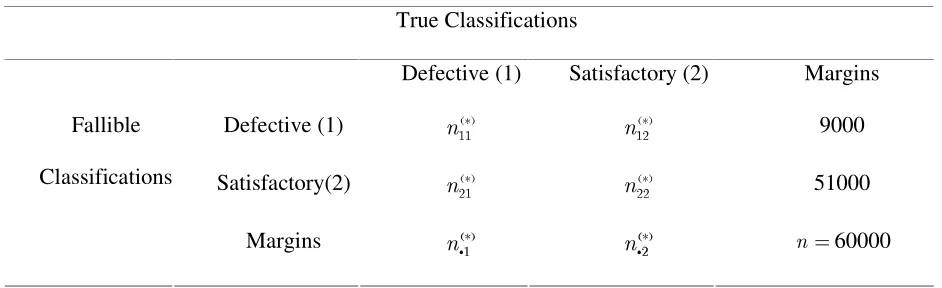
The alternative approaches are illustrated using the following numerical example.A firm wishes to

assess the quality of the units that it produces. The units can be classified into two categories:

Defective (1) or Satisfactory (2). There are two classification methods. One, which is currently used, is

inexepnsive and is subject to measurement error. Altenatively, the firm can use an accurate but more

expensive classification method. The firm suspects that a number of truly satisfactory units are

classified as defective. The management team is interested in investigating the trade-off between the

loss of satisfactory units and the extra cost of improving the currently used classifier. A sample of

N production units is selected and the units are classified using the inexpensive classification method. In order to validate the inexpensive classifier, another sample of b#c

d

N production units is selected and these units are classified using both the expensive and the inexpensive classifier.

The data for this numerical example are given in Tables 3 and 4. The estimators we consider are the

undajusted for misclassification estimator (Naïve), the maximum likelihood estimator (MLE) with

callibration probabilities (Section 2.2), the maximum likelihood estimator (MLE) with

misclassification probabilities (Section 3.1) and the quasi-likelihood estimator (Section 4.1).

Table 3: Data from the Validation Sample Used in Application 5.1 True Classifications

Defective (1) Satisfactory (2) Margins

Defective (1) 672 918 1590

Satisfactory (2) 28 8382 8410

Fallible

Classifications

Margins 700 9300 e#f

g

[image:21.612.80.551.84.228.2]

Table 4: Data from the Main Sample Used in Application 5.1 True Classifications

Defective (1) Satisfactory (2) Margins

Defective (1) hji kk

Nl mjn

op

Nq 9000

Satisfactory(2) mjn po

Nq mjn

pp

Nq 51000

Fallible

Classifications

Margins rjs

t

Nvu

wjx

y

N{z N60000

Table 5: Proportion of Units Classified as Defective Under the Alternative Parameterisations of the Misclassification Model, Standard Deviations in Parentheses

Point Estimator Proportion of Units Classified as Defective

Naïve (Unadjusted Estimator) 0.1512 (1.35*10-3 ₎

MLE (Calibration Probabilities) 0.0667 (2.08*10-3₎

MLE (Misclassification Probabilities) 0.0667 (2.07*10-3₎

Quasi-likelihood 0.0669 (2.11*10-3)

The convergence criterion for the EM algorithm and for the Newton-Raphson is E} | . An

empirical investigation of the identifiability of the model parameters is provided by initialising the EM

and the Newton-Raphson algorithms using different sets of starting values and checking whether these

algorithms converge to the same value.Using this diagnostic, we conclude that the model parameters

are identified. All three estimators that correct for measurement error produce similar results. The

management team of the firm can now decide whether it worths investing in improving the

inexpensive classification procedure. The variance of the naïve (unadjusted) estimator is computed

under simple random sampling assuming a multinomial distribution. The variance of the maximum

likelihood estimator that employs the calibration probabilities is computed using the result of

and of the quasi-likelihood estimator is computed using the results from Sections 3.2 and 4.2

respectively.

Assuming that the validation survey provides an unbiased estimate of the proportion of units that

are trully classified as Defective, we can then examine the efficiency of the alternative estimators.

Although the estimators that account for measurement error have higher variances than the estimator

that ignores measurement error, they are unbiased. On the other hand, the estimator that ignores

measurement error is seriously biased. Therefore, in mean squared error terms, we conclude that

accounting for measurement error will produce more efficient estimates than ignoring measurement

error.

5.2 Application 2: Contratsing the Alternative Parameterisations in the Presence of Intense

Misclassification

In Section 2.1 we mentioned that in the presence of intense misclassification the moment-based

estimator can produce estimates that lie outside the parameter space. We now utilise a numerical

example for comparing the alternative parameterisations when intense misclassification exists. A

sample of N units is selected and the units are classified into two mutually exclusive categories, denoted by (1) and (2), using an inexpensive classification method. In order to validate the

inexpensive classifier, another sample of ~"

€

N units is selected and these units are classified using both the expensive and the inexpensive classifier. The data for this numerical example are given

in Tables 6 and 7. The estimators we consider are the moment-based estimator (Section 2.1), the

maximum likelihood estimator (MLE) with callibration probabilities (Section 2.2), the maximum

likelihood estimator (MLE) with misclassification probabilities (Section 3.1) and the quasi-likelihood

[image:23.612.90.548.439.568.2]

Table 6: Data from the Validation Sample Used in Application 5.2 True Classifications

(1) (2) Margins

(1) 500 4400 4900

(2) 500 14600 15100

Fallible

Classifications

Margins 1000 19000 #‚

ƒ

N 20000

Table 7: Data from the Main Sample Used in Application 5.2 True Classifications

(1) (2) Margins

(1) N††„j…

‡ ˆj‰

Š‹

NΠ13600

(2) ˆj‰

‹Š

NŒ ˆj‰ ‹‹

NΠ46400

Fallible

Classifications

Margins jŽ



N‘ ’j“

”

N–• N60000

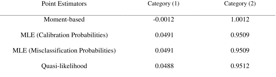
Table 8: Adjusted Proportion of Units Classified in Each Category Under the Alternative Parameterisations of the Misclassification Model

Point Estimators Category (1) Category (2)

Moment-based -0.0012 1.0012

MLE (Calibration Probabilities) 0.0491 0.9509

MLE (Misclassification Probabilities) 0.0491 0.9509

Quasi-likelihood 0.0488 0.9512

The intensity of the misclassification problem can be seen by noticing that 50% of the units that

truly belong in category (1) are misclassified as being in category (2) (see Table 6). The results (Table

8) indicate that when high misclassification exists, the moment-based estimator can lead to ackward

estimates (in this case negative proportions). On the other hand, both the maximum likelihood

6. SIMULATION STUDY

6.1 Design and Implementation of the Simulation Algorithm

The alternative parameterisations are empirically compared using a Monte-Carlo simulation study.

The simulation algorithm simulates the measurement error process in a double sampling framework.

The algorithm involves four steps. At the first step we generate true classifications for each sample

unit Y. This is done by assuming the probability distribution function of the true classifications. Using

this distribution, we draw a with replacement sample of size N . The probabilities of correct

classification that we use are PR 9—

and PR 9˜

. At the second step we

assume the existence of measurement error that is described by the misclassification probabilities Q™š .

Using these misclassification probabilities, we generate the observed status, given the true status (Step

1), for each sample unit Y. The diagonal elements of the misclassification matrix that we employ are

››

Q and Qœœ . According to the methodology that assumes the availability of validation information the estimation of the matrix of misclassification probabilities is based on the validation

sample. We simulate a validation sample by selecting a with replacement sample of #ž

Ÿ

N independently from the main sample and from the same target population. The probability structure of

 

PR 9¡ I 9¡ K is defined as follows:

¢

Å

PR 9£ 9£

¤

PR 9¥ 9¥

¦

PR 9§ 9§

¦

ÅPR 9§ 9§ The first three steps summarise the

generation process. At the final step we employ the generated data for computing the alternative

estimators. We conduct a total of ( simulations and we empirically evaluate the properties of the alternative point estimators (averages over simulations) using (a) the bias of a point estimator, (b)

6.2 Results

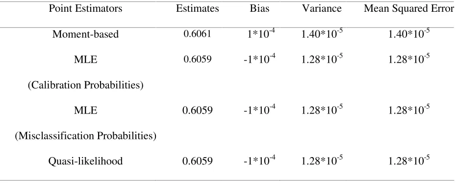
The results from the Monte-Carlo simulation are summarised in Table 9.

Table 9: Monte-Carlo Simulation Results for Comparing the Alternative Parameterisations of the Misclassification Model

Point Estimators Estimates Bias Variance Mean Squared Error

Moment-based 0.6061 1*10-4 _1.40*10-5 _1.40*10-5

MLE

(Calibration Probabilities)

0.6059 -1*10-4 _1.28*10-5 _1.28*10-5

MLE

(Misclassification Probabilities)

0.6059 -1*10-4 _1.28*10-5 _1.28*10-5

Quasi-likelihood 0.6059 -1*10-4 1.28*10-5 1.28*10-5

7. DISCUSSION

Two alternative parameterisations for maximum likelihood estimation using either the calibration

or the misclassification probabilities are presented. In a cross-sectional framework, both

parameterisations for maximum likelihood estimation lead to identical results. However, it has been

shown (Mayer 1988) that the use of misclassification probabilities instead of the calibration

probabilities is more reasonable when handling more complex situations for example, when analysing

longitudinal misclassified data. Thus, we suggest that the parameterisation of the misclassification

model as a missing data problem using the misclassification probabilities provides a more general

method and it should be preferred.

As an alternative approach, we further presented a quasi-likelihood parameterisation of the

misclassification model. This approach offers an alternative to the EM algorithm way of resolving a

missing data problem, which at the same time does not require full specification of the likelihood

function. The results from the simulation study show that the quasi-likelihood estimator is as efficient

[image:25.612.84.551.157.344.2]

offers is an easier way of performing variance estimation for the adjusted estimates. More specifically,

variance estimation for the maximum likelihood estimator when using the EM framework involves the

application of the Missing Information Principle and may require the use of computer intensive

methods. On the other hand, variance estimation in a quasi-likelihood framework is much simpler and

requires the utilization of matrix quantities that have been already used during the estimation process.

In section 2.1, we reviewed a moment-based estimator and mentioned that one of the main

disadvantages associated with the use of this estimator is that it can produce estimates that lie outside

the parameter space for example, negative adjusted estimates. Unlike the moment-based estimator,

both the maximum likelihood estimators and the quasi-likelihood estimator constrain the derived

estimates to lie within the boundaries of the parameter space. Moreover, the simulation study verifies

the superiority of the maximum likelihood and the quasi-likelihood estimators when compared to the

moment-based estimator.

Currently, we investigate the extension of the quasi-likelihood approach for analysing longitudinal

misclassified data. We also examine ideas for applying the misclassification model in other areas of

statistical inference. For example, in demographic applications one of the most commonly encountered

problems is heaping. A traditional way of resolving this problem is via the use smoothing techniques.

An alternative solution can be offered by viewing heaping as a misclassification problem. A further

possible application is in statistical disclosure control. More specifically, one way of protecting the

data is by misclassifying them and providing to the data analyst the misclassified data along with the

misclassification probabilities (Van den Hout and Van der Heijden 2002). The basic difference

between the approach utilised in statistical disclosure control and our approach is that in the former

case the misclassification probabilities are treated as fixed whereas in the latter case the

misclassification probabilities are random since they are estimated from the validation survey. Finally,

another application regards adjustments in the Census. For example, the existence of inaccurate

described in a misclassification context and a model that combines information from the Census (main

survey) and from a post-enumeration survey (validation survey) can provide adjustments to the

Census-based estimates.

APPENDIX A: PROOFS OF THE RESULTS IN SECTION 3

Proof of Result 3.1

The number of sample units that belong in the IK cell of the cross-classification of the observed by

the true classification is denoted by ¨j© ª«

N¬ . Note that while a superscript ­® refers to the unobserved quantities, a superscript refers to the observed classifications. The expectation of an unobserved

quantity is given by

¯j°

±²

% N N% 9³ I 9³ K

´ ´

(A.1)

Equation (A.1) can be re-expressed as follows

µj¶

\

·¸

% N N% 9¹ I 9¹ K % 9¹ K

º º

(A.2)

From the main sample we have information about the observed classifications N»¼ .

½

\

¾

¿ À

N N % 9Á I 9Á K % 9Á K

Â

Ã

_œ

Ä (A.3)

Given the data constraints N»

¼, the conditional expectations of the unobserved quantities are given below

ÅjÆ ÅÇÆ

È

\

\

\

É

Ê Ë

ÌÍ Ì

Í

% 9 I 9 K % 9 K % N $ N

% 9 I 9 K % 9 K

Î Î Î

Î Î Î

Ï

Ï

Ï

Ð

  ¯

¡ °

¡ °

¡ °

¡ °

¡ °

¡ °

¢

œ

±

Ñ (A.4)

The expectations of the random variables involved in the expression above can be computed using

well known results for binomial random variables. More specifically,

PR 9 I 9\ K

QÒÓ

Ô Ô

Õ

, PR 9× K

0Ö (A.5)

ØjÙ ØÇÙ ÚÜÛ

ÚÜÛ ÚÜÛ ÚÜÛ ÚÜÛ Ý \ Þ Þ ß Þ à á ß â á ß á Þ Þ ß á ß ß 0 Q

% N $ N

0 Q ã ã ã ä ã ã å   ¯ ¡ ° ¡ ° 2 ¡ ° ¡ ° ¡ ° ¡ ° ¢

œ

±

æ

It follows that

çjè çéè êÜë

çjè çÇè êÜë

ì \ \ í î î ï ï

ð ñð

ñ

% N $ % N $

ò ò

ó ó

ô

2

œ

2

õ

Proof of Result 3.2

The system of normal equations that we need to solve in order to obtain the maximum likelihood

estimators is defined by setting the score functions equal to zero i.e.

öÇ÷6ö#÷

\ ø ù úû

% L $ $ Q

s 2

s (A.6)

The ü

ü

R R q R R system of normal equations and the corresponding maximum likelihood

estimator for Qýþ is given below.

ÿ ÿ

ÿ ÿ ÿ

ÿ

ÿ ÿ

ÿ ÿ ÿ

ÿ

\ \ \ \

% N $ N % N $ N

Q Q Q

% N $ N % N $ N

Q Q Q

²¦

2 2 _¦¦

_{¦¦ ¦¦} ¦¦¦ » ¦¦ ¦¦

2 2

¦¦ _{¦ ¦¦¼¦} " # " (A.7)

\ \

% N $ N

Q

% N $ N

2 2 (A.8)

Similarly, for0 , the R q R system of normal equations and the corresponding maximum

likelihood estimator is given by the following expressions

! !"#

! ! !"#

!

! ! "#

! ! ! "#

!

$ $ $ $ $ $ $ $ $ $ \ \ \ \ % %

& ' & '

( (

(

% %

& ' & '

( ( ( (

( (

% N $ N % N $ N

0 0 0

% N $ N % N $ N

0 0 0

) ) * ) ) * * * * ²¦

2 2 _¦¦

_{¦¦ ¦¦} ¦¦¦ » ¦¦ ¦¦

2 2

¦¦

_¦

_¦¦¼¦

+ + + +

+ + + +