Computing mean first exit times for stochastic processes using multi-level Monte Carlo

C. Laroque, J. Himmelspach, R. Pasupathy, O. Rose, and A. M. Uhrmacher, eds.

COMPUTING MEAN FIRST EXIT TIMES FOR STOCHASTIC PROCESSES USING MULTI-LEVEL MONTE CARLO

Desmond J. Higham Mikolaj Roj

Department of Mathematics and Statistics University of Strathclyde

Glasgow, G1 1XH, UK

ABSTRACT

The multi-level approach developed by Giles (2008) can be used to estimate mean first exit times for stochastic differential equations, which are of interest in finance, physics and chemical kinetics. Multi-level improves the computational expense of standard Monte Carlo in this setting by an order of magnitude. More precisely, for a target accuracy of TOL, so that the root mean square error of the estimator isO(TOL), theO(TOL−4)cost of standard Monte Carlo can be reduced toO(TOL−3|log(TOL)|1/2_{)with a multi-level} scheme. This result was established in Higham, Mao, Roj, Song, and Yin (2013), and illustrated on some scalar examples. Here, we briefly overview the algorithm and present some new computational results in higher dimensions.

1 INTRODUCTION

We consider a system of stochastic differential equations (SDEs)

dX(s) =b(X(s))ds+σ(X(s))dW(s), (1)

with deterministic initial conditionX(0) =x. Here,

• X takes values inRd, b:Rd→Rd, andσ:Rd→Rd×d1_,

• W={W(t):t≥0}is a standard d1-dimensional Brownian motion, and

• (Ω,F,P,Ft) is a complete, filtered probability space satisfying the usual conditions.

Given a finite timeT and an open setO⊂Rd, thestopped exit time,τ, is the first time at whichX(s)leaves

the open setO, orT if this is smaller. We wish to approximate the expected value of this random variable. We focus here on algorithms based on stochastic simulation—that is, we approximate the mean stopped exit time by computing pathwise samples and combining them into a Monte Carlo sample average. This approach has proved popular (Andersen 2000; Boyle, Broadie, and Glasserman 1997; Longstaff and Schwartz 2001; Mannella 1999) due to its simplicity and its ability to deal with high dimensions and complicated boundaries. In Higham, Mao, Roj, Song, and Yin (2013) a multi-level version of the Monte Carlo approach was proposed and analyzed, based on the ideas of Giles (2008) and Heinrich (2001). Our aim here is to give an overview of the approach and present further computational tests that back up the analysis.

Section 2 briefly describes the method, in relation to standard Monte Carlo, and its computational complexity, and section 3 presents the new computational results.

2 THE MULTI-LEVEL ALGORITHM

We use the basic, fixed stepsize, Euler–Maruyama method to simulate paths of the SDE (1). In the setting of standard Monte Carlo, we let ν[i] denote the exit time sample arising from the ith path; that is, the

minimum of (a) first time point at which the numerical solution leaves the region, and (b) the finite time limitT. The sample average overN independent paths then has the form

µ = 1

N

N

∑

i=1

ν[i].

The overall error divides naturally into two parts,

E[τ]−µ=E[τ−ν+ν]−µ= (E[τ−ν]) + (E[ν]−µ).

The bias: that is, the weak error of the numerical method in terms of its ability to approximate the mean stopped exit time of the SDE. Results in Gobet and Menozzi (2004), Gobet and Menozzi (2007), Gobet and Menozzi (2010) show that this term isO(h12) for a stepsizeh.

The statistical error: which scales like O(1/√N) from the perspective of confidence interval width; see, for example, (Glasserman 2004).

Whether we measure computational cost in terms of

• the total number of evaluations of the coefficientsb(·) orσ(·), or

• the number of pseudo-random number calls to obtain the Brownian increments for Euler–Maruyama,

we arrive at the conclusion that the expected computational cost of each path is proportional toh−1. Letting TOL denote the target level of accuracy, in terms of confidence interval width, so that the root mean square error isO(TOL), we requireO(h12)∼TOL in order to control the weak error and 1/

√

N∼TOL to control the statistical error. The overall expected computational cost of the standard Monte Carlo method therefore scales likeNh−1=O(TOL−4).

The multi-level version uses a range of different stepsizes of the formhl=M−lT, forl=0,1,2, ...,L,

where M is a fixed integer. (For all examples here we use M=4.) At the most refined level, where hL=M−LT, we make the bias in the discretization method match the target accuracy ofO(TOL)by forcing

L=log TOL_logM−2. Letting ν_l[i] denote the Euler-Maruyama stopped exit time for each independent pathiusing stepsizehl, our overall approximation then takes the form

µ =Z0+

L

∑

l=1 Zl =

1 N0

N0

∑

i=1

ν₀[i]+

L

∑

l=1 1 Nl

Nl

∑

i=1

ν_l[i]−ν_l−[i]₁

.

A key additional fact is that the two samples ν_l[i] and ν_l−[i]₁ come from the same Brownian path at two

different levels of resolution. So generally, while independent Brownian paths are used at different levels l, within any particular level l, for l>0, the pairν_l[i] andν_l−[i]₁ comes from the same path.

It is shown in Higham, Mao, Roj, Song, and Yin (2013) that a particular choice of samples-per-level,Nl,

given by (2) below, leads to a method with the required user-specified accuracy of TOL having complexity O(TOL−3|log(TOL)|1/2_{). This gives an almostO(TOL}−1_{)improvement over standard Monte Carlo.}

Theorem 1 Under the following assumptions:

1. C2 continuity: b andσ have two continuous bounded derivatives onO,

2. Strong ellipticity: for somec>0,∑i j(σ(x)σ∗(x))i jξiξj>c|ξ|2, for allx∈O,ξ ∈Rd,

3. Regularity of the boundary: ford>1,O⊂Rdis a bounded open set with its boundary∂Obeing

C2 smooth, we have

E[|τ−ν|p] =O(|hlog(h)|

1

2), ∀p≥1.

Here, smoothness of the coefficients is required only on the compact domainO, so that many nonlinear SDEs (which, for example, may fail to have bounded derivatives on the whole of Rd) are covered by the analysis.

3 COMPUTATIONAL RESULTS

In the following subsections we present computational results for two-dimensional Brownian motion, a simple neural network (two-dimensional correlated Brownian motion with drift hitting lines) and a first-to-default basket of corporate bonds (5-dimensional geometric Brownian motion.) For each example we confirm that the multi-level approximation converges to the correct value and estimate the order of the variance between fine and coarse approximations of stopped exit times. We also record the computational complexity, in comparison with the standard Monte Carlo method. Our aim is to add to the numerical tests in Higham, Mao, Roj, Song, and Yin (2013) by considering SDEs in more than one dimension and problems on a non-compact domain. Example 3.1 fulfills all the assumptions of Theorem 1; examples 3.2 and 3.3 violate the assumption of a non-compact domain. However, we show numerically that the multi-level algorithm performs well in this setting, too.

3.1 Two-dimensional Brownian Motion

We first simulate two-dimensional Brownian motion starting at the origin, with boundary given by a ball of radiusR. In the notation of (1) we haved=2, b≡0 andσ=I, whereI denotes the identity matrix. The finite cutoff time is set toT =1 and simulations are performed for three different radius sizes. By varying the radius we check whether the multi-level algorithm performs well when the majority of sample paths leave the domain in the fixed timeT and also when they stay in the domain within this time. The estimated stopped exit time value is compared against a reference value, which in this case was obtained using Monte Carlo simulations withN=5×107samples and a stepsizeh=10−4. The results are presented in Table 1. We observe that a more stringent accuracy requirement decreases the error in the multi-level estimate, as expected.

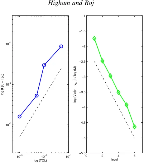
In a separate test, we then fixR=1 and check the convergence behavior. In the left picture of Figure 1 we plot on a log-log scale the accuracy obtained by the multi-level algorithm as a function of TOL for TOL=10−3, 5×10−3, 10−2 and 5×10−2. We see that the algorithm produces an error that scales like TOL. A line with a slope 1 is included for reference.

In the right picture of Figure 1 we plot the quantity log(Var[νl−νl−1])/log(M)over different levels, for a user-specified accuracy of TOL=0.001. A least squares fit for the slope producesq=−0.5525 with a residual of 0.1884. A line with a slope−1

2 is also included for reference. This agrees with the estimate in Higham, Mao, Roj, Song, and Yin (2013), which forms a key part of the complexity analysis.

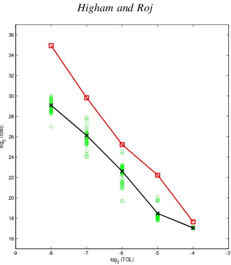
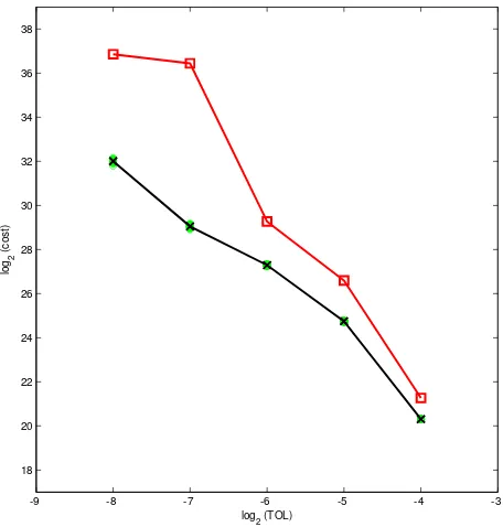
Finally, we compare the computational complexity of standard Monte Carlo with the multi-level version in Figure 2. The computational cost of the multi-level version is measured as

CostMLMC:= N0+

L

∑

l=1 NlMl

!

Table 1: Reference solution was obtained using Monte Carlo simulations,N=5×107,h=10−4. Values in parentheses indicate the half-width of the 95% confidence interval.

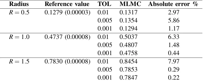
Radius Reference value TOL MLMC Absolute error % R=0.5 0.1279 (0.00003) 0.01 0.1317 2.97

0.005 0.1354 5.86 0.001 0.1294 1.17 R=1.0 0.4737 (0.00008) 0.01 0.5037 6.33 0.005 0.4807 1.48 0.001 0.4758 0.44 R=1.5 0.7830 (0.00008) 0.01 0.8454 7.97 0.005 0.7853 0.29 0.001 0.7847 0.22

whered is the dimension of the approximated process andNl is the number of paths used on each level,

calculated as

Nl=

&

2TOL−2

q

Var[νl−νl−1]M−l

L

∑

l=0

q

Var[νl−νl−1]Ml

!'

, 0≤l≤L. (2)

We measure the computational cost of the standard Monte Carlo method as

CoststdMC:= Nd

h E[τ],

where h is the fixed stepsize such that h=TOL2 and N is the total number of sample paths, chosen adaptively to obtain the required variance. In Figure 2 we plot on a log-log scale the computational cost as a function of the accuracy TOL. For TOL=2−4, 2−5, 2−6, 2−7 and 2−8 we perform 50 multi-level Monte Carlo computations using different initial states of the pseudo-random number generator, and plot the complexity results with green circles. Then we take averages for each accuracy, indicated as black crosses, and compare them with the complexity of standard Monte Carlo, indicated as red squares. A least squares fit performed on the Monte Carlo slope producesq=−4.2156 with a residual 1.0966, and on the multi-level Monte Carlo slope gives q=−3.1688 with a residual of 1.2891. This is in agreement with the analytical results quoted in Section 1: the standard Monte Carlo complexity of O(TOL−4) and the multi-level Monte Carlo complexity ofO(TOL−3|log(TOL)|1/2_).

3.2 Simple Neural Network

We now apply the multi-level Monte Carlo algorithm in a neural network setting. Various models have been considered for the firing of single neurons, but there is an agreement among researchers that if the electrical state of the neural membrane is stated as a single number, which moves towards or away from the firing potential depending on whether the neuron receives excitatory or inhibitory input, respectively, then the time to firing can be estimated by the first hitting time of a certain level for a Brownian motion with drift (Fienberg 1974; Gerstein and Mandelbrot 1964; Iyengar 1985).

Here we are interested in the mean first hitting time of 2-dimensional correlated Brownian motion with driftb,

dXi(s) =bids+σidWi(s),

with constant driftb1=0.1,b2=0.2, constant diffusion coefficientσi=1,i=1,2, initial valueXi(0) =1,

i=1,2 and correlation coefficientρ=−0.5, producing the variance-covariance matrixΣ=

1 −0.5

−0.5 1

10−3 10−2 10−1 10−3

10−2 10−1

log (TOL)

log (E[

τ

] − E[

ν

])

0 2 4 6

−5.5 −5 −4.5 −4 −3.5 −3 −2.5 −2 −1.5 −1

level

log (Var[

νl

−

νl−1

]) / log (M)

Figure 1: Two-dimensional Brownian motion. Left: weak error of the multi-level algorithm. Right: variance ofνl−νl−1 over a sequence of levels.

The Cholesky decomposition ofΣgivesC=

1 −0.5 0 0.8660

, which is then used to simulate correlated Brownian

motions. Fori=1,2 we define the stopping times

τi=inf{t>0 :Xi(t)≤Bi},

where we setB₁=0.5 andB₂=0.25. The quantity of interest is thenE[(τ1∧τ2)∧T]. In Figure 3 we check the convergence rates of the algorithm and variance. The results are consistent with those in subsection 3.1. A least squares fit for the variance slope givesq=−0.5025 with a residual 0.0559.

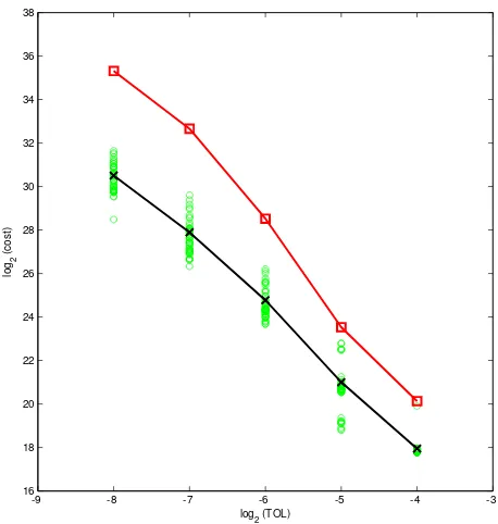
We also check the computational cost of the algorithm in Figure 4. A least squares fit for the standard Monte Carlo slope produces q=−3.9492 with a residual 1.1694, whereas the multi-level method gives q=−3.2004 with a residual 0.5913, confirming the theoretical complexity outlined in Section 1.

3.3 First-to-Default Swaps

Finally, we apply the multi-level Monte Carlo algorithm in a financial setting to basket default swaps used in risk management. These financial instruments are derivative securities tied to an underlying basket of corporate bonds or other assets subject to credit risk. A basket default swap gives the protection buyer a type of insurance against the possibility of default in exchange for regular payments made to the protection seller (Chen and Glasserman 2008). These instruments are popular mainly because insuring a basket of assets is usually cheaper than insuring each asset separately. We focus on the example of a first-to-default swap in which the protection buyer is compensated if any asset in the basket defaults, at which time the contract expires (Joro, Niu, and Na 2004).

-9 -8 -7 -6 -5 -4 -3 16

18 20 22 24 26 28 30 32 34 36

log

2 (TOL)

lo

g2

(

c

o

s

t)

Figure 2: Two-dimensional Brownian motion. Computational cost of standard Monte Carlo (red squares) and multi-level Monte Carlo (green circles). Black crosses indicate averages of multi-level Monte Carlo cost for each accuracy.

2000). Hence, we simulate the underlying processes using a geometric Brownian motion model

dXi(s) =biXi(s)ds+σiXi(s)dWi(s),

with constant drift coefficientb₁=0.11,b₂=0.09,b₃=0.07,b₄=0.04,b₅=0.02, and constant volatility

σ1=0.4,σ2=0.6,σ3=0.8,σ4=0.8,σ5=1. The initial value of each company is set to 1, i.e.,Xi(0) =1,

i=1, . . . ,5. The lower boundary, which is a default level, is set toB=0.1. We are interested in estimating the quantityE[(τ1∧τ2∧τ3∧τ4∧τ5)∧T]. We used Monte Carlo simulations with a fixed timesteph=10−3 andN=5×106 samples to obtain a reference value ofE[τ∧T] =1.2359 for the mean first default time

of the basket. The half-interval width of the 95% confidence interval is 0.0005, making the statistical error negligible.

We use the same format as in the previous two examples. In the right hand picture of Figure 5 a least squares fit for the slope producesq=−0.6049 with a residual of 0.5252.

10−3 ₁₀−2 ₁₀−1

10−3 10−2 10−1

log (TOL)

log (E[

τ

] − E[

ν

])

0 2 4 6 −5.5

−5 −4.5 −4 −3.5 −3 −2.5 −2 −1.5 −1

level

log (Var[

νl

−

νl−1

]) / log (M)

Figure 3: Neural network. Left: weak error of the multi-level algorithm. Right: variance ofνl−νl−1over a sequence of levels.

-9 -8 -7 -6 -5 -4 -3

16 18 20 22 24 26 28 30 32 34 36 38

log

2 (TOL)

lo

g2

(

c

o

s

t)

10−3 ₁₀−2 ₁₀−1

10−3

10−2

10−1

log (TOL)

log (E[

τ

] − E[

ν

])

0 2 4 6

−4.5 −4 −3.5 −3 −2.5 −2 −1.5 −1 −0.5 0

level

log (Var[

νl

−

νl−1

]) / log (M)

Figure 5: First-to-default. Left: weak error of the multi-level algorithm. Right: variance ofνl−νl−1over a sequence of levels.

-9 -8 -7 -6 -5 -4 -3

18 20 22 24 26 28 30 32 34 36 38

log

2 (TOL)

lo

g2

(

c

o

s

t)

ACKNOWLEDGMENTS

MR was supported by the Engineering and Physical Sciences Research Council of the UK, and by Numerical Algorithms Group Ltd. DJH was supported by a Leverhulme Fellowship.

REFERENCES

Andersen, L. 2000. “A Simple Approach to the Pricing of Bermudan Swaptions in the Multi-Factor Libor Market Model”. Journal of Computational Finance3:5–32.

Black, F., and J. Cox. 1976. “Valuing Corporate Securities: Some Effects of Bond Indenture Provisions”. The Journal of Finance 31 (2): 351–367.

Boyle, P., M. Broadie, and P. Glasserman. 1997. “Monte Carlo Methods for Security Pricing”.Journal of Economic Dynamics and Control 21 (8-9): 1267–1321.

Chen, Z., and P. Glasserman. 2008. “Fast Pricing of Basket Default Swaps”.Operations Research56 (2): 286–303.

Crouhy, M., D. Galai, and R. Mark. 2000. “A Comparative Analysis of Current Credit Risk Models”. Journal of Banking & Finance 24 (1-2): 59–117.

Fienberg, S. 1974. “Stochastic Models for Single Neuron Firing Trains: a Survey”. Biometrics 30 (3): 399–427.

Gerstein, G., and B. Mandelbrot. 1964. “Random Walk Models for the Spike Activity of a Single Neuron”. Biophysical Journal4 (1): 41–68.

Giles, M. 2008. “Multilevel Monte Carlo Path Simulation”.Operations Research56 (3): 607–617. Glasserman, P. 2004.Monte Carlo Methods in Financial Engineering. Springer Verlag.

Gobet, E., and S. Menozzi. 2004. “Exact Approximation Rate of Killed Hypoelliptic Diffusions Using the Discrete Euler Scheme”.Stochastic Processes and their Applications112 (2): 201–223.

Gobet, E., and S. Menozzi. 2007. “Discrete Sampling of Functionals of Itˆo Processes”. S´eminaire de Probabilit´es XLXL:355–374.

Gobet, E., and S. Menozzi. 2010. “Stopped Diffusion Processes: Boundary Corrections and Overshoot”. Stochastic Processes and their Applications120 (2): 130–162.

Heinrich, S. 2001. “Multilevel Monte Carlo Methods”. InLecture Notes in Large Scale Scientific Computing, edited by S. Margenov, J. Wasniewski, and P. Yalamov, 58–67: Springer-Verlag.

Higham, D., X. Mao, M. Roj, Q. Song, and G. Yin. 2013. “Mean Exit Times and the Multi-level Monte Carlo Method”.SIAM Journal on Uncertainty Quantificationto appear.

Iyengar, S. 1985. “Hitting Lines with Two-dimensional Brownian Motion”. SIAM Journal on Applied Mathematics45:983–989.

Joro, T., A. Niu, and P. Na. 2004, December. “A Simulation-Based First-to-Default (FtD) Credit Default Swap (CDS) Pricing Approach under Jump-Diffusion”. InProceedings of the 2004 Winter Simulation Conference, edited by R. G. Ingalls, M. D. Rossetti, J. S. Smith, and B. A. Peters, Volume 2, 1632–1636. Piscataway, New Jersey: Institute of Electrical and Electronics Engineers, Inc.

Longstaff, F., and E. Schwartz. 2001. “Valuing American Options by Simulation: A Simple Least-squares Approach”.Review of Financial Studies 14 (1): 113.

Mannella, R. 1999. “Absorbing Boundaries and Optimal Stopping in a Stochastic Differential Equation”. Physics Letters A254 (5): 257–262.

AUTHOR BIOGRAPHIES

Numerical Analysis and Journal of Computational Finance. His research interests lie broadly in numerical analysis, stochastic computation and complexity science. His email address isd.j.higham@strath.ac.ukand his web page ishttp://personal.strath.ac.uk/d.j.higham.