A load sharing system reliability model with managed component degradation

A Load Sharing System Reliability Model with Managed Component

Degradation

Zhisheng Ye,

Member, IEEE

, Matthew Revie, Lesley Walls

Motivated by an industrial problem affecting a water utility, we develop a model for a load sharing system where an operator dispatches work load to components in a manner that manages their degradation. We assume degradation is the dominant failure type, and that the system will not be subject to sudden failure due to a shock. By deriving the time to degradation failure of the system, estimates of system probability of failure are generated, and optimal designs can be obtained to minimize the long run average cost of a future system. The model can be used to support asset maintenance and design decisions. Our model is developed under a common set of core assumptions. That is, the operator allocates work to balance the level of the degradation condition of all components to achieve system performance. A system is assumed to be replaced when the cumulative work load reaches some random threshold. We adopt cumulative work load as the measure of total usage because it represents the primary cause of component degradation. We model the cumulative work load of the system as a monotone increasing and stationary stochastic process. The cumulative work load to degradation failure of a component is assumed to be inverse Gaussian distributed. An example, informed by an industry problem, is presented to illustrate the application of the model under different operating scenarios.

Index Terms—Load sharing system, managed degradation, degradation failure, cumulative work load, gamma process.

ABBREVIATIONS& ACRONYMS

CWL Cumulative Work Load IG Inverse Gaussian RGF Rapid Gravity Filter

NOTATION

T Time to degradation failure of the system

Xi CWL-to-degradation failure of componenti

S CWL-to-degradation failure of the system

U(t) CWL to the system at t

n Number of components in a system

C(τ) Expected cost over mission timeτ Cave Long run average cost

µ Mean of the IG distribution forXi

λ Shape parameter of the IG distribution for Xi

v Rate of accumulation of the CWL process

CO Operational cost of a system

Cr Replacement cost of a system

Cs Fixed system replacement cost

Zhisheng Ye is with the Department of Industrial & Systems Engineering, National University of Singapore, Singapore

I. INTRODUCTION

Our model is motivated by an industrial problem faced by a water utility which sought to make strategic decisions about asset management across their network. We begin by outlining our particular problem before generalising our system context and requirements to set the scene for modeling, and for providing a context for articulating our objectives.

A. Motivating industry problem

A key asset in a water treatment works is a Rapid Gravity Filter (RGF), which is used during the water filtration process. Raw water is input to the filter (e.g., filter sand and gravel), and gravity is used to drain the water through the media to remove impurities so that clean water can be output. With use, the RGF media degrades gradually, and this degradation can be observed through symptoms such as, for example, clustering of the sand within the media leading to a loss of effectiveness in cleaning the water, and residual impurities remaining in the output water leading to reduced purity of the filtered water. The RGF media is believed to degrade with use, and the rate of that degradation might depend on factors, such as the media supplier quality. Degradation of the RGF is observable by the operator through direct inspection of the media, and indirectly through measurements of output water quality. Degradation of the media eventually leads to a failure of the RGF when the overall performance of the media is deemed unsatisfactory by the operator. This condition tends to occur when the quality of the water exiting the RGF does not meet specified targets.

Typically, there are multiple RGFs configured in parallel in a water filtering system, and these RGFs can be activated to simultaneously filter the incoming water. The capability of the installed water filtering system at any water treatment site is designed to meet maximum peak demand. All RGFs may not be required to operate during non-peak periods, and so some may be in cold standby. The decision of how many and which RGFs to operate is made by the human operator. While the goal is to ensure that the clean water output meets required performance quality standards, conversations with operators indicates that they achieve this result by selecting combinations of RGFs which will achieve reliable water filtering system performance. Operators use their knowledge about the degradation condition of the RGFs, and intentionally manage the usage of the RGFs, not just to decide which to operate on any one occasion, but also to inform the remaining life of the RGFs. They do this so that all assets age gracefully at rates that imply balanced levels of degradation of all RGFs at any point in time. This approach ensures that all RGF media fails at approximately the same time.

Minimising the variation in the degradation condition of RGFs implies they should all be available for operation in high load situations because, if some have failed, then the system may not be able to handle a peak load because each RGF has an upper bound on the filtering rate. Because the operator makes decisions to allocate work load that balances the level of the degradation condition of the RGFs in a water filtering system leading to a common end-of-life for a system of RGFS, we have a particular type of load sharing system.

B. Overview of load sharing systems models

Many other industrial examples of load sharing systems exist; each possesses distinctive characteristics depending on the nature of the work load and the manner in which work is shared. For example, electric generators in a power plant, cables in a suspension bridge, pumps in a hydraulic system, the CPUs in a multiprocessor computing system [1], yarn bundles of untwisted cables, and servers in a distributed computer system. Additional examples are given in [2].

For the examples of load sharing systems described in the literature, a common feature is that all components in the system share the work load, and comply with a certain set of load sharing rules until one component suddenly fails, after which the load is automatically re-distributed to the remaining components. A comprehensive discussion about sharing rules (e.g., equal load sharing, tapered load sharing, local load-sharing, etc.) is provided by [3]. The load sharing mechanism introduces dependency between the times to failure among the components, making modeling and inference of such systems different from simpler redundant systems, such as a k-out-of-nsystem [4]. There exists a large literature reporting the analysis of load sharing systems. For example, modeling the reliability of load sharing systems is discussed by, amongst others, [1], [5], [6], [7], while statistical inferences for load sharing models are developed by [8], [9], [10], [11].

C. Rationale of proposed load sharing model

In our context, the work allocation rule means that the components are used intermittently, and so the regular chronological time scale is not applicable for modeling. An alternative is to use the cumulative work load (CWL) processed by each component. We argue that this approach is appropriate because it represents the cumulative usage of a component, which is the root cause of the component degradation. Additionally, the value of the CWL for each component, as well as the system, might be relatively easy to obtain. For example, the total amount of water processed through an RGF might be obtained from a water meter installed at the water outlet of each RGF, while the total amount of water processed by the water treatment site might be read from a meter installed at the water inlet.

The CWL to degradation failure of a component is modeled as a random variable. This random CWL-to-degradation-failure can be regarded as an unknown resource that a component is endowed with at inception. The failure process can be represented by the accumulated usage of a component over time until the cumulative work load reaches the random CWL-to-degradation-failure of the component. Because the system is deemed to fail when its specified performance threshold can no longer be met because the combined degradation of all components has increased to an unsatisfactory level, the CWL-to-degradation-failure of the system is given by the sum of the CWL-to-degradation-failure of all components.

Based on the CWL scale, we propose a novel approach to modeling the reliability of such a load sharing system as described above, and the subsequent cost estimation. More specifically, we treat the CWL process into the system as a stochastic process. Our model captures the operator’s actions to allocate work load to the components with a view to balancing their degradation condition. The system fails when the CWL accumulation process reaches the random CWL-to-degradation-failure of the system, i.e., the sum of the CWL-to-degradation-failure of all components in the system. In addition to the reliability and cost prediction, this approach also enables optimal design of a future system.

The remainder of the paper is organised as follows. In Section II, we describe the model formulation, and articulate our detailed assumptions. Section 3 develops the analysis for the distribution of system CWL-to-degradation-failure, the work load accumulation process, and the distribution of time to degradation failure, examining alternative representations of the work load accumulation process. Cost analysis is presented in Section 4, and includes derivation of the expected cost for a given operational time period, as well as the long term average cost of a given system design. In Section 5, we relax some of our initial assumptions, and so present some extensions of the basic model. An illustrative example is presented in Section 6 using de-sensitised data informed by our water utility problem. Concluding remarks and suggestions for further work are discussed in Section 7.

II. MODELFORMULATION

Consider a load sharing system that consists of n s-identical components as well as an operator. System work load is allocated to the components by the operator. The condition (or performance) of the components degrades with the CWL. The degradation level of components is observable to the operator, and the operator allocates work load to the components to balance their degradation. The degradation of the components ultimately leads to a system failure when the performance of all components is deemed unsatisfactory by the operator because they cross a specified degradation threshold, upon which a system replacement is required.

LetTdenote the time to degradation failure of the system. Given a degradation failure of the system, the CWL-to-degradation-failure of component i, denoted by Xi, is a random variable with a cumulative distribution function (CDF) FX(x), and probability density function (PDF) fX(x). The CWL-to-degradation-failure of the system, denoted by S, is the sum of the CWL-to-degradation-failures of all components.

Based on the above description, the following assumptions are made.

• The CWL to the system is a monotone increasing and stationary stochastic processU(t);t≥0, wheret= 0corresponds to the installation time epoch of the system. That is, fort, s >0, U(t+s)−U(s)iss-independent ofU(s), has positive support, and has the same distribution as U(t).

• During system operation, the operator allocates the work load to the components based on the work load magnitude, and the component degradation levels. Through the choice of components, the degradation levels of all components are managed so that the degradation failures of all components occur at the same time.

• The component CWL-to-degradation-failures Xi, i= 1, . . . , n, are s-independent and identically distributed (i.i.d.), and follow an inverse Gaussian distribution, i.e., Xi ∼ IG(µ, λ), µ, λ≥0, with PDF, and CDF as

fIG(x;µ, λ) =

λ

2πx3

12

exp

−λ(x−µ) 2

2µ2_x

, x >0, (1)

and

FIG(x;µ, λ) = Φ

r

λ x

_x

µ −1

! + exp

_2λ

µ

·Φ −

r

λ x

_x

µ+ 1

!

, x >0, (2)

Remarks:The assumption of an inverse Gaussian distribution for a component with degradation failure is meaningful, because the first passage time of the Wiener process to a fixed threshold conforms to an inverse Gaussian distribution. The IG process was proposed by [16]. It has numerous nice mathematical properties, and it is often used as a subordinator (i.e., random time scale) for the Wiener process in analysis of financial time series data. If the degradation does not follow a Wiener process, the degradation-threshold time to failure can often be described by a Birnbaum-Saunders distribution, which is well approximated by the inverse Gaussian distribution [17]. On the other hand, the cumulative work load over time is always increasing. In addition, the work load is random, but the demand in different time intervals can be regarded as i.i.d. Therefore, a monotone increasing process with stationary increments is appropriate. When there are seasonal effects on the work load accumulation process, the seasonal fluctuation can be taken into account by using a time transformed stochastic process [18].

III. LOADSHARINGSYSTEMFAILUREPROBABILITYDISTRIBUTION

To derive the probability distribution of the system time-to-degradation-failure, we first convolute the distributions of the component CWL-to-degradation-failure to obtain the distribution of the system CWL-to-degradation-failure, then combine this result with the CWL stochastic process to transform back to the chronological time scale.

A. Distribution of system CWL-to-degradation-failure

The moment generating function of the inverse Gaussian variable specified by (1) and (2) is given by

MX(z) =E[exp(zX)] = exp "

λ

µ 1−

r 1−2µ

2_z

λ

!#

. (3)

The CWL-to-degradation-failure of the system is the sum ofXi, i= 1,2, . . . , n, i.e., S= Pn

i=1Xi. The CDF ofSisF

(n)

X (.), the n-fold convolution of FX(.). Generally speaking, the convolution is difficult to obtain. Alternatively, we can consider the moment generating function of S, which is

Ms(z) =E "

exp z

n X

i=1

Xi !#

= exp "

nλ

µ 1−

r 1−2µ

2_z

λ

!#

. (4)

Note that the cumulant on the right hand side can be re-organized as

nλ

µ 1−

r 1−2µ

2_z

λ

! = n

2_λ

nµ 1−

r

1−2(nµ) 2_z

n2_λ

!

.

By comparing (4) with (3), the above equality shows thatS indeed followsIG(nµ, n2_λ).

B. Work load accumulation process

In situations where the incoming work load is relatively steady, the cumulative work load may be approximated by a linear function with rate v. If the approximation holds, the CWL to the system is U(t) = vt. Therefore, the time-to-degradation-failure and the CWL-to-degradation-time-to-degradation-failure satisfies the relationshipvT =S, and thus T =S/v. Using the same technique as presented in Section III-A, we can show that, when S∼ IG(nµ, n2_{λ),T =S/v∼ IG(nµ/v, n}2_λ/v).

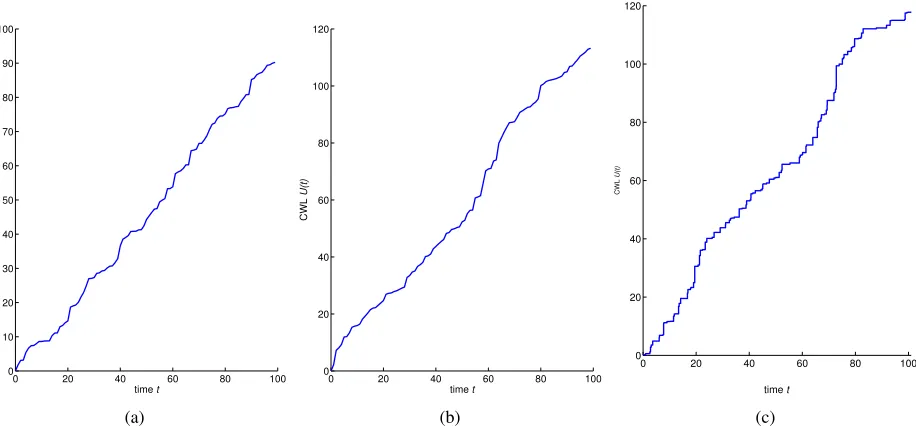
Under an assumption of monotone and stable increments, there exist a number of candidate stochastic processes to describe the CWL over time. As well as the IG process, we shall consider the gamma and compound Poisson processes to describe the work load accumulation. To provide some intuitive insight into the behaviour of these three processes, we illustrate one sample path for each process in Fig. 1. More detailed descriptions of these processes are presented in the following sub-sections.

1) The gamma process

The gamma process, whose sample path is monotone and quite smooth, has been widely used to describe the usage accumulation process of cars or other products, e.g., see [19], and [20], among others. Note that usage is a special case of work load. Therefore, the gamma process is an appropriate candidate for the work load.

The CWL process {U(t);t ≥ 0} is a simple gamma process with stationary increments if it has s-independent, gamma distributed increments. Therefore, U(t)follows Gamma(vt, γ), v, γ >0, with PDF

gU(t)(u;vt, γ) =

γ(γu)vt−1

Γ(vt) exp(−γu), u >0. (5)

The mean, and variance of U(t) are given byvt/γ, andvt/γ2, respectively. If we fix v/γ, and let γ→ ∞, the variance of

0 20 40 60 80 100 0

10 20 30 40 50 60 70 80 90 100

time t

CWL

U

(t

)

(a)

0 20 40 60 80 100

0 20 40 60 80 100 120

time t

CWL

U

(t

)

(b)

0 20 40 60 80 100

0 20 40 60 80 100 120

time t

CWL

U

(t

)

(c)

Fig. 1: The sample path of the Gamma, IG and the compound Poisson processes, all having a mean path function t, and a variance function t: (a) gamma process U(t)∼Gamma(t,1), (b) IG process T ∼ IG(t, t2), (c) compound Poisson process with rate λ(t) = 1and jump sizeWi∼EXP(1)

.

2) The compound Poisson process

The load work may take the form of tasks. For example, a system may be operating only when a task arrives [5], while the resource required to process the task is random. If the task arrival rate is not high, we may need to consider the compound Poisson process for the work load. This need motivates the adoption of a compound Poisson process with

U(t) = N(t)

X

i=1

Wi,

where {N(t);t ≥ 0} is a non-homogeneous Poisson process with rate function λ(t), and Wi are the workloads associated with each arrival, which are i.i.d.

3) The inverse Gaussian process

The IG process has monotone, quite smooth sample paths. It is a limit of the compound Poisson process, with a countably infinite number of jumps in any time interval where each jump size is small [21]. This means that the IG process is suitable to model a process which is an accumulation of many small effects over time, for example, wear, corrosion, damage due to high-frequent yet small shocks, etc. Work load may take the form of tasks or orders, where the tasks arrive as a point process, and each task has a random amount of work load. If the arrival rate is high while the work load in each task is small, e.g., computation tasks to a computer, then the CWL may be well approximated by the IG process. On the other hand, the sample path of an IG process is quite smooth. We expect that the IG process is able to provide a reasonable approximation to some continuous CWL processes. Another attractive property of the IG process is that it is flexible to incorporate random effects. The random effects are useful to describe unobservable factors in the CWL process, such as unknown raw water quality.

An IG process {U(t);t≥0} with stationary increments has s-independent and IG distributed increments, i.e., U(0) = 0, andU(t+s)−U(s)∼ IG(vt, γt2_{)for any s, t >0. The monotone property of the IG process is guaranteed by the positive}

support of the IG distribution. The mean, and variance of U(t)are respectively given by

E[U(t)] =vt, and var[U(t)] =v3t/γ. (6) When we fix v, and let γ → ∞, the variance of this process tends to zero while the mean remains unchanged. This result means that the process degenerates to a deterministic linear accumulation model.

C. Time-to-degradation-failure distribution

To predict the reliability, and estimate the expected costs of the system, it is desirable to know the distribution of the time-to-degradation-failure under the chronological time scale. This knowledge can be achieved by combining the results in Sections 3.1 and 3.2. The time-to-degradation-failure,T, of the system is given by

FT(t) =P r(S < U(t)) = Z ∞

0

Generally speaking, (7) does not bear a closed-form solution. But the integral is only one dimensional, and thus it can be efficiently computed through some numerical techniques. For example, [22] propose an algorithm to compute (7) that is similar to the Riemann sums for the integral except that it partitions unevenly the domain of T to give a greater resolution in high probability density regions.

IV. COSTANALYSIS

Suppose that the unit time operation cost of an n-component system is nCO, depending on the number of components. When the system is replaced because of unsatisfactory performance, the replacement cost includes the price of each component, denoted by Cr, and a fixed system replacement cost, denoted by Cs. The replacement time is assumed negligible compared with the time-to-degradation-failure of the system. This section considers two problems. First, we estimate the expected cost of an existing system operating within a predetermined time horizon. Second, we derive the long term average cost, and the associated optimal system design for a future system.

A. Expected cost of operating system over a finite time horizon

Suppose that a system starts operation at timet= 0. We would like to estimate the expected cost of the system overτunits of time. To compute the expected cost, we treat the replacement process as a renewal process, where the system starts anew after each replacement. The distribution of the inter-replacement time of the renewal process is given byFτ(t)in (7), and the expected cost over time τ is given by

C(τ) =nCOτ+ (nCr+Cs)m(τ).

m(t)is the renewal function of the renewal process. The renewal function generally does not bear a closed form expression, but it can be numerically computed by means of the Riemann-Stieltjes sums algorithm [23]. This algorithm computes the renewal function in a recursive way, and only needs the values ofFT(tj), which are available from (7).

B. Long term average cost, and the optimal design of future system

For an n-component system,T(n)is used to denote the time to system failure. Again we assume that, after each replacement, the system renews. Based on renewal reward processes [24], the long term average cost per unit time can be expressed as

Cave(n) = nCOE[T(n)] +nCr+Cs

E[T(n)] =nCO+

nCr+Cs

E[T(n)] . (8)

Now consider the optimal design of a new system to minimize the long run average cost by properly choosing the number of components n. Usually, there is a lower bound imposed onnbecause of the minimum requirement of the system capacity to deal with peak loads. In addition, there is an upper bound because of the system capacity, e.g., volume or space constraint. Therefore, we consider the optimal design problem as follows.

min

n Cave(n) =nCO+

nCr+Cs

E[T(n)]

s.t.:n≤n≤n¯ (9)

n∈_N

To obtain the optimal solution, we need to simplify the objective function. The following result turns out to be helpful.

Proposition 1. Consider a system with n identical components subject to degradation. Suppose the CWL process has

s-independent and stationary increments while the increment at any time interval has a continuous distribution with support on

(0,∞) . If the usage rule is to keep the degradation of all components at the same level, thenE[T(n)] =nE[T(1)], where

T(1) is the lifetime of a system with a single component.

The proof is given in the Appendix. Given this proposition, the objective function in (9) can be specified as

Cave(n) =nCOE[T(n)] +nCr+Cs

E[T(n)] =nCO+

Cs

nE[T(1)]+

Cr

E[T(1)]. (10)

It is readily seen that (10) is a convex function of n. If we treat n as continuous in (10), the minimum is achieved at

n† =pCs/(COE[T(1)]). In addition,Cave(n)is decreasing whenn < n†, and increasing whenn > n†. Therefore, given the constraints in (9), whenn≥n†,Cave(n)is increasing in the interval[n,¯n], and the minimum of (9) is achieved atn. On the other hand, if n¯≤n†,Cave(n)is decreasing in the interval[n,¯n], and thus¯nminimizes (9). Based on the above discussion, the optimal solution of (9) is recapitulated in the following proposition.

Proposition 2.Suppose the conditions specified in (9) hold. Then the optimal solution of (9) is specified as follows.

• When ¯n≤n†,n∗= ¯n.

• When n < n1<n¯,n∗=bn†cordn†e, whichever yields a lower cost.

See from Proposition 2 that, when all components ares-identical, the optimal system configuration that minimizes the long run average cost is easy to obtain. Even when the components are nots-identical (e.g. they come from a number of suppliers), then the determination of the optimal system design configurations is also not difficult, as we shall discuss further in Section 5.3.

V. EXTENDING THEMODEL TOMULTIPLECOMPONENTCHOICES

In Sections 2 through 4, we have presented a model for a single n-component system, where all components are assumed new ands-identical. We now relax that assumption, and consider the scenario when the system has non-s-identical components. Components in the system need not bes-identical; the same components may be sourced from different suppliers, or a single supplier may provide variants of the same component. Let us now extend the model to represent non-s-identical components, and to frame decisions in terms of the optimal choice of components.

Suppose that there are m suppliers, the price of a component from supplier i is Cr(i), while the unit time operational cost of the component is C_O(i). A system is comprised of ni components from supplier i. Let n= (n1, n2, . . . , nm)0 be the

configuration of the system, and T(n) be the time-to-degradation-failure of this system. It is readily seen that T(ei)is the time-to-degradation-failure of a system with a single component from supplier i, where ei is the unit vector with the i-th element equal to 1 while others are equal to 0. The distribution of T(ei) depends on the CWL process, and the quality of the component. Similar to Section 4, we are concerned with two questions: (a) how to estimate the expected cost over a finite time horizon for an existing system, and (b) how to select the optimal configurationnfor a new system.

A. Cost estimation of operating system over a finite time horizon

Consider a system with configurationn. The total expected cost of the system overτ units of time includes the operational cost, and the replacement cost, which can be specified as

C(τ) =τ

m X

i=1

niC

(i)

O + m X

i=1

niCr(i)+Cs !

m(τ) =τn0CO+ (n0Cr+CS)m(n, τ), (11)

where Cr =

Cr(1), . . . , Cr(m) 0

, CO =

C_O(1), . . . , C_O(m)

0

, and m(n, τ) is the expected number of replacements over τ. To use the Riemann-Stieltjes sums algorithm to numerically evaluate m(n, τ), the distribution ofT(n)is needed, which is discussed below.

For a system with configuration n, its time-to-degradation-failure distribution depends on the CWL process, and the CWL-to-degradation-failure of the system S(n). The CWL process can be adopted directly from Section 3.2, and the CWL-to-degradation-failure of the system is the sum of the CWL-to-degradation-failure of the components, i.e., S(n) = Pm

i=1

Pni

j=1Xi:j, whereXi:j is the CWL-to-degradation-failure of thejth unit from theith supplier, andXi:1, . . . , Xi:ni are

i.i.d. random variables following the same IG distribution. Generally speaking, S(n)is no longer an IG variable. However, it is reasonable to assume thatXi:j∼ IG(ηi, λ0η2i), under which it can be shown thatS(n)∼ IG(η, λ0η2)withη=

Pm i=1niηi by following a similar procedure to that in Section 3.1. Our justification for the form of the IG distribution is as follows.

Recall that the components are subject to failures caused by gradual degradation. Consider that the component degradation follows a Wiener process with W(u) = vu+σvB(u), where v, and σ are respectively the drift, and volatility parameters.

B(u) is the standard Brownian motion, and u is the CWL. We use the Wiener process of this form by considering that a unit with high degradation rate v will also have high variance rate σv. Then the first passage CWL of this process to a fixed thresholdD follows anIG distributionIG D/v, D2_/(σ2_v2₎

. We may assume that the components from different suppliers have different degradation rate v, but the same volatility parameter σ. Then the CWL-to-degradation-failure of a component from supplieriisIG D/vi, D2/(σ2vi2)

, which can be denoted asIG(ηi, λ0η2i)withηi=Di/vi, andλ0=σ−2. The above

reasoning justifies the assumption of the form of IG distribution.

Given the distribution ofS(n), we can follow the same procedure in Section 3.3 to compute the distribution of the system lifetime T(n).

Remark: If there are multiple systems in operation, then different systems may have different CWL processes{U(t);t≥0}, and distinct configurations, i.e., different n. For each system, we can compute the distribution of their time-to-degradation-failure T(n)based on its CWL process and configuration, and then evaluate the expected cost using (10).

B. Optimal design of a future system

Proposition 3. Consider a system with the combination of componentsn= (n1, n2, . . . , nm)0, where ni is the number of

components from supplier i. Given the conditions in Proposition 1, we have E[T(n)] =Pm_i=1niE[T(ei)].

The proof of this proposition is similar to that of Proposition 1, and thus is not presented here. Given this proposition, the long term average cost of the system with n= (n1, n2, . . . , nm)0 and the optimal design problem can be expressed as

min n

¯

Cave(n) = Pm

i=1

Pm

j=1ninjC

(i)

O E[T(ej)] + Pm

i=1niC

(i)

r +Cs Pm

i=1niE[T(ei)]

= n

0_Qn+n0_C

r+Cs

n0_T (12)

s.t.:n≤n01m≤¯n

n∈_N

where T = (E[T(e1)], . . . , E[T(em)])0,1m = (1, . . . ,1), and Q = (COT0+T CO0 )/2 is a symmetric matrix. Equation (12) is a quadratic-linear fractional integer programming problem with linear constraints. If Q is positive semi-definite, then (12) is a convex-concave type nonlinear fractional programming problem, and the objective function is quasi-concave [25]. Therefore, a global maximum can in principle be obtained through a local maximization algorithm. But the matrix Q in our problem is found to be indefinite. In this case, we may invoke the algorithm developed by [26] to solve (12) without the integer constraint, and then search the feasible integer points around the solution. Alternatively, local search algorithms like tabu search or evolutionary methods like genetic algorithm can be used to obtain a local optimal solution when the dimension of nis large. In situations where the number of suppliers is small, then an exhaustive enumeration may be feasible.

VI. ILLUSTRATIVEEXAMPLE

Informed by our motivating industry example, but using de-sensitised data, we present examples of our model under a number of scenarios. We begin with the case of a single system comprising identical components. The analysis is then extended to allow for multiple suppliers of components.

A. Analysis of a single system with identical components

An existing system has 5 components with i.i.d. CWL-to-degradation-failureXi, whereµ= 2000, andλ= 5000. The CWL process {U(t);t≥0} is modeled using a Gamma process such thatU(t)∼Gamma(vt, γ) withv = 1000, andγ = 1. The operational cost for each component is CO = 0.05 per year, the price of a component isCr= 1, and the fixed replacement cost is Cs= 5. The units used for the time, monetary values, and the CWL are in years, millions of pounds, and trillion of litres, respectively.

1) Reliability and cost under different operational experience scenarios

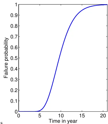
Suppose the system has all new components att= 0. Based on Section 3.1, the CWL-to-degradation-failureS of the system is given by an IG(10000,125000). Therefore, the time to failure distribution (7) of the system can be computed numerically. The resulting CDF of the time-to-degradation-failure distribution, T(5), is depicted by the solid line in Fig. 2. By year 5, the probability of surviving remains close to 1, but by year 10 it has fallen to around 0.4, and by year 20 the system will almost certainly have failed.

Based on the distribution of the system time-to-degradation-failure T(5), the expected number of replacements and the expected cost of the system over time can be obtained based on the results in Section 4.1, as can be seen from the solid lines in Fig. 3. For example, by year 5, there are no expected renewals, and the expected cost over this horizon is around £1.3m. One replacement is expected by year 16, by which time the expected cost is £15.2m.

2) Optimal design of future system

Suppose now that we would like to design a new system, and the objective is to choose the optimalnto minimize the long run average cost subject to the constraint that 4≤n≤10. To use the results in Section 4.2, we need to compute E[T(1)], which we find to be 2.006. Without the integer constraint, the minimal cost is achieved whenn†= 7.06. Based on Proposition 2, we can check the long run average costs whenn= 7, andn= 8, which we find to be£1.205m, and£1.214m, respectively. Therefore, the optimal design should ben∗= 7. The long run average cost over the number of components is shown in Fig. 4, which suggests n∗= 7.

B. Analysis given non-identical components from two suppliers

ss

0 5 10 15 20

0 0.1 0.2 0.3 0.4 0.5 0.6 0.7 0.8 0.9 1

Time in year

Failure probability

Fig. 2: Time-to-degradation-failure distribution for a new system with 5 identical components.

0 5 10 15 20 25

0 0.5 1 1.5 2 2.5

Time in year

Renewal

(a)

0 5 10 15 20 25

0 5 10 15 20 25 30

Time in year

Total cost

(b)

Fig. 3: (a) Expected number of system replacements, and (b) the expected costs over time for a new system of 5 identical components.

follows IG(9200,96800). The work load accumulation process is assumed to be the same for all components regardless of source. The fixed replacement cost is again Cs= 5. For the component from supplier 1, the price of each unit is C

(1)

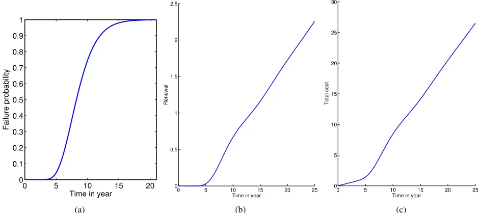
r = 1, and the operational cost is C_O(1) = 0.05 per year. For the component from supplier 2, the price of each unit is Cr(2) = 0.2, and the operational cost isC_O(2)= 0.03per year. As before, the units used for the time, monetary values, and the CWL are in year, millions of pounds, and trillion of litres, respectively.

ss 4 5 6 7 8 9 10

1.2 1.22 1.24 1.26 1.28 1.3 1.32 1.34

Number of components

Ccost

Fig. 4: The long run average cost of the system of 5 identical components as a function of the number of components.

0 5 10 15 20 0

0.1 0.2 0.3 0.4 0.5 0.6 0.7 0.8 0.9 1

Time in year

Failure probability

(a)

0 5 10 15 20 25

0 0.5 1 1.5 2 2.5

Time in year

Renewal

(b)

0 5 10 15 20 25

0 5 10 15 20 25 30

Time in year

Total cost

(c)

Fig. 5: (a) Probability of failure, (b) expected number of replacements, and (c) the expected costs over time for a new system of 5 components with 4 from Supplier 1 and the other from Supplier 2.

put into operation at t= 0.

Given the cost structure, if we would like to design a new system in the future, and assuming that we would continue to source from the two suppliers, then the optimal design that minimizes the long run average cost can be derived based on the results in Section 5.2. The optimal cost is£1.163m, and the associated optimal configuration isn∗= (2,8)0, i.e., 2 components from supplier 1, and 8 components from supplier 2.

VII. CONCLUDINGREMARKS,ANDFUTUREWORK

chronological time scale is used. These aspects of the problem motivate consideration of the CWL as the time scale instead of using chronological time. We have discussed the gamma, inverse Gaussian, and the compound Poisson processes to describe alternative representations of the CWL over time. Because we consider only component failures that are caused by degradation, we model the CWL-to-degradation-failure of the components by the inverse Gaussian random variable. Based on the CWL process, and the CWL-to-degradation-failure distributions, the time-to-degradation-failure of the system can be derived.

In settings where the components in the system are identical, as might be the case if all are of the same type sourced from a single supplier, the CWL-to-degradation-failure of the system is again inverse Gaussian distributed. The expected cost of an existing system, and the optimal design of a future system that minimizes the long run average cost have been derived. There may be situations where all components are not identical, say when there are multiple suppliers of the same component, or variants of the component type available from the same supplier. Under mild assumptions, the CWL-to-degradation-failure of the system can also be modeled by the inverse Gaussian distribution, and the expected cost can be derived in a similar way. The optimal design is a quadratic-linear fractional integer programming problem, but the quadratic part is not positive semi-definite. If the number of suppliers is small, then the optimization can be implemented using existing software packages for integer programming, or even through enumeration.

Our model has been motivated by an industry problem facing a water utility. Our example is informed by this problem although it has been designed to illustrate implementation of our model and interpretation of the analysis only. Here we have specified parameter values that might be deemed reasonable for illustrative purposes. To use the model, we need to develop methods for obtaining data to support parameter estimation and model fitting. We might expect data collection to be a combination of statistical observations and structured expert judgment [27]. Expert judgment can provide subjective assessments of parameter uncertainty. Goodness-of-fit tests using empirical data can support selection of appropriate processes for the CWL process [28], [29], and to verify the IG distribution for the CWL-to-degradation failure of the components.

As well as developing statistical inference methods for our model, there are a number of ways in which it might be extended. To date, we have focused attention on a single system; however, multiple systems may exist. For example, our water utility operates over 70 water treatment sites which are geographically located over diverse environments with variations in the quality of the raw water. Therefore, it would be beneficial to introduce random-effects into the CWL process, with the random-effects representing the unobservable raw water quality. Moreover, a system may have been in operation for a number of years rather than starting operation at t= 0. Cost analysis of such a system should be considered. It would also be useful to relax some assumptions because we made quite strong assumptions about how closely the operator can observe the component degradation, and therefore how well degradation can be controlled. However, there may be occasions due to, for example, seasonal characteristics where it is not possible to shut down certain RGFs because all are required to meet demand, and so degradation is not managed as we have assumed. Therefore, further work may also involve thinking about which factors affect the manner in which the system is being used when the cumulative work load is high, and system performance is close to its critical threshold.

APPENDIX

Consider a system with n identical components, each with CWL-to-degradation-failure Xi, i = 1,· · · , n. The time-to-degradation-failure of the system Tn is defined as the event that U(t) hits

Pn

i=1Xi. In fact, this failure process can be separated intonsteps: at the first step,U(t)reachesX1at timeZ1. Because the increment at any time interval has a continuous

distribution with support on (0,∞), we can know thatU(Z1) =X1. The second step begins at time Z1 withU(Z1) =X1,

and ends at Z2 withU(Z2) =X1+X2. Similarly, the kth step, 2≤k≤n, starts at Zk−1 withU(Zk−1) =Pkj=1−1Xj, and ends at Zk with U(Zk) = Pk_j=1Xj. Obviously, Tn = Zn. Given that the usage process has s-independent and stationary increments, Z1, Z2−Z1,· · · , Zn−Zn−1 haves-independent and identical distributions. Therefore,

E[Tn] =E[Zn] =E "

Z1+

n X

k=2

Zk−Zk−1

#

=nE[Z1]. (13)

By observing that Z1 is equivalent to the time-to-degradation-failure of a single component system under the same usage

process, the proposition follows.

ACKNOWLEDGEMENTS

We would like to thank Scottish Water and the UK Technology Strategy Board for funding the Knowledge Transfer Partnership between the Universities of Strathclyde and Edinburgh with Scottish Water, which provided the problem motivation. We would especially like to thank the Analytics team at Scottish Water for discussions about the motivating problem.

REFERENCES

[1] H. Liu, “Reliability of a load-sharing k-out-of-n: G system: non-iid components with arbitrary distributions,”IEEE Transactions on Reliability, vol. 47, no. 3, pp. 279–284, 1998.

[2] P. H. Kvam and E. A. Pena, “Estimating load-sharing properties in a dynamic reliability system,”Journal of the American Statistical Association, vol. 100, no. 469, pp. 262–272, 2005.

[3] S. Durham, J. Lynch, W. Padgett, T. Horan, W. Owen, and J. Surles, “Localized load-sharing rules and markov-weibull fibers: a comparison of microcomposite failure data with monte carlo simulations,”Journal of composite materials, vol. 31, no. 18, pp. 1856–1882, 1997.

[4] W. Kuo and M. J. Zuo,Optimal Reliability Modeling: Principles and Applications. Hoboken: John Wiley & Sons, 2003.

[5] L. Huang and Q. Xu, “Lifetime reliability for load-sharing redundant systems with arbitrary failure distributions,”IEEE Transactions on Reliability, vol. 59, no. 2, pp. 319–330, 2010.

[6] M. Finkelstein, “On systems with shared resources and optimal switching strategies,” Reliability Engineering & System Safety, vol. 94, no. 8, pp. 1358–1362, 2009.

[7] ——,Failure rate modelling for reliability and risk. Springer, 2008.

[8] H. Kim and P. Kvam, “Reliability estimation based on system data with an unknown load share rule,”Lifetime Data Analysis, vol. 10, no. 1, pp. 83–94, 2004.

[9] C. Park, “Parameter estimation for the reliability of load-sharing systems,”IIE Transactions, vol. 42, no. 10, pp. 753–765, 2010.

[10] ——, “Parameter estimation from load-sharing system data using the expectationmaximization algorithm,”IIE Transactions, vol. 45, no. 2, pp. 147–163, 2013.

[11] B. Singh, K. K. Sharma, and A. Kumar, “A classical and bayesian estimation of a k-components load-sharing parallel system,”Computational Statistics & Data Analysis, vol. 52, no. 12, pp. 5175–5185, 2008.

[12] C. Park and W. J. Padgett, “Accelerated degradation models for failure based on geometric brownian motion and gamma processes,”Lifetime Data Analysis, vol. 11, no. 4, pp. 511–527, 2005.

[13] ——, “Stochastic degradation models with several accelerating variables,”IEEE Transactions on Reliability, vol. 55, no. 2, pp. 379–390, 2006. [14] Z. S. Ye, M. Xie, L. C. Tang, and Y. Shen, “Degradation-based burn-in planning under competing risks,”Technometrics, vol. 54, no. 2, pp. 159–168,

2012.

[15] IEV-191-04-22, “Degradation failure,” 2012.

[16] M. T. Wasan, “On an inverse gaussian process,”Skandinavisk Aktuarietidskrift, vol. 51, pp. 69–96, 1968.

[17] A. Desmond, “On the relationship between two fatigue-life models,”IEEE Transactions on Reliability, vol. 35, no. 2, pp. 167–169, 1986.

[18] G. A. Whitmore and F. Schenkelberg, “Modelling accelerated degradation data using wiener diffusion with a time scale transformation,”Lifetime Data Analysis, vol. 3, no. 1, pp. 27–45, 1997.

[19] N. D. Singpurwalla and S. Wilson, “Failure models indexed by two scales,”Advances in Applied Probability, vol. 30, no. 4, pp. 1058–1072, 1998. [20] J. F. Lawless and M. J. Crowder, “Models and estimation for systems with recurrent events and usage processes,”Lifetime Data Analysis, vol. 16, no. 4,

pp. 1–24, 2010.

[21] Z. S. Ye and N. Chen, “The inverse gaussian process as a degradation model,”Technometrics, p. to appear, 2013.

[22] Z. S. Ye, Y. Shen, and M. Xie, “Degradation-based burn-in with preventive maintenance,”European Journal of Operational Research, vol. 221, no. 2, pp. 360–367, 2012.

[23] M. Xie, “On the solution of renewal-type integral equations,”Communications in Statistics-Simulation and Computation, vol. 18, no. 1, pp. 281–293, 1989.

[24] S. M. Ross,Introduction to Probability Models, 9th ed. Academic Press, 2007.

[25] W. Dinkelbach, “On nonlinear fractional programming,”Management Science, pp. 492–498, 1967.

[26] A. Beck, A. Ben-Tal, and M. Teboulle, “Finding a global optimal solution for a quadratically constrained fractional quadratic problem with applications to the regularized total least squares,”SIAM Journal on Matrix Analysis and Applications, vol. 28, no. 2, p. 425, 2006.

[27] T. Bedford, J. Quigley, and L. Walls, “Expert elicitation for reliable system design,”Statistical Science, pp. 428–450, 2006.

[28] V. Bagdonavicius and M. S. Nikulin, “Estimation in degradation models with explanatory variables,”Lifetime Data Analysis, vol. 7, no. 1, pp. 85–103, 2000.

[29] J. F. Lawless and M. J. Crowder, “Covariates and random effects in a gamma process model with application to degradation and failure,”Lifetime Data Analysis, vol. 10, no. 3, pp. 213–227, 2004.

Zhi-Sheng Ye (M’13) received a joint B.E. (2008) in Material Science & Engineering, and Economics from Tsinghua University. He received a Ph.D. degree from National University of Singapore. He is currently an Assistant Professor at the Department of Industrial & Systems Engineering, National University of Singapore. His work has appeared in various peer reviewed journals, including Annals Applied Stat., Annals of Oper. Res., Euro. J. Oper. Res., IEEE Trans. Reliab., IIE Trans., J. Applied Stat., J. Qual. Tech., Reliab. Eng. Syst. Safety, and Technometrics. His research areas include industrial statistics, degradation analysis, and reliability modeling.

Matthew Revie received the BSc degree in Pure Mathematics from Glasgow University, Glasgow, UK; and a MSc degree in Operational Research, and the PhD in Management Science, both from the University of Strathclyde, UK. Matthew Revie is currently with the Department of Management Science at the University of Strathclyde, Glasgow, UK. His research interests include modelling reliability and maintainability, degradation, and risk management. Matthew has published in many international journals including Reliab. Eng. Syst. Safety, Risk Analysis, and IEEE Trans. on Eng. Manag. In 2010, along with Tim Bedford and Lesley Walls, he was awarded the 2010 SAGE Best Paper Award by the Journal of Risk and Reliability.