A Gamma kL Transition Model for Transitional Flow with Pressure Gradient Effects

Article

A





k

_L

Transition Model for Transitional Flow with

Pressure Gradient Effects

Ekachai Juntasaro

a,

_*

_{and Abdul Ahad Narejo}

b

Department of Mechanical and Process Engineering, the Sirindhorn International Thai-German Graduate School of Engineering (TGGS), King Mongkut’s University of Technology North Bangkok, Bangkok 10800, Thailand.

E-mail: a_{[email protected] (Corresponding author),} b_{[email protected]}

Abstract. A new and complete version of the



kL transition model has been

continually developed and proposed in the present paper. This version of the



kL

transition model can predict the effects of pressure gradient on the mean flow. The



k_L transition model is validated with the ERCOFTAC T3- and T3C-series

experimental data of Coupland [1]. The validation shows that the computed results of the



k_L transition model are in good agreement with the experimental data. The

performance of the



kL transition model is assessed in comparison with those of the

L

k transition model of Walters and Cokljat [2], the



Re transition model of Langtry

and Menter [3], and the



transition model of Ge et al [4] in case of the transitional flow through the compressor blade passage of Zaki et al [5]. It is found that the proposed



k_L transition model is the only transition model that can consistently capture the separation bubble on the compressor blade.

Keywords: RANS, transition model, intermittency, laminar kinetic energy, pressure gradient.

ENGINEERING JOURNAL Volume 21 Issue 2

1.

Introduction

Transition from laminar to turbulent flow is significant in modern and future engineering applications. Only a few examples are given here. The first example is gas turbine engines where the effect of transitional flow on the design of gas turbine engines was critically studied by Mayle [6]. Another example is the design of wind turbines in which case transition modelling is essentially needed because the prediction could be significantly improved by the transition model compared to the turbulence model as demonstrated in Menter et al [7]. A hypersonic future aircraft is one of the challenging examples where transition modelling plays a key role to the success of hypersonic propulsion system simulation, as mentioned in Georgiadis et al [8], because the laminar flow takes place over a large proportion of the aircraft forebody which is employed as part of the scramjet engine inlet. The state of the inflow into the scramjet engine and the thermal load on the aircraft forebody are greatly affected by the flow transition.

The first ever study on transition perhaps started when Emmons [9] proposed a theory by using a probability function to quantitatively formulate the transition process from laminar to turbulent flow on a flat plate in which the local skin friction coefficient was considered. To the best of the authors’ knowledge, the probability function that was used by Emmons [9] to define the fraction of the total time that the flow is turbulent at any point in the transition region was named for the first time as an intermittency factor



by Schubauer and Klebanoff [10]. Dhawan and Narasimha [11] reported a single universal distribution of the intermittency factor



that was found to be defined as a function of the normalized streamwise coordinate in the transition region of the boundary layer on a flat plate. Furthermore, Dhawan and Narasimha [11] proposed a simple mathematical model to predict the mean flow in the transition zone by using a linear combination of the laminar flow and the turbulent flow with the proportions of (1) and



_{respectively:}     



1  



_L  _T where the overbar denotes the mean flow, the subscript L denotes the laminar flow, and the subscript T _{denotes the turbulent flow. Since then, there have been various ways}

that were proposed for transition modelling in the literature.

Dick and Elsner [12] as editors collected a set of 18 papers for an overview of the knowledge on most important aspects of transition physics and on developed modelling methods. Recently, Fu and Wang [13] provided a comprehensive review on RANS modelling of flow transition in which the review of low-Reynolds-number turbulence models that were applied to transition predictions was given. Therefore, only transition models will be reviewed here in more detail. The development of transition models can be categorized into 2 main directions: one based on the transport equation of the intermittency factor



and the other based on the transport equation of the laminar kinetic energy kL.

The development of the transport equation for the intermittency factor



_{started around 1975 when} Libby [14] and Dopazo [15] attempted to construct the transport equation for



_{using the conditioned} averages to describe the interface dynamics for the interaction between the turbulent part and the non-turbulent part at the outer-edge intermittent region of non-turbulent shear flows. Vancoillie and Dick [16] and Steelant and Dick [17] adopted such a conditioned-average concept to construct the conditionally averaged Navier-Stokes equations in conjunction with the intermittency factor



to predict the transitional flow. In Vancoillie and Dick [16], the intermittency factor



was algebraically prescribed according to Dhawan and Narasimha [11]. The transport equation of



was derived by Steelant and Dick [17] based on (starting

from) the algebraic description of



in the streamwise direction proposed by Dhawan and Narasimha [11].

To be compatible with the conventional RANS modelling framework, Suzen and Huang [19] proposed the transport equation for the intermittency factor



based on a combination of the source terms adopted from Steelant and Dick [17] and Cho and Chung [20] in order to reproduce the streamwise and cross-stream variations of the intermittency factor



in the transition zone. The transitional effect on the mean flow was taken into account by multiplying the eddy viscosity



T by the intermittency factor



in the

diffusion terms of the Reynolds-averaged momentum equations. To account for the turbulent effect on the

mean flow via the eddy viscosity



T, the SST k



turbulence model of Menter [21] was employed as a

baseline turbulence model.

Menter, Esch and Kubacki [22] proposed the transport equation for the generalized intermittency variable based on experimental correlations in which case the momentum-thickness Reynolds number was

linked to the vorticity Reynolds number 

 

 y2

Re _{by adopting the concept of van Driest and Blumer [23]}

so that only local variables were employed and hence the integral or non-local parameters, i.e. the momentum thickness



or free-stream turbulence intensity Tu, could be avoided. Their transition model

interacted with the SST k



turbulence model via the production term of the k equation only. Continually, Menter et al [24] proposed a general framework for the correlation-based



Re transition

model in which the transport equations for the intermittency factor



and the transition momentum-thickness Reynolds number Re were constructed so that their transition model could be implemented _t into the general-purpose unstructured and parallelized CFD code. Their transition model interacted with the SST k



_{turbulence model via both the production and destruction terms of the} kequation. However, two correlations were not provided at that time: Rec to control the location of transition onset

and Flength to control the length of transition region. The complete version of the correlation-based



Re

transition model with the given correlations for Rec and Flength was published later by Langtry and Menter

in [3].

Durbin [25] proposed an empirical transport equation for the intermittency factor, based on local variables without experimental correlations, in which the diffusion of free-stream turbulence (disturbances) into the boundary layer was used to initiate the transition and the source term was employed to control the transition process. The intermittency factor obtained was then used to alter the production term of the k

equation only. The k



_{turbulence model with a set of constants from Wilcox [26] was adopted. Ge,}

Arolla and Durbin [4] further improved the



equation of Durbin [25] by adding a sink term in order to

preserve the laminar region before transition and this sink term disappeared in the turbulent region. Once the intermittency factor was obtained, it was further modified in order to account for the separation-induced transition. Duraisamy and Durbin [27] reported the potential of using the data-driven approach for transition modelling in which the modelling information was extracted from data using inverse solutions and then such information was converted into modelling knowledge using machine learning techniques.

The concept of the laminar kinetic energy k_L started in 1997 when Mayle and Schulz [28] proposed the transport equation for the laminar kinetic energy to predict the streamwise fluctuations in the laminar boundary layer underneath free-stream turbulence before the onset of transition (the pre-transitional flow), and eventually to predict the onset of transition.

Walters and Leylek [29] extended the laminar kinetic energy concept of Mayle and Schulz [28] by constructing the transport equation for the laminar kinetic energy kL in conjunction with the modified





k turbulence model in which the energy of the streamwise fluctuations in the pre-transition zone is transferred to the turbulent kinetic energy via the redistribution mechanisms. Walters and Leylek [30] improved their 2004 version by incorporating the transport equation of the laminar kinetic energy kL with

the modified k



turbulence model in order to better predict the transition breakdown process when the

adverse pressure gradients were present. Walters and Cokljat [2] continually improved the 2005 version to provide a useful and practical tool over a wide range of complex flow conditions.

Menter, [3]). The



Re _{transition model is correlation-based so that it is viable only within a range of}

flow conditions that the experiments were set up to obtain such correlations. The kLtransition model is

physics-based so that itcan be applied over a wider range of flow conditions. However, the modeling scheme of the k_L transition model is insufficient and one more transport equation for



is required to complete the relationship among



, k _and k_L , according to the definition of



, as mentioned in

Juntasaro and Ngiamsoongnirn [31]. Therefore, Juntasaro and Ngiamsoongnirn [31] proposed a new



kL

transition model in whichthe



 equation was derived from the definition of



using the existing transport equations of k and k_{L. However, their}



k_L transition model was validated only for the case of the transitional boundary layer on a flat plate without pressure gradient at various free-stream turbulence levels. Moreover, during the development of their



kL transition model, two non-linear terms, i.e.

 



 

 

  

  _{ } _  _ T_{k }x_{j }

2 2

1 and

 

 

   

_  _{  } 

 

T L

L k j j

k

k x x

2

, in the intermittency transport equation were

omitted due to the numerical difficulty of the singularity existence when the flow becomes fully turbulent in which case the intermittency factor is equal to unity and the laminar kinetic energy is equal to zero. For

compensation, Juntasaro and Ngiamsoongnirn [31] used the extra term 







 



 

 _{  }

 _{ }

 

T

k j

k

k x

2

2 1

to

balance the transition mechanism in the intermittency transport equation. Therefore, the present research work is aimed to propose a new and complete version of the



kL transition model that satisfies the

following objectives:

(a) the new



kL transition model can handle the singularity problem in the fully turbulent flow

regime after including those two non-linear terms into the intermittency transport equation of the



k_L transition model and excluding the extra term 







 



 

 _{  }

 _{ }

 

T

k j

k

k x

2

2 1

that was previously

used for compensation in Juntasaro and Ngiamsoongnirn [31];

(b) the new



kL transition model can take into account the effect of pressure gradient;

(c) the performance of the new



kL transition model is to be assessed in a complex-flow problem.

2.

Model Development

The derivation of the transport equation for



will be described in Subsection 2.1. How to take into account the effect of pressure gradient in the



kL transition model will be expressed in Subsection 2.2.

Subsection 2.3 will provide a summary of the



kL transition model for transitional flow with pressure

gradient.

2.1. Derivation of a Transport Equation for



Following Juntasaro and Ngiamsoongnirn [31], the definition of an intermittency factor



for modelling purpose is given as

   _L

k

k k (1)

where k is the turbulent kinetic energy and kL is the laminar kinetic energy. In order to derive the

 

 

_{ }



1  L

k k (2)

Now, the transport equations of k and kL are needed for use in derivation which are given

respectively as follows:

               

 j   _ T _ _ k

j j k j

k _U k k _S

t x x x (3)



 

   

   

   _  _ L

L L L

j k

j j j

k _U k k _S

t x x x (4)

where Eq. (3) is the kequation from the SST k



turbulence model of Menter [21], Eq. (4) is the kL 

equation from the kL transition model of Walters and Cokljat [2], Sk denotes the source/sink terms of the



k equation, and Sk_L denotes the source/sink terms of the kL equation. After substituting Eq. (2) into

Eq. (3), the resulting equation is

















                         _{ }  _{ }              _ _ _ _           _   _  _ _   _                  _  _  _  _{ }      _{ }  _{   } 2 2 2 3 1 1 + 1 1 2 2 + + 1 1

L L L

j j

j j

L T T L

j k j j k j

T L L T

k j j k j

k k k

U U

t x t x

k k

x x x x

k k

x x x 

2

+S_k

(5)

After multiplying Eq. (5) by 



 1

and then using Eq. (4) for subtraction, the resulting equation is

















    _                                              _  _   _{ } _  _  _                 _{ } _    _{ }    _{  } _ 2 2 + 1 1 2 2 1

+ + + S

1 1 L

L L T T L

j

j j k j j k j

T L L T

k k

k j j k j

k k k

U

t x x x x x

k k

S

x x x

(6)

After multiplying Eq. (6) by 



1



L

k and thenre-arranging with the aid of







2 



₁



1

L

k k

, the

resulting equation is













      _                         _  _  _  _  _         _{ } _  _  _              _ _{ }   _{ }_ _          2 1 + 1 1 2 2

+ + + S

1 L

T T L

j

j j k j L j k j

T L T

k k

L k j j k j L

k U

t x x x k x x

k

S

k x x x k k

(7)









        _                        _  _  _  _{  }  _{ }            _{ } _{ } _  _{ }            _ _{ }   _{ }_ _       2 1 1 + S 2 2 + + 1 L

T T L

j k k

j j k j L j k j

T L T

L k j j k j

k

U S

t x x x k k x x

k

k x x x

(8)

After the last two terms in Eq. (8) are combined, the transport equation for



is obtained as













        _                   _  _  _  _{ }  _{ }            _{ } _{ } _  _{ }      _  _{ }        1 1 + + 1 2 L

T T L

j k k

j j k j L j k j

T

L

k j L j

k

U S S

t x x x k k x x

k k x k k x

(9)

After all the components of the source/sink terms Sk and SkL are substituted into Eq. (9), the





equation can be expressed as





_

_









     _                _  _  _  _{ }       _{ } _      _  _ _{   }    _{ }               _  _{ }        1 + 1 + 1 2 L T

j k k

j j k j

T L

NAT BP L k

L j k j

T

L

k j L j

U P D

t x x x k

k

R R D P

k x x

k k x k k x

(10)

where



P Dk, k



are the production and destruction terms from the k equation in the SST k



turbulence model of Menter [21],



R_NAT,R_BP,D P_L, _kL



are the natural & bypass redistribution, dissipation and production terms from the kL equation in the kL transition model of Walters and Cokljat [2].

Following Juntasaro and Ngiamsoongnirn [31], the shear-sheltering function fSS is needed to account

for the shear-sheltering effect in order to damp or promote the influence of bypass transition mechanism by controlling the production term obtained from the turbulent kinetic energy, i.e. Pk, which is one of the

main energy sources to promote bypass transition mechanism, so that the



equation finally becomes





_

_









     _                               _{ } _      _  _ _{   }       _  _            _  _{ }        1 + 1 + 1 2 L T

j SS k k

j j k j

T L

NAT BP L k

L j k j

T

L

k j L j

U f P D

t x x x k

k

R R D P

k x x

k k x k k x

(11)



 _{ } 

 __{  }

 

 

 

2 exp

SS SS

f C

k (12)

in which case CSS is the model constant and its optimum value was found by Juntasaro and

Ngiamsoongnirn [31] to be  2

,

SS BP crit

C C and   2 _{ij ij} is the magnitude of mean rotation rate with

  

  _  _

 

 

1 2

j i ij

j i

U U

x x . The model constant CBP crit, is the threshold value for the critical point of bypass

transition.

2.2. How to Take into Account the Effect of Pressure Gradient

As appearing in the empirical correlations for the determination of the transition Reynolds number based

on momentum thickness Ret , Menter et al [24] used the local mean resultant velocity

 2 2 2

U U V W to account for the effect of pressure gradient on transition via dU

ds and hence the

pressure gradient parameter Ret and the acceleration parameter



 ₂ dU

K

U ds .

Referred to Durbin [25] in the Discussion Section of his paper, i.e. “Turbulence closures generally do not depend explicitly on pressure gradient” and also referred to Menter et al [32] in the Model Formulation Section (in Subsection 2.2 to be more specific), i.e. “Turbulence models do typically not depend on pressure gradient”, the local mean resultant velocity U U2V2W2 is employed to account for the effect of pressure gradient on transition in this work.

When the



 equation in Eq. (11) was used to simulate the flow with non-zero pressure gradient, i.e. the ERCOFTAC T3C test cases: T3C1-T3C5, it was found in the computed results that the onset of transition was delayed for all five test cases. This implies that there is inadequate energy transfer from the laminar kinetic energy to the turbulent kinetic energy during the transition process when the pressure gradient is applied. Since the free-stream turbulence intensity is higher than 3% for all test cases, T3C1-T3C5 can be considered as bypass transition, and hence the redistribution term RBP _{in Eq. (11) is modified}

in order to account for the effect of pressure gradient as follows:





   

* ₁

BP PG PG BP

R C f R (13)

where CPG is the pressure gradient switch (CPG 0 _{for zero pressure gradient and} CPG 1 for non-zero

pressure gradient) and fPG is the pressure gradient function and their formulations are given below:









 

 

 



 

0.2 0.25,0

0.2 0.25

P PG

P max abs C C

abs C (14)

 _,1 _,2

PG PG PG

f f f (15)

  

 _  _  _

 

 

2

,1 1 57000 800,0

PG

U

f F max

k (16)









 

 10_   8  5 _4

,2 10 ,1 4.4 10 ,0 ,5 10

PG PG

with    2 1 2 in P in P P C U

as the pressure coefficient and F1 from the SST k



turbulence model of Menter

[21]. In effect, *

BP

R will appear in both



 and kL equations but with different signs in order to transfer

sufficient energy from laminar kinetic energy to turbulent kinetic energy to trigger the onset of transition when the flow experiences the pressure gradient.

2.3.





k

L Transition Model

For mean incompressible transitional flow, the governing equations in tensor notation can be written as follows:

 _

 _ii 0

U x (18)



  



                    _ ,  _   1 2 3

i i i

j T T ij

j j j i j

U _U U U P k

t x x x x x (19)

where Ui is the mean-flow velocity, P is the mean-flow pressure,  is the kinematic viscosity, and



T and

T, are the eddy viscosity and large-scale eddy viscosity with the following definitions respectively:





    1 1 2 max , T a k

a S F (20)





                _ _          2 , 2

, , 1 , 2

0.5

min eff Re , L T

T T eff TS

k k

f C k C d

S (21)

The large-scale eddy viscosity in Eq. (21) is used to account for the transition process from the laminar state to the fully turbulent state. For turbulence and transition closures, the



 equation is used in cooperation with the kL equation of Walters and Cokljat [2] and the SST k



turbulence model of

Menter [21]. A complete set of the



kL transition model, together with the SST k



turbulence model,

and boundary conditions is summarized in this subsection as follows:





_

_









     _                                _{ } _      _  _ _{  } _      _  _            _  _{ }        2 * 1 + 1 + 1 2 L T

j SS k k

j j k j

T L

NAT BP L k

L j k j

T

L

k j L j

U f P D

t x x x k

k

R R D P

k x x k

k k x k k x

(22)     _  _   _{   }      _  _ * L

L L L

j k NAT BP L

j j j

k k k

U P R R D

t x x x (23)





         _  _  _  _{   }   

 j   _ T _ _ k max ,0.1 k

j j k j

k _U k k _{P D}

  



  _  

 

  

 _  _  _  _{  }

  

 j   _ T _ _ k

j j j T

U P D CD

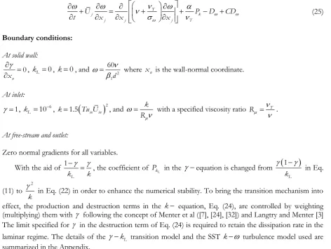
t x x x (25)

Boundary conditions:

At solid wall: 

 

x_n 0, kL 0, k0, and

 



 ₂

1 60

d where xn is the wall-normal coordinate.

At inlet:

 1, kL 106, 





2

1.5 _{in in}

k Tu U , and

 



 k

R with a specified viscosity ratio 

 

 T R .

At free-stream and outlet:

Zero normal gradients for all variables.

With the aid of 1 

L

k k, the coefficient of PkL in the



equation is changed from





 1

L

k in Eq.

(11) to 2

k in Eq. (22) in order to enhance the numerical stability. To bring the transition mechanism into

effect, the production and destruction terms in the k equation, Eq. (24), are controlled by weighting (multiplying) them with



following the concept of Menter et al ([7], [24], [32]) and Langtry and Menter [3] The limit specified for



in the destruction term of Eq. (24) is required to retain the dissipation rate in the laminar regime. The details of the



kL transition model and the SST k



turbulence model used are

summarized in the Appendix.

3.

Model Implementation and Numerical Method

The  equation in Eq. (22), the k_L equation in Eq. (23), and the SST k turbulence model in Eqs. (24) - (25) are implemented into the commercial CFD software ANSYS FLUENT version 14.0 by transforming these model transport equations into the User-Defined Scalar (UDS) transport equations in

User-Defined Functions (UDFs) as guided in the ANSYS FLUENT UDF manual, including _T in Eq. (20)

and T, in Eq. (21) that are added into the momentum equations in Eq. (19) via the diffusion term using

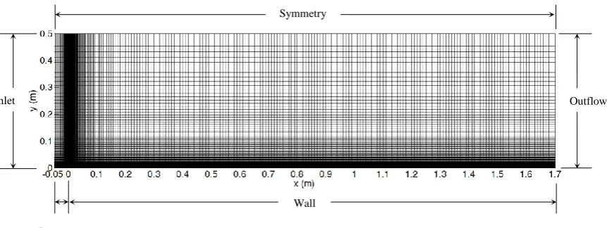
the built-in DEFINE_TURBULENT_VISCOSITY macro and the source term using the built-in DEFINE_SOURCE macro respectively. The implementation of the models into ANSYS FLUENT using UDF is properly validated. The SIMPLEC scheme is selected to cope with the pressure-velocity coupling. The second-order upwind scheme is used for the discretization in all equations. In case of the transitional boundary layer on a flat plate with zero pressure gradient, the mesh resolution and number of cells used for the ERCOFTAC test cases T3AM, T3A and T3B are summarized in Table 1, and a typical mesh distribution is shown in Fig. 1 where the domain inlet is located at the streamwise distance x 0.05 m upstream of the leading edge (x0m).

Table 1. Mesh and cell information for the transitional boundary layers on a flat plate with zero pressure gradient.

Test case Mesh resolution in x direction Mesh resolution in y direction No. of cells

T3AM 794 176 138775

T3A 336 147 48910

[image:9.595.65.538.82.437.2]

Fig. 1. Computational domain, boundary conditions and mesh distribution for the transitional boundary layer on a flat plate with zero pressure gradient.

In case of the transitional boundary layer on a flat plate with non-zero pressure gradient, the mesh resolution employed for the ERCOFTAC test cases T3C1-T3C5 is 300 75x in the streamwise and wall-normal directions respectively, and a typical mesh distribution is displayed in Fig. 2.

Fig. 2. Computational domain, boundary conditions and mesh distribution for the transitional boundary layer on a flat plate with non-zero pressure gradient.

In case of the transitional flow in a compressor cascade of Zaki et al [5], the mesh resolution is 223 226x in the streamwise and wall-normal directions respectively, and a typical mesh distribution is illustrated in Fig. 3. For all simulations, the first cell center adjacent to the wall is maintained to locate well below the distance of y 1. All the results presented here are grid-independent solutions.

Symmetry

Outflow Inlet

Wall Symmetry

Slip

Inlet

[image:10.595.91.522.89.251.2] [image:10.595.87.519.358.520.2]

Fig. 3. Computational domain, boundary conditions and mesh distribution for the transitional flow in a compressor cascade. Only every third line in x- and y-directions is presented in the mesh distribution.

4.

Results and Discussion

The  k_L transition model is validated with the experimental data of Coupland [1] in ERCOFTAC T3

series (T3AM, T3A, T3B) in case of the transitional boundary layer on a flat plate with zero pressure gradient and the experimental data of Coupland [1] in ERCOFTAC T3C series (T3C1-T3C5) in case of the transitional boundary layer on a flat plate with non-zero pressure gradient. The performance of the  k_L

transition model is assessed in case of the transitional flow in a compressor cascade where the DNS data of Zaki et al [5] are available. The predicted results of (1) flow with zero pressure gradient, (2) flow with non-zero pressure gradient, and (3) flow in a compressor cascade are summarized in Subsections 4.1, 4.2 and 4.3 respectively. Discussion on model performance is given in Subsection 4.4. In comparison with the results of the  k_L transition model, the results from the kL and



Re transition models are obtained from

ANSYS FLUENT which are already validated with the original ones reported in Walters and Cokljat [2] and Langtry and Menter [3] respectively.

4.1. Flow with Zero Pressure Gradient

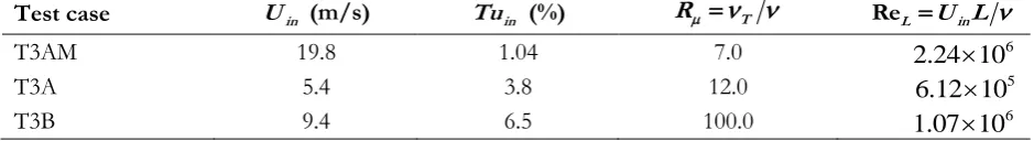
The computational domain and boundary conditions are shown in Fig. 1. The inlet conditions of T3AM, T3A and T3B are summarized in Table 2 where the free-stream velocity at inlet Uin is fixed with the same

value as given in the experimental data while the free-stream turbulence intensity at inlet Tu_in and the viscosity ratio at inlet R are adjusted to match the decay of free-stream turbulence intensity between

simulation and experiment. Only the  k_L transition model is considered in this case.

Table 2. Inlet conditions for ERCOFTAC T3 series where L = 1.7 m is the length of the flat plate.

Test case Uin (m/s) Tuin (%) R  T ReL U Lin 

T3AM 19.8 1.04 7.0 6

2.24 10

T3A 5.4 3.8 12.0 5

6.12 10

T3B 9.4 6.5 100.0 6

1.07 10

Figure 4 shows the decay of free-stream turbulence intensity, Tu, where the simulation results fit the experimental data very well for all three test cases.

Suction-side wall Periodic

42° Inlet

Outflo w

Periodic

Uin

[image:11.595.61.519.57.281.2] [image:11.595.63.533.655.719.2]

Fig. 4. Decay of free-stream turbulence intensity in case of the transitional boundary layer on a flat plate with zero pressure gradient. Lines for simulations. Symbols for experimental data.

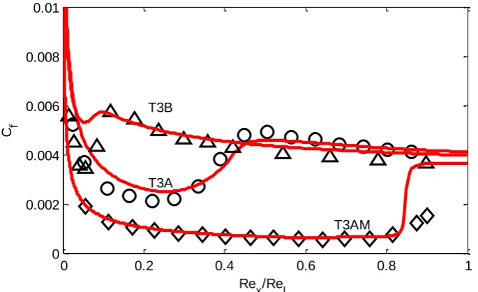
In Fig. 5, the distributions of skin friction coefficient, Cf , obtained from the simulations are in good

agreement with the experimental data for T3A and T3AM test cases. For T3B test case, the  k_L

transition model cannot capture the minimum value of Cf .

Fig. 5. Distribution of Cf in case of the transitional boundary layer on a flat plate with zero pressure

gradient. Lines for simulations. Symbols for experimental data.

4.2. Flow with Non-Zero Pressure Gradient

In this case, the computational domain and boundary conditions are shown in Fig. 2. The local height of the upper curved boundary from the lower flat plate is mathematically described following the conservation law of mass so that the local free-stream velocity as a slip boundary condition is distributed in the same way as the experimental data, and hence the desired pressure gradient is obtained. The formulations of the local

0 0.2 0.4 0.6 0.8 1

0 1 2 3 4 5 6

T3B

T3A

T3AM

Re_x/Re_L

Tu



(

%

)

0 0.2 0.4 0.6 0.8 1

0 0.002 0.004 0.006 0.008 0.01

T3B

T3A

T3AM

Re_x/Re_L

[image:12.595.135.454.100.311.2] [image:12.595.123.466.431.640.2]





 6 5 4 3 2 

/ min 1.356 7.591 16.513 17.510 9.486 2.657 0.991,1

h H x x x x x x (26a)





 6 5 4 3 2 

/ min 1.231 6.705 14.061 14.113 7.109 1.900 0.950,1

h H x x x x x x (26b)

where h is the local height of the upper curved boundary, H is the height of the upper curved boundary at inlet (H0.2m), and x is the streamwise distance along a lower flat plate starting from the leading edge (

0

x m). Eq. (26a) is specifically applied to T3C4 while Eq. (26b) is applied to T3C1, T3C2, T3C3 and

T3C5. Figure 2 displays a typical profile of the upper curved boundary.

The inlet stream velocity conditions of T3C1-T3C5 are summarized in Table 3 where the free-stream velocity at inlet Uin is adjusted to match the local free-stream velocity distribution between the

[image:13.595.158.437.324.405.2]

simulation results and the experimental data. In this case, the  k_L transition model is considered in comparison with the k_L and



Re transition models within the same CFD software.

Table 3. Inlet free-stream velocity conditions for ERCOFTAC T3C series where L is the horizontal length

of the upper curved boundary from the leading edge x = 0 m to x = 1.7 m.

Test case

Uin

(m/s)

ReL U Lin 

T3C1 5.7 6.46x105

T3C2 4.85 5.50x105

T3C3 3.55 4.02x105

T3C4 1.14 1.29x105

T3C5 8.2 9.29x105

It is shown in Fig. 6 that the distributions of the local free-stream velocity obtained from the simulations of T3C1-T3C5 are in good agreement with the experimental data for all three transition models.

Fig. 6. Distribution of the local free-stream velocity in case of the transitional boundary layer on a flat plate with non-zero pressure gradient.

In Table 4 and Table 5, the inlet free-stream turbulence intensity and viscosity ratio conditions of T3C1-T3C5 are summarized respectively where the free-stream turbulence intensity at inlet Tu_in and the

0 0.2 0.4 0.6 0.8 1 1.2 1.4 1.6 2

4 6 8 10 12 14

T3C1

T3C2

T3C3

T3C4 T3C5

x

U

Exp

-k

[image:13.595.212.381.467.682.2]

viscosity ratio at inlet R_ of each transition model are adjusted to match the decay of free-stream

turbulence intensity between the simulation results and the experimental data.

Table 4. Inlet free-stream turbulence intensity conditions for ERCOFTAC T3C series.

Test case Tuin (%)

L

k

   Re kL

T3C1 15.0 15.0 15.0

T3C2 5.0 5.0 5.0

T3C3 4.0 4.0 4.5

T3C4 3.0 4.0 3.0

T3C5 5.0 7.0 5.0

Table 5. Inlet viscosity ratio conditions for ERCOFTAC T3C series.

Test case R  T

L

k

   Re kL

T3C1 60.0 60.0 55.0

T3C2 9.0 9.0 9.0

T3C3 7.0 7.0 7.5

T3C4 3.0 4.0 4.0

T3C5 16.0 20.0 16.0

Figure 7 shows the decay of free-stream turbulence intensity where the simulation results obtained from all three transition models can fit the experiment data for all five test cases.

Fig. 7. Decay of free-stream turbulence intensity in case of the transitional boundary layer on a flat plate with non-zero pressure gradient.

For the T3C1 test case, the distribution of Cf is shown in Fig. 8 where the kL transition model can

predict the minimum value of Cf very well while both  kL and  Re transition models over-predict

0 0.2 0.4 0.6 0.8 1 1.2 1.4

0 1 2 3

T3C5

Re_x/Re_L T3C5 T3C5

0 0.2 0.4 0.6 0.8 1 1.2 1.4

0.5 1 1.5 2 2.5 3

T3C4 T3C4 T3C4

0 0.2 0.4 0.6 0.8 1 1.2 1.4

0.5 1 1.5 2 2.5 3

T3C3

Tu



(

%

)

T3C3 T3C3

0 0.2 0.4 0.6 0.8 1 1.2 1.4

0.5 1 1.5 2 2.5 3

T3C2 T3C2 T3C2

0 0.2 0.4 0.6 0.8 1 1.2 1.4

2 4 6 8

[image:14.595.139.456.149.244.2] [image:14.595.139.458.282.377.2] [image:14.595.236.392.426.679.2]

the minimum value of Cf . The onset of transition is well predicted by all three transition models but the

transition lengths from these three transition models are rather short compared to the experimental data.

Fig. 8. Distribution of Cf in case of T3C1.

The distribution of Cf in case of T3C2 is illustrated in Fig. 9 in which the predicted result of the  k_L transition model is in good agreement with the experimental data whereas both Re and  kL

transition models similarly predict the delayed onset of transition and hence the under-predicted distribution of Cf in the transition zone.

Fig. 9. Distribution of Cf in case of T3C2.

0 1 2 3 4 5 6 7 8

x 105 0

0.002 0.004 0.006 0.008 0.01

Re_x

C f

Exp -k_L -Re_

k_L

0 1 2 3 4 5 6 7

x 105 0

0.002 0.004 0.006 0.008 0.01

Re_x

C f

Exp -k_L -Re_

[image:15.595.115.454.137.347.2] [image:15.595.113.454.467.680.2]

In case of T3C3 where the distribution of Cf is displayed in Fig. 10, the predicted result of the  kL

[image:16.595.114.455.144.358.2]

transition model is in good agreement with the experimental data while the  Re transition model yields  too fast growth rate for Cf and the kL transition model predicts the onset of transition too late.

Fig. 10. Distribution of Cf in case of T3C3.

[image:16.595.114.456.473.692.2]

For the T3C4 test case, the distribution of Cf is shown in Fig. 11 where the predicted result of the  k_L transition model is in reasonably good agreement with the experimental data. The  Re  transition model predicts the good onset location of transition but the transition growth rate is too slow. Like the T3C3 test case, the k_L transition model predicts the onset of transition too late in this case.

Fig. 11. Distribution of Cf in case of T3C4.

Figure 12 illustrates the distribution of Cf in case of T3C5 in which the predicted result of the  kL

transition model is in good agreement with the experimental data. The Re transition model under- predicts the distribution of C in the transition zone due to the slightly delayed onset of transition. Similar

0 1 2 3 4 5

x 105 0

0.002 0.004 0.006 0.008 0.01

Re_x

C f

Exp -k_L -Re_

k_L

0 0.5 1 1.5 2

x 105 0

0.002 0.004 0.006 0.008 0.01

Re_x

C f

Exp -k_L -Re_

to the T3C3 and T3C4 test cases, the kL transition model predicts the onset of transition too late in this

[image:17.595.114.457.121.331.2]

case.

Fig. 12. Distribution of Cf in case of T3C5.

4.3. Flow in a Compressor Cascade

The geometry of the compressor blade is based on NACA 65. The computational domain and boundary conditions are shown in Fig. 3. The inflow angle of the inlet free-stream velocity is 42o _{with respect to the}

horizontal axis. The inlet conditions of T2 and T3 test cases are summarized in Table 6.

Table 6. Inlet conditions for flow in a compressor cascade where

L

is the axial chord length.

Test case Uin (m/s) Tuin (%) kin in ReL U Lin 

T2 2.0775 9.0 0.05243948 130.0 138500

T3 2.0775 11.0 0.07833551 100.0 138500

In this case, the computational domain, mesh and inlet conditions are adopted from Ge et al [4]. Since all three transition models ( k_L,  Re and  kL models) are applied with the same computational

domain, mesh and inlet conditions as Ge et al [4] so that the performance of these three transition models can be compared with that of the  transition model of Ge et al [4]. With the same inlet conditions, the computed results of the decay of turbulence intensity along the mid-pitch obtained from the  k_L,



 _{Re and} k_L transition models are compared with the DNS data of Zaki et al [5] for both T2 and T3

test cases in Fig. 13 in which the results of both  k_L and  Re transition models are in good  agreement with the DNS data while the results of the kL transition model are under-predicted for both T2

and T3 test cases. This implies that the k_L transition model is sensitive to the inlet conditions. For the T2 test case, the distributions of Cf along the suction- and pressure-side surfaces of the compressor blade are

shown in Fig. 14 and Fig. 15 respectively. On the suction-side surface, there appears a separation bubble in the DNS data which can be detected by the  k_L, kL and  transition models whereas the  Re 

transition model cannot detect the separation. The separation lengths predicted by the k_L, k_L and 

transition models are almost the same but larger than that of the DNS data. It is noticed that in this T2 case the  k_L transition model fails to predict reattachment. The reattachment cannot be captured because the energy transfer from the laminar kinetic energy (k_{L) to the turbulent kinetic energy (}k) is insufficient.

0 2 4 6 8 10 12

x 105 0

0.002 0.004 0.006 0.008 0.01

Re_x

C f

Exp -k_L -Re_

[image:17.595.64.528.468.509.2]

The minimum value of Cf in the DNS data can be best predicted by the  transition model but worst by

the k_L transition model. On the pressure-side surface, there is no separation bubble in the DNS data which can be predicted correctly by the  k_L, Re and  transition models, except the kL transition

model which predicts a large extent of separation zone. The minimum value of Cf in the DNS data can be

predicted correctly by the  Re and   transition models but is over-predicted by the  kL transition

[image:18.595.131.454.219.425.2]

model. The onset of transition can be predicted correctly by the  k_L and  Re transition models but  is delayed as found in the result of the  transition model.

Fig. 13. Decay of turbulence intensity along the mid-pitch in case of the transitional flow in a compressor cascade (T2 and T3 test cases).

Fig. 14. Distribution of Cf on the suction-side surface in case of T2.

-0.50 0 0.5 1 1.5

2 4 6 8 10

T2 T3

x/L

T

u

(

%

)

DNS

-k

L -Re_ k

L

0 0.2 0.4 0.6 0.8 1

-0.005 0.000 0.005 0.010 0.015

x/L

C f

DNS -k

L

-Re_ k

L

[image:18.595.116.457.480.687.2]

[image:19.595.115.456.92.299.2]

Fig. 15. Distribution of Cf on the pressure-side surface in case of T2.

The distributions of the pressure coefficient, C_P, along the suction- and pressure-side surfaces of the compressor blade are shown in Fig. 16. On the pressure-side surface, the  k_L , Re and   transition models can predict the distribution of C_P very well, except the k_L transition model. On the suction-side surface, there is a dip in the DNS data at around x L/ 0.6 which can be correctly predicted only by the  k_L transition model while over-predicted by the  Re and  transition models and under-predicted by the k_L transition model.

Fig. 16. Distribution of CP in case of T2.

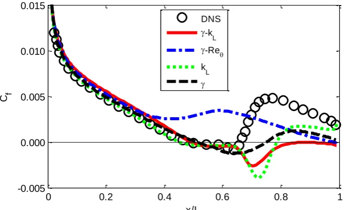
For the T3 test case, the distributions of Cf along the suction- and pressure-side surfaces of the

compressor blade are shown in Fig. 17 and Fig. 18 respectively. On both suction- and pressure-side surfaces, there is no separation bubble detected in the DNS data. However, the k_L transition model detects the fault separation bubble on both suction and pressure sides. On the suction-side surface, the  k_L

transition model can predict the Cf distribution better than the  Re and   transition models where

0 0.2 0.4 0.6 0.8 1

-0.005 0.000 0.005 0.010 0.015

x/L

C f

DNS -k

L

-Re_ k

L



0.2 0.4 0.6 0.8 1

-0.4 -0.2 0 0.2 0.4 0.6

x/L

C P

[image:19.595.122.448.452.664.2]

the  Re transition model over-predicts the  Cf distribution in the transition region while the 

transition model predicts the fault separation like the k_L transition model. On the pressure-side surface, the  k_L, Re and  transition models can reasonably predict the Cf distribution in the transition

region. The minimum value of Cf in the DNS data can be best predicted by the  transition model but

worst by the  k_L transition model. It is noticed that the transition extent in this T3 case predicted by the

[image:20.595.114.453.207.415.2]

 k_Ltransition model is rather small on both suction- and pressure-side surfaces.

Fig. 17. Distribution of Cf on the suction-side surface in case of T3.

Fig. 18. Distribution of Cf on the pressure-side surface in case of T3.

The distributions of CP along the suction- and pressure-side surfaces of the compressor blade are

shown in Fig. 19 in which the k_L,Re and  transition models can predict the distribution of CP

very well, except the k_L transition model which detects the fault dips of C_P on both suction and pressure sides.

0 0.2 0.4 0.6 0.8 1

-0.005 0.000 0.005 0.010 0.015

x/L

C f

DNS -k

L

-Re_ k

L



0 0.2 0.4 0.6 0.8 1

-0.005 0.000 0.005 0.010 0.015

x/L

C f

DNS -k

L

-Re_ k

L

[image:20.595.116.453.446.659.2]

[image:21.595.127.447.88.304.2]

Fig. 19. Distribution of C_P in case of T3.

4.4. Discussion on Model Performance

The DNS data of the transitional flow in the compressor cascade from Zaki et al [5] is a good test case for assessing the performance of transition models because the ERCOFTAC T3- and T3C-series experimental data have already been employed to determine the appropriate values for the model constants. The ability to detect a separation bubble on a compressor blade is a good indicator for the prediction capability of transition models. Therefore, the separation bubbles detected on the suction- and pressure-side surfaces of the compressor blade by the  Re ,  kL,  and  kL transition models are summarized in comparison

with the DNS data in Table 7. It is found that the  k_L transition model is the one and only transition model that can consistently predict the existence of the separation bubble on the compressor blade.

Table 7. Summary of model performance.

Transition models T2 test case T3 test case

Suction side Pressure side Suction side Pressure side

DNS separation no separation no separation no separation

 k_L separation no separation no separation no separation



 Re no separation no separation no separation no separation

L

k separation separation separation separation

 _{separation no separation separation no separation}

5.

Conclusion

The present research work has been conducted in order to continually develop and propose a new and complete version of the  k_L transition model that can apply to the transitional flow with pressure

gradient. The new  k_L transition model is validated with the ERCOFTAC T3- and T3C-series

experimental data of Coupland [1]. The validated results of the  k_L transition model are in good agreement with the experimental data. The performance of the  k_L transition model is assessed in case of the transitional flow through the compressor blade passage of Zaki et al [5]. It is found that the  k_L

transition model is the only transition model that can consistently capture the separation bubble on the compressor blade.

0.2 0.4 0.6 0.8 1

-0.4 -0.2 0 0.2 0.4 0.6

x/L

C P

DNS -k

L

-Re_ k

L

[image:21.595.65.537.500.613.2]

Acknowledgements

The authors would like to gratefully thank Dr. Rodolphe Perrin for his valuable discussion during his visit to TGGS at KMUTNB on 11 May – 25 July 2015 with the KMUTNB financial support, Dr. Tamer Zaki for his DNS data of the transition in a compressor cascade, and Mr. Xuan Ge for his RANS results of the transition in a compressor cascade.

Appendix: Details of the





k

_L

Transition Model and the SST

k





Turbulence Model

Used

All physical terms, extra term, parameters, functions and constants of the  k_L transition model are given below:

Production terms:



 2

k T

P S



 2

,

L

k T

P S

Destruction terms:

 

 *

k

D k

 2 D

 



 

2 L L

L

j j

k k D

x x

Redistribution terms:



 , 

NAT R NAT NAT L

R C k

 

 R BP, BP

BP L

W C

R k

f

Other relevant physical terms:

 2 _{ij ij}

S S S = Magnitude of the mean strain rate

  

 _  _

 

 

1 2

j i ij

j i

U U S

x x = Mean strain rate

  2 _{ij ij} = Magnitude of the mean rotation rate

  

  _  _

 

 

1 2

j i ij

j i

U U

x x = Mean rotation rate





  

, 1

T SS W

k f f k= Large-scale turbulent kinetic energy







_eff min C d,_T = Effective length scale

 



 _*T T

k = Turbulent length scale

Parameters of the  k_L transition model:





 _{ } _  _     2 ,

max Re ,0

1 exp TS crit

TS TS C A     _ _  

1 exp NAT

NAT NAT A       _  _       , ,

max Re NAT crit ,0

NAT NAT crit C f     _ _  

1 exp BP

BP BP A       _  _{ }     ,  max ,0

BP BP crit

k _C

Functions of the  k_L transition model:

  _{ }   __{  }       2 exp SS SS f C k   _            ,

, 1 exp , 2 2

T eff k f C    eff W T f       _ _  

, 1 exp

L

NAT crit NC

k d

f C

Constants of the  kL transition model:

Model constants Specified values References

1. CNAT crit, 817 present

2. CBP crit, 8.2 present

3. C 0.39 present

4. CR NAT, 2 Juntasaro and Ngiamsoongnirn [31]

5. C 2 10-8 Juntasaro and Ngiamsoongnirn [31]

6. CR BP, 0.36 Juntasaro and Ngiamsoongnirn [31]

7. CSS CSS CBP crit2 , Juntasaro and Ngiamsoongnirn [31]

8. ABP 0.6 Walters and Cokjlat [2]

9. A_NAT 200 Walters and Cokjlat [2]

10. ATS 200 Walters and Cokjlat [2]

11. C_NC 0.1 Walters and Cokjlat [2]

12. CTS crit, 1000 Walters and Cokjlat [2]

13. C 1 3.4x10-6 Walters and Cokjlat [2]

Extra term and relevant functions of the SST k  turbulence model:





          1 2 1 2 1 j j k CD F x x







1 max 1,org, 3

F F F

 

 2

2 tanh arg2 F

 

 4

1,org tanh arg1 F                      

1 2 2

2

500 4

arg min max , ,

0.09 k

k k

d d CD d           2 2 2 500

arg max ,

0.09 k d d        _{ }   _ _     20 2 1

max 2 ,10

k j j k CD x x  _{ }   _{ }        8 3 exp 120 y R F

Constants of the SST k  turbulence model:



1 0.31

a





F_{1 1}  1 F₁ ₂

where  stands for k, ,  and  with the following two-layer parts:

₁ (SST inner):_k11.176, 12.0 , 10.075 ,  

* _{0.09 ,  }

1 0.553

₂ (Standard k outer): _k21.0, 21.168 , 20.0828 ,  

* _{0.09 ,  }

2 0.44 Reynolds numbers:     2 Re d   y d k R

References

[1] J. Coupland. (1990). ERCOFTAC classic database. [Online]. Available:

http://cfd.mace.manchester.ac.uk/ercoftac/, Accessed on: 10 May 2005.

[2] D. K. Walters and D. Cokljat, “A three-equation eddy-viscosity model for Reynolds Averaged Navier-Stokes simulations of transitional flow,” ASME Journal of Fluids Engineering, vol. 130, 2008.

[3] R. B. Langtry and F. R. Menter, “Correlation-based transition modeling for unstructured parallelized computational fluid dynamics codes,” Journal of American Institute of Aeronautics and Astronautics, vol. 47, no. 12, pp. 2894-2906, 2009.