Perturbation Observer based Adaptive Passive Control and Applications for VSC-HVDC Systems and FACTS Devices

(1)

Perturbation Observer based Adaptive Passive Control and

Applications for VSC-HVDC Systems and FACTS Devices

Thesis submitted in accordance with the requirements of the University of Liverpool

for the degree of Doctor of Philosophy

in

Electrical Engineering and Electronics

by

Bo Yang, B.Sc.(Eng.)

(2)

Perturbation Observer based Adaptive Passive Control and Applications for VSC-HVDC Systems and FACTS Devices

by Bo Yang

(3)

I would like to give my heartfelt thanks to my primary supervisor, Dr. L. Jiang, whose encouragement, guidance and support enabled me to develop a deep under-standing of my work. Without his consistent and illuminating instructions, my re-search work and my life could not proceed to this stage. The rere-search skill, writing skill and presenting skill he taught me will benefit me throughout my life.

I would like to show my gratitude to my secondary supervisor, Professor Q. H. Wu, for his kind guidance with his knowledge of control and power systems, and his inspiring insight into life philosophy, piano, and poetry.

I offer my regards and blessings to all of the members of Smart Grid Control and Renewable Energy Group, the University of Liverpool, especially to Dr. W. Yao for his kind and helpful discussion on power system modelling and operation, Dr. C. K. Zhang for his expert control knowledge, and Mr. S. Kai for his excellent hardware experiment skill. Special thanks also go to my friends, Mr. Nick Liu, Mr. Z. H. Fang, and Dr. Simon for their consistent support and friendship, which made my life in U. K. so wonderful.

I am grateful to the Department of Electrical Engineering and Electronics at the University of Liverpool, for providing the research facilities that made it possible for me to carry out this research. I am indebted to the University of Liverpool for the studentship (2011-2015), and China Scholarship Council (CSC) (2011-2015) for the financial support.

Finally, I am greatly thankful to my father Z. H. Yang and my mother P. L. Yang, for their encouragement and love for my whole life.

(4)

Abstract

The technology of voltage source converter based high voltage direct current (VSC-HVDC) system and devices used in flexible AC transmission systems (FACTS) has evolved significantly over the past two decades. It is used to effectively enhance power system stability. One of the important issues is how to design an applica-ble nonlinear adaptive controller for these devices to effectively handle the system nonlinearities and uncertainties.

Passive control (PC) has been proposed for the control of nonlinear systems based on Lyapunov theory, which has the potential to improve the system damping as the beneficial system nonlinearities are remained instead of being fully cancelled. However, PC is not applicable in practice as it requires an accurate system model. Adaptive passive control (APC) and robust passive control (RPC) have been devel-oped to handle some specific type of system uncertainties based on strict assump-tions on system structure and uncertainty. However, their applicaassump-tions are limited as various system uncertainties exist.

This thesis aims to develop a perturbation observer based adaptive passive con-trol (POAPC) to make PC applicable in practice. The combinatorial effect of system nonlinearities, parameter uncertainties, unmodelled dynamics and time-varying ex-ternal disturbances is aggregated into a perturbation, which is estimated by a pertur-bation observer (PO). The proposed approach does not require an accurate system model and can handle various system uncertainties.

POAPC is applied to two-terminal VSC-HVDC systems to handle various sys-tem uncertainties. The VSC-HVDC syssys-tem model is firstly developed, the proposed controller can inject an extra system damping and only the measurement of direct current (DC) voltage, active and reactive power is needed. The effectiveness of

(5)

out to verify its implementation feasibility and applicability.

A passive controller is designed for multi-terminal VSC-HVDC (VSC-MTDC) systems via energy shaping, in which the dynamics related to the active power, reac-tive power, and DC cable voltage is transformed into an output strictly passive form. Then the remained internal dynamics related to DC cable current and common DC voltage is proved to be asymptotically stable in the context of Lyapunov criterion. PC is applied on a four-terminal VSC-MTDC system under eight cases to evaluate its control performance.

POAPC is developed on the VSC-MTDC system to maintain a consistent control performance under different operating points and provide a significant robustness to parameter uncertainties, together with other unmodelled dynamics and time-varying external disturbances. Simulation results are provided to evaluate the control per-formance of POAPC in comparison to that of PI control and PC.

Perturbation observer based coordinated adaptive passive control (POCAPC) is proposed for excitation controller (EC) and FACTS controller on both single ma-chine infinite bus (SMIB) systems and multi-mama-chine power systems. Only the range of control Lyapunov function (CLF) is needed and the dependence of an ac-curate system model can be partially reduced, thus POCAPC can be easily applied to multi-machine power systems. Its control performance is compared with that of conventional proportional-integral-derivative and lead-lag (PID+LL) control, coor-dinated passive control (CPC) and coorcoor-dinated adaptive passive control (CAPC) on both an SMIB system and a three-machine power system by simulation. Then a hardware-in-the-loop (HIL) test is undertaken to verify the implementation feasibil-ity of the proposed controller.

(6)

Declaration

The author hereby declares that this thesis is a record of work carried out in the Department of Electrical Engineering and Electronics at the University of Liverpool during the period from October 2011 to September 2015. The thesis is original in content except where otherwise indicated.

(7)

List of Figures x

List of Tables xiii

1 Introduction 1

1.1 Background . . . 1

1.1.1 VSC-HVDC systems . . . 1

1.1.2 FACTS devices . . . 11

1.1.3 Passive control . . . 14

1.2 Motivation and Methodology . . . 16

1.3 Main Contributions . . . 17

1.4 Publication List . . . 19

1.5 Thesis Outline . . . 20

2 Perturbation Observer based Adaptive Passive Control 23 2.1 Introduction . . . 23

2.2 Problem Formulation . . . 26

2.3 Design and Stability Analysis of POAPC . . . 27

2.4 Case Studies . . . 35

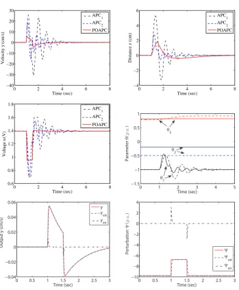
2.4.1 Magnetic levitator system . . . 35

2.4.2 Interconnected inverted pendulum system . . . 41

2.5 Conclusion . . . 43

3 Perturbation Observer based Adaptive Passive Control for Two-terminal VSC-HVDC Systems 47 3.1 Introduction . . . 47

3.3 Two-terminal VSC-HVDC System Modelling . . . 53

3.4 POAPC Design for Two-terminal VSC-HVDC System . . . 55

3.4.1 Rectifier controller design . . . 55

3.4.2 Inverter controller design . . . 57

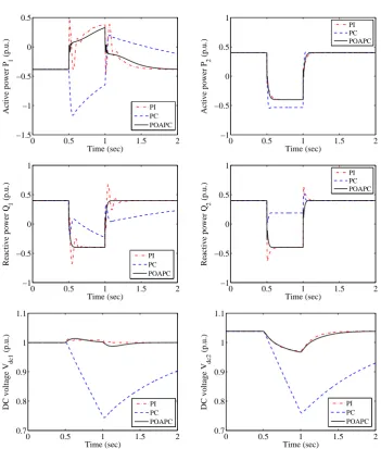
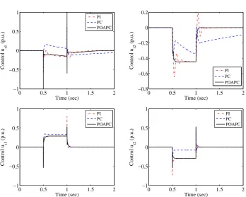
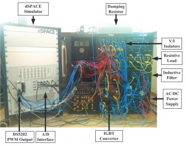
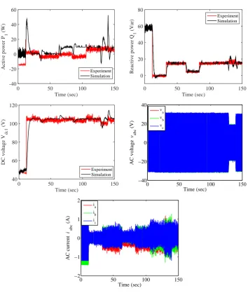
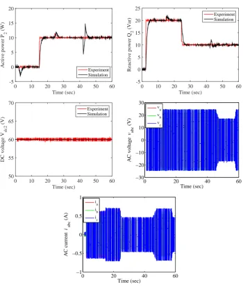
3.5 Simulation Results for Two-terminal VSC-HVDC System . . . 59 3.6 Experiment Results for Rectifier Controller and Inverter Controller . 66

(8)

3.6.1 Experiment platform . . . 67

3.6.2 Case studies . . . 70

4 Passive Control Design for VSC-MTDC Systems via Energy Shaping 75 4.1 Introduction . . . 75

4.2 N-terminal VSC-MTDC System Modelling . . . 77

4.3 PC Design forN-terminal VSC-MTDC System . . . 80

4.3.3 Internal dynamics stability . . . 84

5 Perturbation Observer based Adaptive Passive Control for VSC-MTDC Systems 98 5.1 Introduction . . . 98

5.2 POAPC Design forN-terminal VSC-MTDC System . . . 99

6 Perturbation Observer based Coordinated Adaptive Passive Control for Multi-machine Power Systems with FACTS Devices 116 6.1 Introduction . . . 116

6.2.1 Design of HGSPO and HGPO . . . 119

6.2.2 Design of stabilizing controller and coordinated controller . 122 6.2.3 The closed-loop system stability . . . 125

6.3 Power System Modelling . . . 128

6.3.1 An SMIB system with a TCSC device . . . 128

6.3.2 A multi-machine power system with a TCSC device . . . . 129

6.4 POCAPC Design for Generator Excitor and TCSC Device . . . 130

6.4.1 Controller design for an SMIB system . . . 130

6.4.2 Controller design for a multi-machine power system . . . . 132

6.5.1 The SMIB system . . . 136

6.5.2 The three-machine power system . . . 143

6.6 Hardware-in-the-loop Test . . . 153

6.7 Discussion . . . 157

(9)

7.2 Future Studies . . . 161

A Basic Concepts of Passive Systems 163

References 168

(10)

List of Figures

1.1 HVDC system based on CSC technology built with thyristors. . . . 3

1.2 HVDC system based on VSC technology built with IGBTs. . . 3

1.3 Conventional three-phase two-level VSC topology. . . 5

1.4 Two-level sinusoidal PWM method: reference (sinusoidal) and car-rier (triangular) signals and line-to-neutral voltage waveform. . . 6

1.5 Active-reactive locus diagram of VSC-based power transmission system with limitations. . . 6

2.1 Structure of the POAPC . . . 33

2.2 The magnetic levitator system. . . 36

2.3 System responses obtained under the nominal model. . . 37

2.4 System responses obtained under the unmodelled dynamics. . . 38

2.5 System responses obtained under the time-varying external distur-bance. . . 39

2.6 Two inverted pendulums on two carts. . . 40

2.7 System responses obtained under the nominal model. . . 44

2.8 System responses obtained under the unmodelled dynamics. . . 45

3.1 The two-terminal VSC-HVDC system . . . 54

3.2 Structure of the rectifier controller in two-terminal VSC-HVDC sys-tems. . . 57

3.3 Structure of the inverter controller in two-terminal VSC-HVDC sys-tems. . . 59

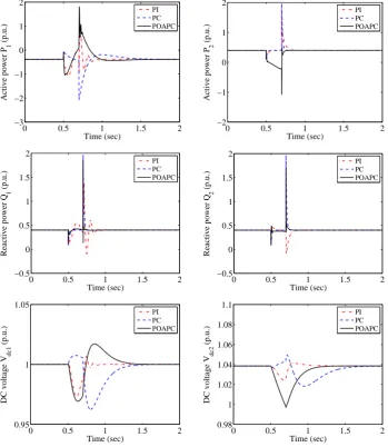
3.4 System responses obtained in an active and reactive power tracking. 62 3.5 System responses obtained in the voltage drop of AC grids. . . 63

3.6 System responses obtained under a 20% increase of system resis-tances and inducresis-tances. . . 64

3.7 Control efforts obtained under a 20% increase of system resistances and inductances. . . 65

3.8 Overall hardware platform. . . 66

3.9 Experiment configuration of Case I. . . 68

3.10 Experiment configuration of Case II. . . 69

3.11 The structure of an IGBT converter. . . 69

(11)

4.1 One terminal in anN-terminal VSC-MTDC system. . . 78

4.2 The topology of anN-terminal VSC-MTDC system. . . 79

4.3 Structure of PC for the VSC-MTDC system. . . 83

4.4 A four-terminal VSC-MTDC system. . . 87

4.5 System responses obtained in active and reactive power tracking. . . 88

4.6 System responses obtained under a 10-cycle LLLG fault at bus 1. . . 89

4.8 The overall storage function obtained under a 10-cycle LLLG fault at bus 1 and bus 4. . . 91

4.9 System responses obtained under a transmission line disconnection of AC network1and AC network4. . . 91

4.10 System responses obtained in a temporary DC cable1 fault. . . 92

4.11 System responses obtained when a modulated change occurs in the angular frequency. . . 93

4.12 System responses obtained under a 20% decrease of the system re-sistances and inductances. . . 94

4.13 System responses obtained when weak AC networks are connected. 95 4.14 System responses obtained with DC voltage measurement noises. . 96

5.1 Structure of the rectifier controller in VSC-MTDC systems. . . 100

5.2 Structure of the inverter controller in VSC-MTDC systems. . . 103

5.3 System responses obtained in active and reactive power tracking. . . 106

5.6 Estimation errors of HGSPO1 and HGPO1 obtained under a 10-cycle LLLG fault at bus 1. . . 108

5.7 System responses obtained under a transmission line disconnection of AC network1and AC network4. . . 109

5.8 System responses obtained in a temporary DC cable1 fault. . . 110

5.9 System responses obtained when a modulated change occurs in the angular frequency. . . 111

5.10 System responses obtained under a 20% decrease of the system re-sistances and inductances. . . 112

5.11 System responses obtained when weak AC networks are connected. 113 5.12 System responses obtained with DC voltage measurement noises. . 114

6.1 Structure of the stabilizing controlleru2. . . 123

6.2 Structure of the coordinated controlleru1. . . 124

6.3 The SMIB system equipped with a TCSC device. . . 129

6.4 Structure of conventional PID+LL controller. . . 137

(12)

6.5 System responses obtained with the EC alone, coordinated EC and TCSC controller, and approximated EC and TCSC controller in the SMIB system. . . 138 6.6 System responses obtained under the nominal model in the SMIB

system. . . 139 6.7 System responses obtained under an unmodelled TCSC dynamics

in the SMIB system. . . 141 6.8 System responses obtained under an inter-area type disturbance in

the SMIB system. . . 142 6.9 The three-machine power system equipped with a TCSC device. . . 143 6.10 System responses obtained under operation Type I and the nominal

model in the three-machine power system. . . 144 6.11 Estimation errors of HGSPO1for G1obtained under operation Type

I and the nominal model in the three-machine power system. . . 146 6.12 Estimation errors of HGPO for TCSC obtained under operation Type

I and the nominal model in the three-machine power system. . . 146 6.13 The effect of a 50% parameter increase on the dynamic response of

proposed controller without perturbation compensation obtained in the three-machine power system. . . 148 6.14 The effect of a 50% parameter increase on the dynamic response

of proposed controller with perturbation estimation obtained in the three-machine power system. . . 149 6.15 System responses obtained under operation Type I and the

parame-ter uncertainties in the three-machine power system. . . 150 6.16 System responses obtained under operation Type II and the

param-eter uncertainties in the three-machine power system. . . 151 6.17 The configuration of the HIL test. . . 154 6.18 The experiment platform of the HIL test. . . 154 6.19 System responses obtained in the HIL test with large observer poles

λ=λ′ = 15(fs= 50kHz,fc= 500Hz andτ = 2ms). . . 155

6.20 System responses obtained in the HIL test with proper observer polesλ =λ′ = 5(fs = 50kHz,fc = 500Hz andτ = 2ms). . . 156

(13)

1.1 Summary of fully controlled high power semiconductors [4] . . . . 2

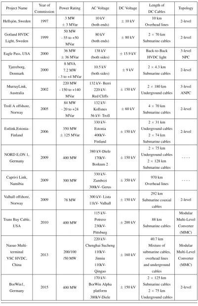
1.2 Summary of worldwide VSC-HVDC projects and their basic pa-rameters . . . 9

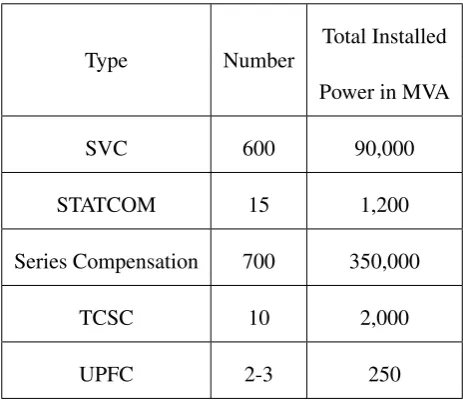
1.3 Estimated number of worldwide installed FACTS devices and their estimated total installed power . . . 13

3.1 System parameters used in the two-terminal VSC-HVDC system. . 60

3.2 Control parameters in the two-terminal VSC-HVDC systems. . . 60

3.3 System parameters used in Case I. . . 68

3.4 System parameters used in Case II. . . 68

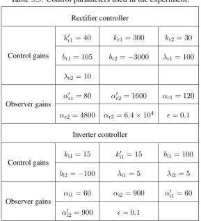
3.5 Control parameters used in the experiment. . . 73

4.1 System parameters used in the four-terminal VSC-MTDC system. . 87

5.1 Control parameters used in the four-terminal VSC-MTDC system. . 105

6.1 PID+LL control parameters of the SMIB system. . . 136

6.2 POCAPC parameters of the SMIB system. . . 140

6.3 SMIB system parameters (in p.u.). [56] . . . 140

6.4 PID+LL control parameters of the three-machine power system. . . 144

6.5 POCAPC parameters of the three-machine power system. . . 145

6.6 Three-machine power system transmission line parameters (in p.u.). [56] . . . 145

6.7 Three-machine power system operation Type I. . . 147

6.8 Three-machine power system operation Type II. . . 147

6.9 IAE index of different control schemes . . . 152

(14)

List of Abbreviations and Notations

Abbreviations in Control Systems

PC Passive control.

PO Perturbation observer. HGO High-gain observer.

HGPO High-gain perturbation observer.

HGSPO High-gain state and perturbation observer. FLC Feedback linearization control.

APC Adaptive passive control.

POAPC Perturbation observer based adaptive passive control. RPC Robust passive control.

CPC Coordinated passive control.

CAPC Coordinated adaptive passive control.

POCAPC Perturbation observer based coordinated adaptive passive control. PID Proportional-integral-derivative.

VC Vector control.

PI Proportional-integral. SMO Sliding-mode observer. SMC Sliding-mode control. TDC Time delay control.

ADP Adaptive dynamic programming.

ADRC Adaptive disturbance rejection controller. CLF Control Lyapunov function.

SISO Single-input single-output. MIMO Multi-input multi-output.

Abbreviations in VSC-HVDC Systems

(15)

HVDC High voltage direct current.

VSC-HVDC Voltage source converter based high voltage direct current.

VSC-MTDC Voltage source converter based multi-terminal high voltage direct current. HIL Hardware-in-the-loop.

IGBT Insulated gate bipolar transistor. PWM Pulse width modulation.

SPWM Sinusoidal pulse width modulation. SVM Space vector modulation.

PLL Phase-locked loop. AC Alternating current.

DC Direct current.

I/O Input/output.

A/D Analogue/digital.

SVPWM Space vector pulse width modulation.

Abbreviations in Power Systems

EC Excitation controller.

TCSC Thyristor controlled series capacitor.

FACTS Flexible alternating current transmission systems. SMIB Single machine infinite bus.

LL Lead-lag.

PSS Power system stabilizer. AVR Automatic voltage regulator. SVC Static VAR compensator.

STATCOM Static synchronous compensator.

p.u. Per unit.

Symbols

∀ for all.

∃ exist.

(16)

⇒ implies.

→ tends to.

7→ maps to.

∂ partial derivative.

∑

sum.

∈ in.

∞ infinity.

∠ angle.

lim limit.

max maximum.

min minimum.

sup supremum, the least upper bound.

inf infimum, the greatest lower bound.

min designation the end of proofs.

Rn _the_n_{-dimensional Euclidean space.}

Vectors and Matrices

|a| the absolute value of a scalara. ∥x∥p the inducedp-norm of vectorx, i.e.

∥x∥p = (|x1|p +· · ·+|xn|p)1/p,1≤p <∞;

∥x∥_∞= maxi|xi|.

∥x∥ the Euclidean norm of a vectorx, i.e.∥x∥= (xTx)1/2.

∥A∥p the inducedp-norm of a matrixA,

i.e.∥A∥p = supx̸=0 ∥

Ax∥p

∥x∥p .

∥A∥ the induced 2-norm of a matrixA, i.e.∥A∥= [λmax(ATA)]1/2.

diag[a1,· · · , an] a diagonal matrix with diagonal elementsa1 toan.

AT₍_xT₎ _{the transpose of a matrix}_A_{(a vector}_x_).

λmax(P)(λmin(P)) the maximum and (minimum) eigenvalues of a symmetric matrixP.

P >0(P ≥0) a positive definite (semi-definite) matrixP.

(17)

Introduction

1.1 Background

1.1.1 VSC-HVDC systems

(18)

1.1 Background 2

Table 1.1: Summary of fully controlled high power semiconductors [4]

Acronym Type Full Name

IGBT Transistor Insulated Gate Bipolar Transistor IEGT Transistor Injection Enhanced Gate Transistor GTO Thyristor Gate Turn-off Thyristor IGCT Thyristor Integrated Gate Commutated Thyristor

GCT Thyristor Gate Commutated Turn-off Thyristor

management of electrical power, which ensures the technology has a remarkably important role in the modern electrical power industry [4].

The ever increasing penetration of power electronics technologies into power systems mainly results from the continuous development of high voltage high power fully controlled semiconductors [5], which adopts different types of fully controlled semiconductor devices, such as thyristor or transistor based electronics shown in Table 1.1 [4]. These devices can be employed for a voltage source converter (VSC) with pulse width modulation (PWM) operating at a frequency higher than the line frequency. These devices are all self-commuted via a gate pulse [6]. Typically, it is desirable that a VSC generates PWM waveforms of higher frequency when compared to the thyristor-based systems. However, the operating frequency of these devices is also determined by the switching losses and the design of the heat sink, both of which are closely related to the power through the components. Switching losses, which are directly linked to high-frequency PWM operation, are one of the most serious and challenging issues that must be resolved by VSC-based high power applications [7]. Other obvious disadvantages are the electromagnetic compatibility or electromagnetic interference (EMC/EMI) and transformer insulation stresses [8, 9].

(19)

Grid1

vb1

va1

vc1

vb2

va2

vc2

Grid2

DC cable

DC cable Current

Direction

Figure 1.1: HVDC system based on CSC technology built with thyristors.

Grid1

vb1 va1

vc1

Vdc1 vb2

va2

vc2

Vdc2

+

-+

-Grid2 DC cable

DC cable

Figure 1.2: HVDC system based on VSC technology built with IGBTs.

• Line-commutated current source converters (CSCs) that use thyristors shown in Fig. 1.1. This technology is well established for high power, typically around 1000 MW, with the largest project being the Itaipu system in Brazil at 6300 MW power level. The longest power transmission in the world transmits 6400 MW power from the Xiangjiaba hydropower plant to Shanghai, which line length is 2071 km and will use 800 kV HVDC and 1000 kV ultrahigh-voltage AC transmission technology [10].

• Forced-commutated VSCs that use gate turn-off thyristors (GTOs) or in most industrial cases insulated gate bipolar transistors (IGBTs) illustrated in Fig. 1.2. It is a well-established technology for medium power levels with recent projects ranging around 300-400 MW power level [11].

(20)

1.1 Background 4

also referred to as the ‘classical’ HVDC system), and recently, a large number of significant advances have been achieved [12]. On the other hand, the VSC-HVDC systems represent latest developments in the area of DC power transmission technol-ogy [11]. The operation experience with VSC-HVDC system at commercial level scatters over the last two decades [11, 12]. The breakthrough was made when the world’s first VSC-based PWM-controlled HVDC system using IGBTs was installed in March 1997 (Hellsj¨on project, Sweden, 3 MW, 10 km distance, ±10 kV) [13]. Since then, more VSC-HVDC systems have been installed worldwide [14].

The CSCs have the natural ability to withstand short-circuit fault because the DC inductors can limit the currents when faults occur. In contrast, the VSCs are more vulnerable to line faults, hence cables are more attractive for VSC-HVDC ap-plications. It is worth mentioning that relevant developments, such as the advanced extruded DC cable technologies [15], can lead to the success of VSC-HVDC system. Furthermore, faults on the DC side of VSC-HVDC systems can also be addressed by using the DC circuit breakers (CBs) [16, 17]. In the event of the loss of a VSC in a multi-terminal HVDC (MTDC) system, the excess of power can be restricted by the advanced DC voltage controller [18].

A basic VSC-HVDC system comprising of two converters built with VSC topol-ogy is demonstrated by Fig. 1.2. The simplest VSC topoltopol-ogy is the conventional two-level three-phase bridge shown in Fig. 1.3. Typically, many series-connected IGBTs are used for each semiconductor as illustrated by Fig. 1.3, such that a higher blocking voltage capability for the converter can be delivered, and therefore increase the DC bus voltage level of the VSC-HVDC system. Note that an antiparallel diode is also required for the purpose of ensuring the four-quadrant operation of the con-verter. The DC bus capacitor provides the required storage of the energy so that the active and reactive power can be controlled and offers filtering for the DC harmon-ics.

(21)

vb va

vc S1

S4

S3

S6

S5

S2

D1 D3

Vdc _O

+

-+

-D5

D4 D6 D2

Figure 1.3: Conventional three-phase two-level VSC topology.

converter is connected through a reactor to the AC system. Filters are also included on the AC side to further reduce the harmonics flowing into the AC system.

Fig. 1.5 shows the entire active-reactive power area where the VSC can be op-erated with 1.0 per unit (p.u.) value being the megavolt amperes rating of each converter with limitations. The use of VSC as opposed to a line-commutated CSC offers the following advantages [4]:

• Avoidance of commutation failures due to disturbances in the AC network. • Independent control of the active and reactive power consumed or generated

by the converter.

• Possibility to connect the VSC-HVDC system to a weak AC network or even to one where no generation source is available, and naturally, the short-circuit level is very low.

• Faster dynamic response due to higher PWM than the fundamental switching frequency (phase-controlled) operation, which further results in reduced need for filtering, and hence smaller filter size.

• No need of transformers to assist the commutation process of the converter’s fully controlled semiconductors.

(22)

1.1 Background 6

Time 0

-1 p.u. 0 1 p.u. -1 p.u. 0 1 p.u.

Reference Fundamental

Carrier

Figure 1.4: Two-level sinusoidal PWM method: reference (sinusoidal) and carrier (triangular) signals and line-to-neutral voltage waveform.

-1.0

1.0

-1.0

1.0 Q [p.u.]

P [p.u.] 0.5

0.5 Over-voltage

Limitation

Under-voltage Limitation

Over-current Limitation

(23)

flow regulation in AC power systems, long-distance transmission, and introduction of the supergrid, which is a large-scale power grid interconnected between national power grids [20]. The VSC-HVDC system has been proposed for integration of long-distance large onshore wind farms via overhead line and offshore wind farms via submarine cable [18, 21].

One important issue that needs to be addressed carefully before the implemen-tation is the protection design of VSC-HVDC systems. Currently, many studies have been carried out to investigate the VSC-HVDC system protection as the whole system has to be isolated from the power system when the DC cable fault occurs. A transient harmonic current protection scheme is proposed in [22], in which the discrete Fourier transform was used to extract transient harmonic currents at both terminals of the DC transmission line and the type of fault can be identified by the transient harmonic currents. Based on the zero- and positive-sequence backward traveling waves, an integrated traveling wave-based protection scheme was devel-oped [23], which can detect faults rapidly, determine the fault type effectively, and select the faulty pole correctly. In addition, a transient energy protective scheme was developed [24] based on the distributed parameter line model, in which the transient energy distribution over the line can be obtained from the voltage and current measurements at both terminals and the fault can be recognized from the calculated value simply. Recently, an apparent impedance calculation method was proposed [25], which utilizes the bus impedance matrix to calculate the impedances viewed by distance relays during a three-phase SC fault. [26] proposed a whole-line quick-action protection principle for HVDC transmission lines, which is based on the boundary characteristics of the line, can distinguish internal faults from external ones using single-terminal current measurements only.

(24)

transmis-1.1 Background 8

sion capacity than that of AC networks and provides a more flexible, efficient trans-mission method. The main applications of VSC-MTDC systems include power ex-change among multi-points, connection between multiple asynchronous networks, and integration of scattered power plants like offshore renewable energy sources such as wind farms and solar plants [27]. Other application can be found in urban sub-transmission [28], oil and gas platforms [29], premium quality power parks [30], wind power transmission in Norway [21], and European supergrid [31]. Recently, the world’s first MTDC system employing VSC technology called Nanao’s VSC-MTDC project has been built in China [32]. Table 1.2 summarizes some worldwide VSC-HVDC projects [4, 33].

(25)

[image:25.595.106.508.113.734.2]

Table 1.2: Summary of worldwide VSC-HVDC projects and their basic parameters

Project Name Year of

Commission Power Rating AC Voltage DC Voltage

Length of

DC Cables Topology

Hellsj¨on, Sweden 1997 3 MW

±3 MVar

10 kV

(both ends) ±10 kV

10 km

Overhead lines 2-level

Gotland HVDC

Light, Sweden 1999

50 MW

- 55 to +50

MVar

80 kV

(both ends) ±80 kV

2×70 km

Submarine cables 2-level

Eagle Pass, USA 2000 36 MW

±36 MVar

138 kV

(both sides) ±15.9 kV

Back-to-Back HVDC light 3-level NPC Tjæreborg, Denmark 2000 8 MVA 7.2 MW

- 3 to +4 MVar

10.5 kV

(both sides) ±9 kV

2×4.3 km

MurrayLink,

Australia 2002

220 MW

- 150 to +140

MVar

132 kV- Berri

220

kV-Red Cliffs

±150 kV 2×180 km

Underground cables

3-level

ANPC

Troll A offshore,

Norway 2005

84 MW

- 20 to +24

MVar

132

kV-Kollsnes

56 kV- Troll

±60 kV 4×70 km

Estlink,Estonia-Finland 2006

350 MW

±125 MVar

330

kV-Estonia

400kV-Finland

±150 kV

2×31 km

Underground cables

2×74 km

Submarine cables

2-level

NORD E,ON 1,

Germany 2009 400 MW

380 kV-Diele

170kV-Borkum 2

±150 kV

2×75 km

Underground cables

2×128 km

Submarine cables

-Caprivi Link,

Namibia 2009 300 MW

330

kV-Zambezi

300kV- Gerus

±350 kV 970 km

Overhead lines

-Valhall offshore,

Norway 2009 78 MW

300 kV- Lista

11kV- Valhall ±150 kV

292 km

Submarine coaxial

cables

2-level

Trans Bay Cable,

USA 2010 400 MW

115

kV-Potrero

230kV-Pittsburg

±200 kV 88 km

Submarine cables Modular Multi-Level Converter (MMC) Naoao Multi-terminal VSC HVDC, China 2013 200/100 /50 MW 220 kV-Chenghai Sucheng 110kV-Jinniu 110kV-Qingao

±160 kV

40.7 km Mixture of submarine cables, overhead lines and underground cables Modular Multi-Level Converter (MMC) BorWin1,

Germany 2015 400 MW

170

kV-BorWin Alpha

platform

380kV-Diele

±150 kV

2×125 km

Submarine cables

2×75 km

Underground cables

(26)

1.1 Background 10

A proper control system design is crucial for the operation of VSC-HVDC sys-tems. Conventional vector control (VC) [39] using proportional-integral (PI) loop is widely used. However its control performance will be degraded under different operating conditions as its control parameters are obtained from the local lineariza-tion. Since VSC-HVDC systems are highly nonlinear resulted from the converters, several nonlinear approaches are proposed, such as feedback linearization control (FLC) [40], power-synchronization control [41], and interconnection and damping assignment passivity-based (IDA-PB) control [42]. However, these approaches need an accurate system model, which cannot maintain their control performance in the presence of parameter uncertainties, unmodelled dynamics, and time-varying ex-ternal disturbances. In order to tackle the above issue, several adaptive and robust control schemes have been developed, such as linear matrix inequality (LMI)-based robust control [43], adaptive backstepping [44], adaptive control [45], and feedback linearization sliding-mode control (FLSMC) [46].

(27)

adaptation was employed to obtain optimal power flows inside the offshore network with VSC-MTDC networks in [54]. [55] proposed a control scheme based on com-munications between the different converters. If a communication fault occurred, the control system would rapidly switch to droop control and the system could be safely operated without communications.

1.1.2 FACTS devices

In the late 1980s, the Electric Power Research Institute (EPRI) formulated the vision of flexible AC transmission systems (FACTS), in which various power elec-tronics based controllers regulate power flow and transmission voltage and miti-gate dynamic disturbances [56]. In general, the main objectives of FACTS are to increase the useable transmission line capacity and control power flow over des-ignated transmission routes. The concept of FACTS is proposed in [57] while the terms and definitions for different FACTS controllers are given by [58]. FACTS de-vices have gained a great interest during the last few years, due to recent advances in power electronics. They have been mainly used for solving various power system steady-state control problems, such as voltage regulation, power flow control, trans-fer capability enhancement, inter-area modes damping, and power system stability enhancement [59].

For FACTS the taxonomy in terms of ‘dynamic’ and ‘static’ needs some expla-nation. The term ‘dynamic’ is used to express the fast controllability of FACTS devices provided by the power electronics. This is one of the main differentiation factors from the conventional devices. The term ‘static’ means that the devices have no moving parts like mechanical switches to perform the dynamic controllability. Therefore most of the FACTS devices can equally be static and dynamic [60].

FACTS devices can be connected in series, in parallel, or in a combination of both. The benefits they offer to power grids are widely referenced [57, 59, 61, 62]. These benefits include improvement of the power system stability, control of the active and reactive power, loss minimization, and increased power efficiency. FACTS devices can be divided into four categories:

(28)

1.1 Background 12

which consists of a series capacitor bank shunted by a thyristor controlled reactor to provide a smoothly variable series capacitive reactance. And static synchronous series compensator (SSSC), which injects a voltage in series with the transmission line where it is connected.

• The shunt controllers such as static VAR compensator (SVC), whose output is variable so as to maintain or control specific parameters (e.g. voltage or reac-tive power of buses) of power systems. And static synchronous compensator (STATCOM), which operates as a shunt connected SVC whose capacitive or inductive output current can be controlled independently from the AC system voltage.

• The combined series-series controllers such as interline power flow controller (IPFC), which is a combination of two or more independently controllable SSSCs to inject an almost sinusoidal voltage at variable magnitude via a com-mon DC link.

• The combined series-shunt controllers such as unified power flow controller (UPFC), which is a combination of STATCOM and SSSC via a common DC link to allow bidirectional flow of active power between the series out-put terminals of SSSC and the shunt outout-put terminals of STATCOM, and is controlled to provide concurrent active and reactive series line compensation without an external electrical energy source.

(29)

[image:29.595.191.423.122.324.2]

Table 1.3: Estimated number of worldwide installed FACTS devices and their esti-mated total installed power

Type Number

Total Installed Power in MVA SVC 600 90,000 STATCOM 15 1,200 Series Compensation 700 350,000

TCSC 10 2,000

UPFC 2-3 250

(30)

1.1 Background 14

for industrial SVC is proposed in [70], in which the forward loop was based on in-stantaneous reactive power theory, while a fuzzy proportional-integral-differential (PID) control was applied to the close loop. Reference [71] proposed adopted the shunt converter to make the DC-link voltage constant and output the reactive power for reactive power-flow control, while the series converter is controlled to maintain the UPFC bus voltage constant and adjust the real power flow in the transmission line, which performs better than the conventional control framework. Multivari-able feedback linearization was employed to control the STATCOM, which control performance was evaluated under various types of loads and/or disturbances [72].

1.1.3 Passive control

Lyapunov function techniques have received much interest in applied mathemat-ics and in particular in systems and control theory over the last one hundred years. A Lyapunov function is a scalar function V(x)defined on a region D that is con-tinuous, positive definite, V(x) > 0 for all x ̸= 0, and has continuous first-order partial derivatives at every point ofD. Supposexeis the equilibrium point, one can

construct a positive definite continuously differentiable function V(x) : Rn 7→ R_.

Then the Lyapunov stability criterion can be illustrated as follows: if V˙(x) ≤ 0, then xe is stable; if V˙(x) < 0, then xe is asymptotically stable [74]. The main

reasons for this interest are the simplicity, intuitive appeal, and universality of the Lyapunov function techniques [73]. Today, there is no doubt that they have be-come the main tools to tackle a stability or stabilization problem for both linear and nonlinear systems, and provide systematical analysis and design tools of modern control systems [74]. However, there are usually other important requirements be-sides stability which have to be taken into account. Therefore, It is natural to ask the following question: Is it possible to generalize the ideas of Lyapunov function techniques to address robustness and performance issues in control systems? Such a generalization is indeed possible and has lead to the important concept of passive system.

(31)

amount of energy which the system can conceivably supply to its environment can-not exceed the amount of energy that has been supplied to it. When time evolves, a passive system absorbs a fraction of its supplied energy and transforms it into heat, an increase of entropy, mass, electro-magnetic radiation, or other kinds of energy ‘losses’. Alternatively, one can say that the basic idea behind passive system is to generalize the concept of Lyapunov function techniques to systems with inputs and outputs [75]. Over the past two decades, the notion of passive system is a most important concept in control systems theory both for theoretical considerations as well as from a practical point of view, particularly in the physical sciences, which is closely related to the notion of energy. In many applications, the question whether a system is passive or not can be answered from physical considerations on the way the system interacts with its environment.

The property of passive system motivates the idea of passivity-based control or passive control (PC) [76], which views dynamic systems as energy-transformation devices. This perspective is notably useful in studying complex nonlinear systems by decomposing complex nonlinear systems into simpler subsystems that, upon in-terconnection, add up their local energies to determine the full system’s behaviour [76, 77, 78]. The action of a controller connected to a dynamic system may also be regarded, in terms of energy, as another separate dynamic system. Thus the control problem can then be treated as finding an interconnection pattern between the controller and the dynamic system, such that the changes of the overall energy function can take a desired form. This ‘energy shaping’ approach is the essence of PC, which takes into account the energy of the system and gives a clear physical meaning [79, 80, 81, 82].

(32)

1.2 Motivation and Methodology 16

by the remaining input (or inputs). This task is crucial not only in the case of un-stable zero-dynamics, but also when the behaviour of un-stable zero-dynamics is not acceptable and must be modified by feedback; (c) When satisfactory zero-dynamics behaviour is achieved, the design proceeds with feedback passivation of the chosen input-output pair.

1.2 Motivation and Methodology

PC is not applicable in practice due to the following four reasons:

• PC requires an accurate system model for controller design with a vector rel-ative degree of one, which restricts its application for general uncertain non-linear systems.

• Adaptive passive control (APC) was proposed in [85, 87, 90] to handle param-eter uncertainties, in which an uncertain nonlinear system is assumed to have explicit linearly parametric uncertainties, then a linearly parametric estima-tion based adapestima-tion law is developed to approximate the unknown parameters. However, these laws might not be trivial and the resulting adaptive system is highly nonlinear, with slow system responses to parameter uncertainties. • Robust passive control (RPC) is developed by [88, 89, 91], in which the

structural uncertainty is assumed to be a nonlinear function of the state and bounded by a known function. In general, such a function may not be easily found, and it would give an over-conservative result as well.

• Coordinated adaptive passive control (CAPC) requires an explicit control Lya-punov function (CLF), which is difficult to find for complex nonlinear systems [92, 93].

(33)

into a perturbation, and estimated by a perturbation observer (PO) [94, 95, 96, 97, 98]. Moreover, POAPC does not require an accurate system model and can be easily extended into general uncertain nonlinear systems. It can effectively handle various system uncertainties with only one state measurement, which releases the strict as-sumptions made by APC or RPC. Finally, only the range of CLF is needed by pertur-bation observer based adaptive coordinated passive control (POCAPC), which can then be readily applied on complex nonlinear systems. Based on the above merits, the proposed approach has been applied to the following two practical applications to verify its effectiveness and applicability:

• The POAPC design for VSC-HVDC systems, which are highly nonlinear re-sulted from converters. As there exists parameter uncertainties, together with unmodelled dynamics and time-varying external disturbances, the accurate modelling for VSC-HVDC systems is very difficult. POAPC provides a pow-erful way to design adaptive controllers with only the measurement of DC voltage, active and reactive power. It is applied on both the two-terminal VSC-HVDC systems andN-terminal VSC-MTDC systems, which can effec-tively handle various system uncertainties and maintain a consistent control performance without any control parameter tuning.

• The POCAPC design of EC and TCSC controller for power systems. A de-centralized stabilizing EC is firstly designed with one PO, in which no explicit CLF is needed. Then a coordinated controller is designed for TCSC device to passivize the whole system via another PO. POCAPC provides a system-atic control design for both single machine infinite bus (SMIB) systems and multi-machine power systems, which can partially release the dependence of an accurate system model.

1.3 Main Contributions

(34)

1.3 Main Contributions 18

The POAPC has been applied on both VSC-HVDC systems and FACTS devices to improve the system stability. Main contributions are summarized as follows:

• This thesis proposes a novel adaptive passive control scheme called POAPC. The combinatorial effect of system nonlinearities, parameter uncertainties, unmodelled dynamics and time-varying external disturbances can be esti-mated online via a PO, which is then compensated by the controller. Hence POAPC does not require an accurate system model and only one state mea-surement is needed. Moreover, the proposed approach can be applied for general canonical systems, such that the strict requirement of a vector relative degree of one used in PC can be released. In addition, the assumptions made by APC or RPC for system uncertainties and structure can be avoided. These merits of POAPC make PC applicable in practice.

• POAPC is applied for two-terminal VSC-HVDC systems, which can han-dle various system uncertainties and provide a great robustness. The major-ity of studies for the advanced controller design for VSC-HVDC systems is only based on simulation, while the implementation feasibility remains undis-cussed. This thesis undertakes a simulation for the VSC-HVDC system at first, then a hardware experiment is carried out for rectifier controller and in-verter controller to verify the implementation feasibility of the proposed con-troller.

• PC has only been applied on two-terminal VSC-HVDC systems, this thesis extends the PC design intoN-terminal VSC-MTDC systems. It partially can-cels the system nonlinearities and keeps the beneficial parts, which can im-prove the system damping. The remained internal dynamics related to the DC cable current and common DC voltage is proved to be asymptotically stable in the context of Lyapunov criterion.

(35)

voltage, active and reactive power. Once it is set up for the VSC-MTDC sys-tem within a predetermined range of variation in syssys-tem variables, no tuning is needed for start-up or compensation of changes in the system dynamics and disturbance.

• POCAPC is developed for EC and FACTS controller on both SMIB systems and multi-machine power systems. It does not need an explicit CLF and the dependence of an accurate system model can be partially reduced, thus POCAPC can be easily applied for multi-machine power systems. The control performance of POCAPC is evaluated by simulation, then its implementation feasibility is verified through the hardware-in-the-loop (HIL) test.

1.4 Publication List

The following publications linked to this thesis closely are listed as follows:

[1]B. Yang, L. Jiang, Wei Yao, and Q. H. Wu, “Perturbation estimation based adap-tive coordinated passive control for multi-machine power systems,”Control Engi-neering Practice, vol. 44, pp. 172-192, 2015.

[2]B. Yang, L. Jiang, and Q. H. Wu, “Perturbation observer based adaptive passive control for uncertain nonlinear systems,” IET Control Theory Applications, 2015, under the second round of review.

[3]B. Yang, L. Jiang, Chuan-Ke Zhang, and Q. H. Wu, “Passive control design for multi-terminal VSC-HVDC systems via energy shaping,” IET Generation, Trans-mission, Distribution, 2015, under review.

[4]B. Yang, L. Jiang, Wei Yao, and Q. H. Wu, “Perturbation observer based adap-tive passive control for damping improvement of VSC-MTDC systems,” Electric Power Systems Research, 2015, under review.

(36)

1.5 Thesis Outline 20

[6] Y. Y. Sang, B. Yang, and L. Jiang, “Nonlinear adaptive control design for the VSC-HVDC light transmission system,”UPEC 2015, Staffordshire, UK, Sep. 1-4, 2015.

The related publications during the PhD study are listed as below:

[1] B. Yang, L. Jiang, L. Wang, Wei Yao, and Q. H. Wu, “Nonlinear maximum power point tracking control and modal analysis of DFIG based wind turbine,” In-ternational Journal of Electrical Power and Energy Systems, vol. 74, pp. 429-436, 2016.

[2] T. Yu, L. Xi,B. Yang, Z. Xu, and L. Jiang, “Multiagent stochastic dynamic game

for smart generation control,”Journal of Energy Engineering, DOI:10.1061/(ASCE)EY.1943-7897.0000275, 2015.

[3] L. Xi, T. Yu, B. Yang, X. S. Zhang, “A novel multi-agent decentralized win or learn fast policy hill-climbing(λ) algorithm for smart generation control of intercon-nected complex power grids,” Energy Conversion and Management, vol. 103, pp. 82-93, 2015.

1.5 Thesis Outline

This thesis is organized as follows:

Chapter 2: Perturbation Observer based Adaptive Passive Control

In Chapter 2, we propose the adaptive passive control of normal uncertain non-linear systems via high-gain perturbation observers. The estimate of the perturbation is used to realize the adaptive passivation of the original nonlinear system without requiring an accurate system model. The closed-loop system stability is proved in the context of Lyapunov criterion. Simulation results of two examples are given.

Chapter 3: Perturbation Observer based Adaptive Passive Control for Two-terminal VSC-HVDC Systems

(37)

be-gins with the modelling of VSC-HVDC system, in which one converter is chosen as the rectifier to regulate the DC voltage and reactive power, while the other is chosen as the inverter to regulate the active and reactive power. The rectifier controller only requires the measurement of DC voltage and reactive power, while the inverter con-troller only requires the measurement of active and reactive power. Both simulation and hardware experiment are carried out.

Chapter 4: Passive Control Design for VSC-MTDC Systems via Energy Shap-ing

In this chapter, PC is developed for an N-terminal VSC-MTDC system via en-ergy shaping. It reshapes the storage function into an output strictly passive form of three controlled states: active power, reactive power, and DC voltage. The pro-posed control partially cancels the system nonlinearities and keeps the beneficial parts, which improves the system damping. Considering zero-dynamics of the ac-tive power, reacac-tive power, and DC voltage, the remained internal dynamics related to the DC cable current and common DC voltage is proved to be asymptotically stable in the context of Lyapunov criterion. Simulation results obtained in a four-terminal VSC-MTDC system is provided.

Chapter 5: Perturbation Observer based Adaptive Passive Control for VSC-MTDC Systems

This chapter develops POAPC design for the same VSC-MTDC systems used in Chapter 4. It only requires the measurement of active and reactive power in each terminal, and the DC voltage of rectifier. It can effectively handle the parameter un-certainties, unmodelled dynamics, and time-varying external disturbances through the fast compensation of perturbation. Simulation results are given with the com-parison to those of PC designed in Chapter 4.

Chapter 6: Perturbation Observer based Coordinated Adaptive Passive Con-trol for Multi-machine Power Systems with FACTS Devices

(38)

1.5 Thesis Outline 22

subsystems, in which the TCSC reactance and its modulated input are chosen as the output and input, respectively, such that the relative degree is one. A decentralized stabilizing EC for each generator is designed and a coordinated TCSC controller is developed via passivation, which ensures the whole system stability. Both simula-tion and HIL test are undertaken.

Chapter 7: Conclusions

(39)

Perturbation Observer based

Adaptive Passive Control

2.1 Introduction

(40)

2.1 Introduction 24

In order to handle the parameter uncertainties, APC was proposed by [85, 87, 90]. In which an uncertain nonlinear system is assumed to have explicit linearly parametric uncertainties, then a linearly parametric estimation based adaption law is developed to approximate the constant or slow varying unknown parameters. How-ever, these laws might not be trivial and the resulting adaptive system is highly nonlinear, with slow system responses to parameter uncertainties. RPC is another effective method [88, 89, 91], in which the structural uncertainty was assumed to be a nonlinear function of the state and bounded by a known function. In general, such a function may not be easily found, and it would give an over-conservative result as well.

Recently, functional approximators have been proposed to estimate uncertain fast time-varying nonlinear dynamics, such as adaptive neural network (ANN) [105, 106, 107], which has the capability of nonlinear function approximation, learning, and fault tolerance. Moreover, adaptive dynamic programming (ADP) [108, 109] can directly approximate, through learning and online measurement, the optimal controllers with guaranteed stability for dynamic systems with the unmodelled dy-namics. Robust ADP [110] extends it into uncertain systems with unmeasured states and unknown system order. A Fradkov theorem based passification approach has been developed to stabilize a nonlinear system with functional and parametric un-certainties [111], which is extended to apply on the nonlinear delay systems with an unmodelled dynamics [112].

(41)

and control inputs are used to cancel the uncertain nonlinear dynamics [164]. Re-cently, PO has been widely used which can rapidly estimate the lumped uncertainty not considered in the nominal plant model based on an extended state. It can be regarded as a model regulator which drives the physical plant with uncertainties to the nominal model [163].

There are typically three types of PO as follows: (a) The sliding-mode control with perturbation estimation (SMCPE), which uses PO to reduce the conservative-ness of the sliding-mode control (SMC) [163]; (b) The active disturbance rejection controller (ADRC) [165], which designs nonlinear disturbance observers; and (c) The high-gain perturbation observer (HGPO) [94, 95]. In fact, HGPO can pro-vide similar performance as other types of PO but it propro-vides merits of easy design and implementation, compared with the sliding-mode observer (SMO) [163] which suffers the discontinuity of high-speed switching, and the nonlinear observer [165] which is too complex for stability analysis.

(42)

2.2 Problem Formulation 26

2.2 Problem Formulation

Consider a normal passive system as follows

{ ˙

y=a(y, z) + ¯Bu+ζ(t)

˙

z =f0(z) +p(y, z)y

(2.2.1)

where the output y ∈ Rm _{and control input} _u ∈ Rm_{, such that system (2.2.1) is}

of the vector relative degree of one. a(y, z) ∈ Rm is nonlinear which includes the structure and parameter uncertainties, ζ(t) ∈ Rm _{is the time-varying external}

disturbance. z ∈Rn−m_{is the internal dynamics, with}_f

0(z)∈Rn−mrepresents the

zero-dynamics andp(y, z)is a known smooth function of dimension(n−m)×m. The unknown control gainB¯ ∈Rm×m_{is written as}

¯

B =    

b11(y, z) · · · b1m(y, z)

..

. ... ... bm1(y, z) · · · bmm(y, z)

  

 (2.2.2)

Remark 2.1. A knownp(y, z) and the vector relative degree of one are two basic assumptions for a passive system [85]. Note that several work has been done to relax such fundamental assumptions by [87, 111, 112].

Assume system (2.2.1) is zero-state detectable and locally weakly minimum-phase, and the known part of functiona(y, z)andB¯ be zero for the simplification of formulations. In fact, one can assume the nominal part is known, and only use the perturbation to represent the uncertain part. Define a fictitious state as

Ψ(y, z, u, t) = a(y, z) + ( ¯B−B0)u+ζ(t) (2.2.3)

whereΨ(·) ∈ Rm is called the perturbation. B0 = diag[b10, b20,· · · , bm0] withbi0

the nominal control gain. Extend the output dynamics of system (2.2.1), yields

      

˙

yi = Ψi(·) +bi0ui ˙

yei(·) = ˙Ψi(·)

˙

z =f0(z) +p(y, z)y

, i= 1, . . . , m (2.2.4)

(43)

Assumption 2.1. [94, 95]bi0is chosen to satisfy:

∥_|_bB¯_i₀∥_| −1≤θi <1 (2.2.5)

whereθi is a positive constant, and∥ · ∥is the Euclidean norm.

Assumption 2.2. [94, 95] The functionΨi(y, z, u, t) :Rm×Rn−m×Rm×R+ 7→R

and Ψ˙i(y, z, u, t) : Rm ×Rn−m ×Rm × R+ 7→ R are locally Lipschitz in their

arguments over the domain of interest and are globally bounded:

|Ψi(y, z, u, t)|≤γi1, |Ψ˙i(y, z, u, t)|≤γi2 (2.2.6)

whereγi1andγi2are positive constants. In addition,Ψi(0,0,0,0) = 0andΨ˙i(0,0,0,0) = 0, such that the origin is an equilibrium point of the open-loop system.

A second-order HGPO [94, 95] is designed for extended system (2.2.4) as

  

˙ˆ

yi = ˆΨi(·) +hi1(yi−yˆi) +bi0ui ˙ˆ

Ψi(·) =hi2(yi−yˆi)

, i= 1, . . . , m (2.2.7)

whereyˆi andΨˆi(·)are the estimates ofyi andΨi(·). Positive constants hi1 andhi2

are the observer gains.

Remark 2.2. The HGPO is used in this thesis for its relatively easy design and implementation. Note that other types of observer, i.e., SMO [163] and nonlinear observer [165] can also be used for PO. They can provide almost similar perfor-mance.

2.3 Design and Stability Analysis of POAPC

Define the estimation error as y˜poi = [˜yi,y˜ei]

T_{, where} _y_˜

i = yi −yˆi and y˜ei =

yei −yˆei symbolize the estimation error ofyiandyei. The system dynamics (2.2.4)

can be written as follows

[ ˙

yi

˙

yei

] =

[ 0 1

0 0 ] [

yi

yei

] +

[ 0

1 ]

˙

Ψi(·) +

[

bi0

0 ]

(44)

2.3 Design and Stability Analysis of POAPC 28

The HGPO dynamics (2.2.7) can be written as

[ ˙ˆ

yi ˙ˆ

yei

] = [ 0 1 0 0 ] [ ˆ yi ˆ

yei

] +

[

hi1

hi2 ]

˜

yi+ [

bi0

0 ]

ui (2.3.2)

The estimation error dynamics can be obtained by subtracting (2.3.2) from (2.3.1)

as _[

˙˜

yi ˙˜

yei

] =

[

−hi1 1

−hi2 0 ] [

˜

yi

˜

yei

] + [ 0 1 ] ˙

Ψi(·) (2.3.3)

HGPO estimation error (2.3.3) can be rewritten in the following compact form

˙˜

ypo_i =Apo_iy˜po_i+Bpo_iΨ˙i(·) (2.3.4)

Which shows that the estimation error y˜poi is driven by

˙

Ψi(·). Matrices Apoi and

Bpoi are given as

Apo_i = [

−hi1 1

−hi2 0 ]

, Bpo_i = [

0

1 ]

(2.3.5)

whereApoi is a Hurwitz matrix.

As in any asymptotic observer, the observer gain Hpoi = [hi1, hi2]

T _{should be}

chosen to achieve the asymptotic error convergence, that is

lim

t→∞y˜poi(t) = 0 (2.3.6)

In the absence ofΨ˙i(·), the estimation error will asymptotically convergence to

the origin asApo_i is Hurwitzian for any positive constantshi1andhi2.

In the presence ofΨ˙i(·), one needs to determine the observer gain with an

addi-tional goal of rejecting the effect ofΨ˙i(·)on the estimation error y˜poi. This can be

ideally achieved, for anyΨ˙i(·), if the transfer function fromΨ˙i(·)toy˜po_i

Hpoi(s) =

1

s2₊_h

i1s+hi2 [

1

s+hi1 ]

(2.3.7)

is identically zero.

By calculating the∥Hpo_i∥∞, it can be seen that the norm can be arbitrarily small

(45)

2λi,αi2 =λi2such that the pole of HGPO (2.2.7) can be placed at−λi, whereλi >0

andϵi ≪1are some positive constants. It can be shown that

Hpo_i(s) =

ϵi

(ϵis)2+αi1ϵis+αi2

[

ϵi

ϵis+αi1 ]

(2.3.8)

Hence, lim ϵi→0

Hpo_i(s) = 0. As an infinite observer gain is impossible in practice,

one can determine the observer gain such that the estimation error y˜poi will

expo-nentially converge to a small neighbourhood which is arbitrarily close to the origin. The result is summarized as the following Proposition 2.1.

Proposition 2.1. [94, 95] Consider system (2.2.4), and design a second-order HGPO (2.2.7). If Assumptions 2.1-2.2 hold for some valuesγi1, γi2, andbi0. Then

given any positive constant δpo_i, from the initial estimation error y˜po_i(0), the

ob-server gain Hpoi can be chosen such that the estimation error will exponentially

converge into the neighbourhood

∥y˜po_i(t)∥ ≤δpo_i (2.3.9)

HGPO (2.2.7) is basically an approximate differentiator. This can be readily seen in the special case when the perturbationΨi(·)and controluiare chosen to be

zero and thus the observer becomes linear. The transfer function fromyi toyˆpo_i for

system (2.3.4) is given by αi2

(ϵis)2+αi1ϵis+αi2

[

1 + (ϵiαi1/αi2)s

s

]

→

[ 1

s

]

as ϵi →0 (2.3.10)

As a consequence, on a compact frequency interval, the HGPO approximatesΨi(·) = ˙

yifor a sufficiently smallϵi.

The estimate of perturbationΨ(·)is used to realize the adaptive feedback pas-sivation of the uncertain nonlinear system (2.2.1). After the lumped system uncer-tainties are estimated by the HGPO, an output feedback passive controller can be designed for the equivalent linear system. The POAPC is designed as follows

    

u=B₀−1

(

−_Ψ(ˆ _·₎₋_Ky₋(∂W0(z) ∂zT p(y, z)

)T

+ν

)

νT =−ϕ(y)

(46)

2.3 Design and Stability Analysis of POAPC 30

whereK =diag[k1, . . . , km], withki ≥ 1, is the feedback control gain,ν ∈ Rm is

the additional input, whereϕ:Rm →Rmis any smooth function such thatϕ(0) = 0

andyTϕ(y)>0for ally ̸= 0.

Rewrite system (2.3.4) into the singularly perturbed form by defining the scaled estimation errorηi = [ηi1, ηi2]T = [˜yi/ϵi,Ψ˜i(·)]T, which satisfies

ϵiη˙i =Ai1ηi+ϵiBi1Ψ˙i(·), i= 1, . . . , m (2.3.12)

with

Ai1 = [

−αi1 1

−αi2 0 ]

, Bi1 = [

0

1 ]

(2.3.13)

where positive constantsαi1andαi2 are chosen such thatAi1 is a Hurwitz matrix.

The closed-loop system dynamics obtained under HGPO (2.2.7) and passive controller (2.3.11) is represented in the following form

        

˙

y=−Ky+ηi2− (

∂W0(z) ∂zT p(y, z)

)T

+ν

˙

z=f0(z) +p(y, z)y

ϵiη˙i =Ai1ηi+ϵiBi1Ψ˙i(·)

, i = 1, . . . , m (2.3.14)

The reduced system, obtained by substitutingηi = 0andz = 0in system (2.3.14),

is calculated as

˙

yi =−kiyi+νi, i= 1, . . . , m (2.3.15)

The boundary-layer system, obtained by applying the change τi = t/ϵi to system

(2.3.14) and settingϵi = 0, is given by

dηi

dτi

=Ai1ηi, i= 1, . . . , m (2.3.16)

Theorem 2.1. Let Assumptions 2.1-2.2 hold, design HGPO (2.2.7) and passive controller (2.3.11); then there exists ϵ∗_i₁, with i = 1, . . . , m, ϵ∗_i₁ > 0 such that,