Variational models and numerical algorithms for selective image segmentation

(1)

Variational Models and Numerical Algorithms for Selective Image

Segmentation

by

Lavdie RADA

under the supervision of:

Prof. Ke CHEN

Thesis submitted in accordance with the requirements of the University of Liverpool for the

degree of Doctor in Philosophy

(2)

Acknowledgment

I would like to express my gratitude to all those people who gave me the possibility, helped and supported me to complete this thesis.

First, I would like to thank my supervisor Prof. Ke Chen for his great support, guidance, time and patience throughout my doctoral studies at the University of Liv-erpool.

I would like to thank other members of the mathematical sciences department for their advice and constructive criticism of my work: Prof. Alexander B. Movchan, Prof. Bakhti Vasiev, Dr. Yiqing Chen, Dr. ¨Ozg¨ur Selsil and Dr. Kieran Sharkey.

I also would like to thank colleagues Dr. Carlos Brito, Dr. Behzad Ghanbari, Bryan Williams, Dr. Noppadol Chumchob, Dr. Jianping Zhang, Mazlinda Ibrahim, Jack Spencer and Dr. Yalin Zheng for all the interesting discussions we had during this time.

A very special thanks goes to Prof. Artan Borici, without whose motivation and encouragement I would not have considered a PHD career in mathematical research outside of my country.

My most sincere and deepest appreciation to my husband S¸ahan ¨Ulgen, who pa-tiently and lovingly supported me throughout my studies and is the reason for all my eﬀorts. He made my life as graduate student much easier to handle and contributed to my enjoyment of this experience. Without his personal support I would not have been able to go through this long process.

I would also like to thank my family for the support they provided me through my entire life and in particular, I am very thankful to my parents, Elvete and Emin, who were my ﬁrst teachers and allowed me to pursue my goals, and to my brother Kajo for his continuous support.

(7)

Abstract

This thesis deals with the numerical solution of nonlinear partial differential equations and their application in image processing. The differential equations we deal with here arise from the minimization of variational models for image restoration techniques (such as denoising) and recognition of objects techniques (such as segmentation). Image denoising is a technique aimed at restoring a digital image that has been contaminated by noise while segmentation is a fundamental task in image analysis responsible for partitioning an image as sub-regions or representing the image into something that is more meaningful and easier to analyze such as extracting one or more specific objects of interest in images based on relevant information or a desired feature.

(8)

Publications and Presentations

Publications

• L. Rada and K. Chen A new variational model with dual level set functions for selective segmentation, Communications in Computational Physics, Vol 12(1), pp.261-283 (2012).

• L. Rada and K. Chen and B. Ghanbari, A restarted iterative homotopy analysis method for three-dimensional image segmentation, International Journal of Signal and Imaging Systems Engineering, to appear.

• L. Rada and K. Chen, On a variational model for selective image segmentation of features with inﬁnite perimeter, Journal of Mathematical Research with Appli-cations, to appear.

• L. Rada and K. Chen,A three-dimensional variational method for local segmen-tation,Numerical Algorithms, to appear.

• B. Ghanbari, L. Rada and K. Chen, A restarted iterative homotopy analysis method for two nonlinear models from image processing, International Journal of Computer Mathematics, to appear.

• L. Rada and K. Chen,Improved selective segmentation model using one level-set, Journal of Algorithms and Computational Technology, submitted, 2012.

• L. Rada and K. Chen, Improved selective segmentation model using one level-set and its viscosity solution, SIAM Journal on Imaging Sciences, submitted, 2013.

Presentations

• L. Rada and K. Chen and B. Ghanbari A restarted iterative homotopy analy-sis method for three-dimensional image segmentation, IPTA’12, Istanbul (TR), October 15th -18th, 2012.

(9)

• L. Radaand K. Chen,A variational inﬁnite perimeter model for image selective segmentation,SIAM Conference on Imaging Science (IS12), Philadelphia (USA), May 19th-23rd, 2012.

• L. Rada and K. Chen, Selective segmentation and its application in tumour volume measurement, Brain Tumour North West 5th Annual Retreat, Preston (UK), December 8th, 2011.

(10)

List of Figures

1.1 Sample images used in our experiments. . . 2

1.2 Illustration of noise in the boat image. . . 4

1.3 Illustration of segmentation of the UoL image and selective segmentation of a CT image where the right kidney is the object of interest. . . 5

2.1 Representation of the curvex2+y2 = 1. . . 15

2.2 Representation of the curvature with convex regionsκ >0, and concave regions κ <0. . . 16

2.3 Straight line is the shortest path. . . 19

2.4 Illustration of bounded and non bounded variation functions. . . 24

2.5 Illustration of level sets. . . 26

2.6 Vertex-centred and cell-centred discretization of a square domain. . . 28

2.7 Plot of level set functionϕ(x). . . 32

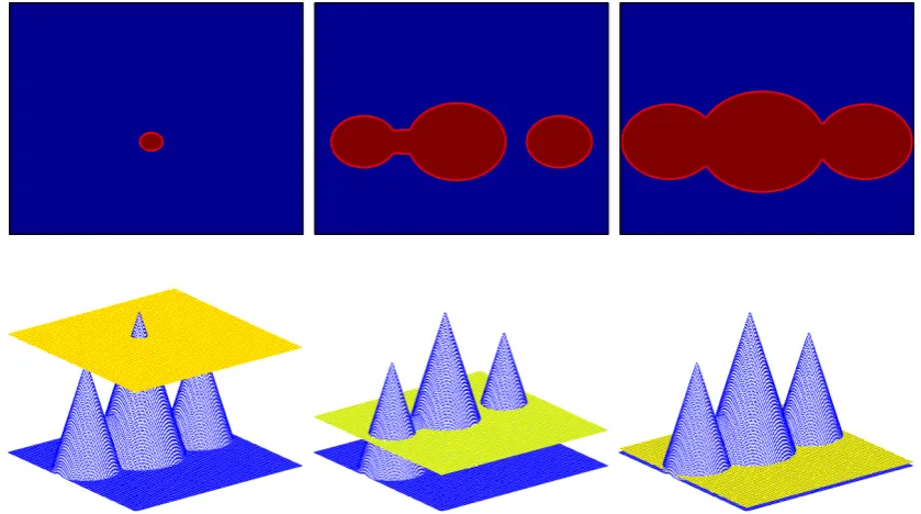
2.8 Illustration of how the level set function deal with topological changes. . 34

2.9 Evolution of a circular curve inward and outward. . . 36

2.10 Smoothing of contours represented by the zero level set. . . 37

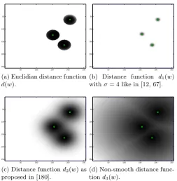
2.11 Comparison of several distance functions. . . 38

2.12 Gaussian kernel smoothed image. . . 46

2.13 Illustration of the enchantment using Laplacian. . . 46

2.14 Illustration of the 2-D enchantment using sharpening ﬁlters. . . 48

3.1 One dimensional signal restoration with TV model. . . 75

3.2 Approximation of the Heaviside and Delta function with Hϵ and δϵ. . . 86

4.1 Accurate approximation of second order RHAM obtained in 4 restarted iterations in comparison with the exact solution while HAM needs to be 8th order . . . 102

4.2 Comparison between RHAM obtained in 5 restarted iterations with HAM 10th order . . . 102

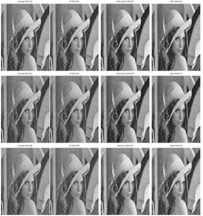
4.3 Comparison between TM and RHAM1 and RHAM2 for Lenna image with 10, 15 and 20 percent random noise . . . 113

(11)

4.5 Comparison between TM and RHAM1 and RHAM2 for geometric ﬁgures image with 10, 15 and 20 percent random noise . . . 115 4.6 Comparison between TM and RHAM1 and RHAM2 for rocket image

with 10, 15 and 20 percent random noise . . . 116 4.7 Comparison for segmentation between TM and RHAMs for geometric

ﬁgures image . . . 117 4.8 Comparison for segmentation between TM and RHAMs for CT image . 118 4.9 Comparison for segmentation between TM and RHAMs for UoL image . 118 4.10 Comparison for segmentation between TM and RHAMs for cameraman

image . . . 118 4.11 Comparison for segmentation between TM and RHAMs for MRI image 119 4.12 Comparison for segmentation between TM and RHAMs for galaxy image 119 4.13 Comparison for segmentation between TM and RHAMs for geometric

objects with circles image . . . 120 4.14 Segmentation of 3D geometric object and comparison between TM and

RHAMs . . . 121 4.15 Segmentation of diﬀerent 3D geometric object and comparison between

TM and RHAMs . . . 121 4.16 Test Set-3 Example 3. Successfully reached relative residual equal to

10−1 _{after 2 iterations for the RHAMs and 1000 iterations for TM. Due} to the size of the image TM CPU time was a few hours which is a great improvement with the RHAM which only required 5 minutes in this case. 122 4.17 Test Set-3 Example 4. Successfully reached relative residual equal to

10−1 by segmenting the vessels after 2 iterations for the RHAMs and for TM more than 100 iterations are needed. . . 122 4.18 Test Set-3 Example 5. Successfully reached relative residual equal to

10−1 by segmenting a CT image near the kidney after 2 iterations for the RHAMs and for TM more than 100 iterations are needed. . . 122 4.19 Test Set-3 Example 6. Successfully reached relative residual equal to

10−1 by segmenting a CT image near the spleen after 3 iterations for the RHAMs and for TM more than 100 iterations are needed. . . 123 5.1 Illustration of notation of selective segmentation models with n1 = 3

markers. . . 129 5.2 An image of a 2-D triangle over a rectangle with small intensity diﬀerence.129 5.3 Successful selective segmentation of two objects with similar intensities

by the dual level set selective segmentation model [129] and its compar-ison with old model of [12]. . . 130 5.4 Successful detection with dual level set method of the spiral in a clean

(12)

5.5 Successful detection with dual level set method of the right kidney in a real CT image with 3 markers. . . 143 5.6 Successful detection with dual level set method (a) of the ﬂower in a

clean and synthetic image with 3 markers; (b) cameraman in a clean and real image with 3 markers; (c) one cell in a real image with 3 markers.144 5.7 Successful detection with dual level set method of a) one coin in a strong

noise image with 3 markers; (b) one cell in a real image of mouse em-bryonic stem cells with 3 markers; (c) selection of the main galaxy with 3 markers. . . 145 5.8 Identical results by dual level set and Badshah-Chen [12] of the box with

4 markers. . . 146 5.9 Identical results by dual level set and Badshah-Chen [12] of the cross

with 4 markers. . . 147 5.10 Identical results by dual level set and Badshah-Chen [12] of the knee cap

with 4 markers. . . 147 5.11 Successful selective segmentation of the right kidney with 3 markers

with the dual level set model in comparison with unsuccessful result by Badshah-Chen [12] model. . . 148 5.12 Successful selective segmentation of a non-convex shape with 3 markers

with the dual level set model in comparison with unsuccessful result by Badshah-Chen [12] model. . . 148 5.13 Successful selective segmentation of a single cell with 3 markers with the

dual level set model in comparison with unsuccessful result by Badshah-Chen [12] model. . . 149 5.14 Successful selective segmentation of a cell with with 3 markers with the

dual level set model in comparison with unsuccessful result by Badshah-Chen [12] model. . . 149 5.15 Comparative results and importance of selective segmentation with

Chan-Vese [39] model. . . 150 6.1 Result of segmenting a 3D CT brain data set with Chan-Vese model in

the resolution of 64×64×64. . . 153 6.2 Result of segmenting a 3-D artiﬁcial geometrical image of resolution

128×128×128 with 4 spheres with Chan-Vese model. . . 153 6.3 Successful segmentation of a geometrical artiﬁcial object using the 3-D

Badshah-Chen and Gout-Guyader method. . . 159 6.4 Successful segmentation by the Badshah-Chen model [12] of a given

ge-ometric volume with two cuboid within a small gap in between. . . 159 6.5 Successful segmentation by the Gout-Guyader model [69] of a given

(13)

6.6 Failed segmentation by the Badshah-Chen model of a 3D object with two spheres. . . 161 6.7 Failed segmentation by the Gout-Guyader model [69] of a 3-D object

with two spheres in long term iterations. . . 162 6.8 A challenging test image for the Badshah-Chen and Gout-Guyader

mod-els. The given image consisted of a triangular prism over a cuboid and the two objects have a small intensity diﬀerence of 5 units. The models segment both the objects by failing to segment the aimed triangular prism.163 6.9 Contour-surface generated by a polytetrahedron. . . 169 6.10 Successful detection of the pyramid in a clean and synthetic 3D image

with 4 markers with 3-D dual level set method. . . 170 6.11 Successful detection of one sphere out of two in a clean and synthetic

3-D image with 4 markers with 3-D dual level set method. . . 170 6.12 Successful detection of the small cuboid in a clean and synthetic 3-D

image with 4 markers with 3-D dual level set method. . . 171 6.13 Successful detection of one sphere out of 4 in a clean and synthetic 3-D

image with 4 markers with 3-D dual level set method. . . 171 6.14 Successful detection of the prism in a clean and synthetic 3D image with

6 markers with 3-D dual level set method while the Badshah-Chen [12] fails. . . 172 6.15 Successful detection of the left kidney in a 3-D CT volume data with

3-D dual level set method. . . 173 6.16 Successful detection of the right kidney in a 3-D CT volume data with

3-D dual level set method. . . 174 6.17 Successful detection of liver in a 3-D CT volume data with 3-D dual level

set method, while the old models fail. . . 175 6.18 Slices in xy direction after segmentation of brain CT image with low

glioma with 3-D dual level set. . . 176 6.19 CT image post processed with Chan-Vese and Li-Kao-Gore-Ding model. 176 6.20 CT 3-D volume image post processed with Chan-Vese and

Li-Kao-Gore-Ding model. Blood ﬂow into veins has been distinguished. . . 177 6.21 3-D volume image post processed with Chan-Vese and Li-Kao-Gore-Ding

models. . . 178 7.1 Illustration of an inﬁnite perimeter function . . . 180 7.2 Successful segmentation with inﬁnite selective segmentation model of

the vase with markers set in the boundary of second tree (target object) using time marching algorithm . . . 187 7.3 Successful segmentation of diﬀerent images using inﬁnite selective

(14)

7.4 Successful segmentation for diﬀerent images with oscillatory boundaries with the AOS inﬁnite selective segmentation model. . . 189 7.5 Successful segmentation of two tips of leaves with oscillatory boundaries

with the AOS inﬁnite selective segmentation model. . . 190 7.6 Successful segmentation of one of the trees in an image with diﬀerent

trees with the AOS inﬁnite selective segmentation model. . . 191 7.7 Successful selective segmentation of palm trees and the respective

crop-ping with the AOS inﬁnite selective segmentation model. First column with old model using H1 Hausdorﬀ measurement second column new model with L2 measurement. . . 192 7.8 Successful selective segmentation of pine trees and the respective

crop-ping with the AOS inﬁnite selective segmentation model. First column with old model using H1 Hausdorﬀ measurement second column new model with L2 measurement. . . 193 7.9 Successful selective segmentation of pine branch and the respective

crop-ping with the AOS inﬁnite selective segmentation model. First column with old model usingH1 Hausdorﬀ measurement and the second column new model with L2 measurement. . . 194 8.1 Comparison between the new model and Badshah-Chen model [12] for

the case of two object with small intensity diﬀerence. . . 213 8.2 Comparison between the new model and Badshah-Chen model [12] for

CT and biological images. . . 214 8.3 Test Set 2 – Comparison with Nguyen-Cai-Zhang-Zheng model [8].

Suc-cessful result by Nguyen-Cai-Zhang-Zheng model for the case of kidney segmentation in a CT image. . . 215 8.4 Test Set 2 – Comparison with Nguyen-Cai-Zhang-Zheng model [8].

Suc-cessful result by new model for the case of two cells with same intensity and semi-transparent boundaries. . . 216 8.5 Test Set 2 – Unsuccessful result by Nguyen-Cai-Zhang-Zheng model [8]

(15)

List of Tables

4.1 Test Set-1: Gaussiannoise applied to the image. Required iterations for diﬀerent methods (with ∆t= 0.01) to achieve the PSNR values obtained from RHAM1 and RHAM2 by use of stopping criteria P SN R(un) <

P SN R(un−1). The Xapplies for cases when the TM method can have the same PSNR as RHAM, otherwise column four gives the maximum PSNR reached with the TM method. . . 124 4.2 Test Set-1: Gaussian noise applied to the image. CPU time for

dif-ferent methods (with ∆t= 0.01) to achieve the PSNR values obtained from RHAM1 and RHAM2 by use of stopping criteria P SN R(un) <

P SN R(un−1). The Xapplies for cases when the TM method can have the same PSNR as RHAM, otherwise column four gives the maximum PSNR reached with the TM method. . . 124 4.3 Test Set-1: Uniform random distributed noise. Required iterations for

diﬀerent methods (with ∆t= 0.01) to achieve the PSNR values obtained from RHAM1 and RHAM2 by use of stopping criterion P SN R(un) <

P SN R(un−1). . . 125 4.4 Test Set-1 Uniform random distributed noise. CPU time for diﬀerent

methods (with ∆t = 0.01) for to achieve the PSNR values obtained from RHAM1 and RHAM2 by use of stopping criterion P SN R(un) <

P SN R(un−1). . . 125 4.5 Test Set-1: AOS withGaussian noise applied to the image to be

com-pared with Tables 4.1-4.2. Required iterations for the AOS method (with ∆t= 0.01, 0.1 and 1) to achieve the PSNR values obtained from RHAM1 and RHAM2. The bold numbers in the PSNR columnsin table (4.5) shows that the PSNR of both AOS and the RHAMs have been the same, the rest of non bold PSNRs is the maximum that the AOS method could achieve. . . 126 4.6 Test Set-2: Comparison of RHAM with TM. Comparison for CPU time

(16)

4.7 Test Set-2: Comparison of RHAM with AOS. CPU time recorded for the iteration needed to have a given residual as shown in the respective picture. . . 127 4.8 Test Set-2: Comparison of RHAM with AOS. Maximum iterations needed

to have a given residual as shown in the respective picture. . . 127 4.9 Test Set-2: Comparison of RHAM with TM. Comparison for CPU time

recorded and the maximum iteration needed to have a given residual as shown in the respective pictures between the Time Marching, RHAM1 and RHAM2 methods. . . 127 8.1 Required CPU time for successful selective segmentation for some of the

(17)

Chapter 1

Introduction

1.1 Image Processing and Variational Modeling

Nowadays computer vision, especially image processing, plays an increasingly important role in diverse subjects such as medical imaging, geophysics, geodesy, atmospheric science, medicine, biology, engineering, photography, film and video production, remote sensing, security monitoring etc. After modern photography was invented during the 18-th century by Louis-Jacques-Mandé Daguerre, which improved the process already established by Joseph-Nicéphore Niépce, the invention of charge-coupled device (CCD) opened the path for digital photography development and allowed not only storage but also computer processing for the images. In 1895, X-ray was invented,1 and in the 1970s X-ray computed tomography (CT) becomes an important tool in medical imaging. A CT scanner uses ionizing radiation (X-ray) to obtain the image data. In 1977, another type of image, which was based on the emission and absorption of electro-magnetic energy in the radio frequency (RF) range of the electrostatic spectrum was introduced by Paul Lauterbur and Peter Mansfield, is called the magnetic resonance imaging (MRI) scanner. These and other imaging tools are becoming more and more important in the modern world as a source of diagnosing illnesses, catching criminals, postmortal identification, etc.

Digital images are proper 2-dimensional (2-D) projections representations of the visual world surrounding us containing various objects. A 2-D digital image can be presented as a 2-dimensional array of data z(x, y), where (x, y) represent the pixel location 2. The pixel value corresponds to the brightness of the image at location (x, y). Some of the most frequently used image types are binary, gray-scale and color images. Binary images has only two possible values for each pixel, black and white, where black is represented with the value 0 while white with 1. They are also referred to as 1 bit/pixel images. Gray-scale images, also called monochromatic, represents the brightness of the image by carrying only intensity information. Gray-scale images contains 8 bits/pixel data, which means 256 diﬀerent intensities (i.e., shades of gray) to

1_{http://inventors.about.com/library/inventors/blxray.htm} 2

(18)

50 100 150 200 250 50 100 150 200 250

50 100 150 200 250 50

100

150

200

250

50 100 150 200 250 300 50 100 150 200 250 300

10 20 30 40 50 60 70 80 90 100 110 10 20 30 40 50 60 70

50 100 150 200 250 300 350 400 450 500 50 100 150 200 250 300 350 400 450 500

10 20 30 40 50 60 70 80 90 10 20 30 40 50 60 70 80 90

10 20 30 40 50 60 70 80 10 20 30 40 50 60 70 80

50 100 150 200 250 300 350 400 450 500 50 100 150 200 250 300 350 400 450 500

[image:18.595.121.526.69.405.2]

100 200 300 400 500 600 100 200 300 400 500 600

Figure 1.1: Sample images used in our experiments. Images in top row are real life and artiﬁcial images, the images in second row are MRI and CT images taken in hospital environments and images in third row are biological images of cells. The last image in this row is a color image.

be recorded between 0 (representing black) and 255 (representing white). Color images are considered as three-channel monochrome images, where one channel of information is dominated by red, another by green and the third by blue. The color image is produced by mixing together various proportions of red, green and blue lights. This is a 24 bits/pixel image and it is referred to as an RGB image. In discrete sense a grey image is a 2-D array of numbers (matrix) while a color image is a 2-D array of vectors (composed by three chancels). In continuous sense a grey image is a 2-D function

z(x, y) and color image is a 2-D vector function (r(x, y), g(x, y), b(x, y)). In this thesis we mainly work on grey value images. Fig. 1.1 shows some examples of images which will be used for our experimental work in coming chapters.

(19)

programming. Therefore we have to develop mathematical models, algorithms and technologies with vision capabilities as advanced as human eyesight at least. Due to the wide specific application there is currently no single image processing method that yields acceptable results for every image and problem and for more some of the existing methods can at best deal with specific images only. Some of the techniques have been around already for some time and deeply investigated, though there is still room for improvement, others are relatively new and many challenges are still open for research. The field that includes methods for processing, analyzing, acquiring, and under-standing images from the real world in order to produce numerical or symbolic infor-mation is called Computer Vision. Computer vision is divided into image processing, pattern recognition, motion analysis, statistical learning etc., which employs a range of more or less well-defined measurement problems or processing problems that can be solved using a variety of methods. The objectives are as varied as

• registration, mapping, comparing and combining two diﬀerent views of the same object of a reference image into a target image,

• restoration and removal of noise (sensor noise, motion blur, etc.) from images,

• detection and recognition of objects in images,

• segmenting and picking out a feature of interest in an image from the rest of the image (the background),

• following the movements of a smaller set of interest points or objects in the image sequence (tracking of objects in videos),

and so on. In this thesis we look into a speciﬁc branch of image processing calledImage Denoising and mainly into Image Segmentation which is a challenge and has various research open problems.

Due to the corruption of the real signals by noise (unwanted signals) in an image, during acquisition, transmission, and retrieval from storage media, images require pre-processing which removes the noise and restores the image as close as possible to the original image. Fig. 1.2 is an example of such an image which shows the photography of a boat taken with a digital camera.

(20)

(a) Clean Boat Image, z(x,y) (b) Noise, n(x,y) (c) Noisy Boat Image, u(x,y)

Figure 1.2: Illustration of noise in the boat image.

white Gaussian noise. The performance of each algorithm is compared by computing PSNR (the peak signal to noise ratio) or SNR (signal to noise ratio) besides the visual interpretation. Those measures are deﬁned in Section§4.5.

The denoising problem can be mathematically presented as follows,

z(x, y) =u(x, y) +n(x, y) (1.1) where z(x, y) is the observed noisy image, u(x, y) the original image and n(x, y) the noise with varianceσ. The objective is to estimatez(x, y) given u(x, y).

Image segmentation is about partitioning an image into multiple segments (sets of pixels) and disjoint sub-regions by modelling the similarity characteristic and common features of the desired object while dealing with variation in intensity, scale, pose, and shape. Image segmentation is typically used to locate objects and boundaries (lines, curves, etc.) in images, to simplify and/or to change the representation of an image into something that is more meaningful. No single image segmentation technique performs well for all kinds of images, and problems; and in addition, the performance of various segmentation techniques is not the same and may vary from image to image. Segmentation should stop when the region of interest has been isolated. Due to this property the segmentation problem depends on the kind of the problem. In our work we have been dealing with the following problems for image segmentation:

• Develop a fast segmentation algorithm in order to extract the desired objects from the image background.

• Develop an automated selective/interactive segmentation method which has as an outcome a target object separated from other objects in the image.

Figure 1.3 shows two diﬀerent segmentation problems where the ﬁrst image is an ex-ample of image segmentation in which the boundaries of the objects are required to be segmented, shown as the contours of all letters in the the UoL image, and in the second image only the contour of the right kidney is the target object in a CT image.

(21)

(a) UoL Image Segmentation

20 40 60 80 100 120

20

40

60

80

100

120

(b) Right Kidney Image Selective Seg-mentation

Figure 1.3: Illustration of segmentation of the UoL image and selective segmentation of a CT image where the right kidney is the object of interest.

until a steady state is reached, thereby we separate the objects from background or separate an object from other objects. The evaluation of the quality of segmentation outcomes is typically based on the visual inspection of the images and is critical to measure the eﬃciency of segmentation algorithms. The evaluation of the outcome of segmentation algorithms is made with human interaction.

For both the branches mentioned above as well as for image processing tasks in general, variational techniques are promising models to solve those problems. Finding the solution of variational models implies minimization of nonlinear functionals leading to numerical solution of Euler-Lagrange equations which are nonlinear partial differen-tial equations (PDEs). Because of the discrete nature of the images, after using finite differences these PDEs are discretized and the models benefit from well-founded mathe-matical theories that allow us to analyze, understand and improve the existing methods. The Euler-Lagrange equation of these models is often described using parabolic PDEs, which are iterated in time until it reaches a steady state.

(22)

denoising problem the restarted homotopy analysis method is applied to the Rudin-Osher-Fatemi denoising total variation equation [136, 135], which is a successful tool for image restoration and for Chan-Vese Active Contour Without Edges model [37] for image segmentation. The Chan-Vese model [37], which seeks the desired segmentation as the best piecewise constant approximation to a given image, is the most popular method in image segmentation. This method represents the contour with a zero level-set function originally developed by Osher and Sethian [122]. The basic idea is to start with initial boundary shapes, which in general are represented in the form of circular or rectangular closed curves, and iteratively modify them by applying shrink/expansion operations according to the constraints of the image. For both of these models, and similarly with other imaging processing models, the Euler-Lagrange equations associ-ated are nonlinear PDEs. The restarted homotopy model will be compared with fast solvers such as the additive operator splitting method [174].

In the second part of the thesis we focus on variational image selective segmentation and introduce novel selective segmentation methods using the variational framework of active contours. More recently, Gout-Guyader [66, 69] and Badshah-Chen [12] proposed two different variational models for selective segmentation. The Badshah-Chen model improved the Gout-Guyader model, which is based on the edge information of the object, with a term which gives information to the minimization function of the region of segmentation. Both models can segment a range of images, but there are cases which appear too challenging for either model. For this reason we first develop a novel selective segmentation level-set method that uses a dual level set variational formulation. The model uses two level sets, from which one level set function (global) selects and finds all the objects, and with another level set (local) which is the closest to the geometric constraints (markers). It is a combination of edge detection, markers distance function and active contour without edges. Experimental results show that our model is more robust than previous work. To improve the efficiency of this model in the case of oscillatory boundaries a new regularization term has been proposed. The replacement of the regularizing term which measures the length of feature’s boundaries with a H1 Hausdorff measure with L2 Lebesgue measure of theγ-neighborhood of the boundaries demonstrates the effectiveness of the proposed method for real life images with oscillatory boundaries. Even though the dual level set method is accurate the feedback of this method is a slow convergence in cases of large images or a 3-D process. For this reason we improve the one level set selective segmentation variational models by incorporating new terms of an adaptive parameter edge detection function and a new area-based fitting term which enhances the model’s reliability.

1.2 Image Denoising and Image Segmentation

(23)

etc., methods of refining, acquiring, editing and visualizing image data are under a fascinating and ongoing improvement. Several applications of image processing such as in astronomy, astro-physics, biology, chemistry, art, genetics, physics, and other areas, bring a host of problems in imaging. The first and the most common one is the influ-ence of noise which brings an inhomogeneous appearance of the surfaces or objects in an image. This is due to the limitation of the technology and low light illumination. Such problems can be easily faced in CT images, SAR images, smart camera images, etc. Although, the process of restoring the image has been widely investigated, there remain problems to be considered and better improvements are challenging.

A great challenge nowadays is to tackle automatically and identify intelligently ob-jects in an image, in applications such as Closed-Circuit Television (CCTV) monitoring of a subject or medical geometry of a particular organ or tumors, where the selection of one feature/object among many ones is required. This is an important task which, particulary in the medical environment, will open the window to substantially improv-ing patient diagnosis, treatment monitorimprov-ing, and pre-operative plannimprov-ing. This will not only help us to view any organ on its own or as a collection within the anatomy, im-proving the diagnosis as well as surgical planning for patients, but could also allow the analysis of the shape and size of a tumor prior to surgery, or monitor the progress of a patient by comparing the segmented tumor through various stages of treatment. This will eliminate the manual segmentation which is a daunting task, since partial body scans range from tens to hundreds to even thousands of slices.

Due to the complexity of the images, especially the irregular shapes and sizes of objects/organs in medical images, the segregation process can be a diﬃcult task. The edges can be diﬃcult to delineate from the other organs due to noise during the im-age data acquisition process, or due to similar density with the other surrounding objects/organs.

There is a need for an automated process where some form of a priori information about the object such as markers are provided by the user. Chapters 5 and 6 provide a discussion on the novel 2-D and 3-D various models for image selective segmentation techniques currently available. These models are generally designed and are not com-plicated for any non-professional person to use and for more there is no need of manual manipulation control.

1.3 Chapters of this Thesis

The rest of this thesis is organized as follows: Chapter 2

(24)

linear spaces, variations of a functional, bounded space of variations, ill-posed inverse problems, regularization for image processing and the level set methods will be shortly introduced. A discussion on the discretisation of partial differential equations (PDEs) on regular domains using finite difference methods and the iterative solutions of linear and nonlinear equations. An overview of implicit and explicit methods as well an intro-duction to fast solver algorithms, such as additive operator splitting and the homotopy analysis method, will be presented.

Chapter 3

This chapter is an introduction to variational models for image restoration and recon-struction techniques. The total variation (TV) regularization functional and some of its mathematical analysis and properties are introduced. Here we cover the TV de-noising models based on the Mumford-Shah idea and in particular discuss the active contour without edges model of Chan-Vese. Some existing models used for solving the partial diﬀerential equation arising from Rudin-Osher-Fatemi (ROF) model and the minimization of the Chan-Vese model will be brieﬂy discussed as well.

Chapter 4

A numerical discrete restarted homotopy analysis algorithm for solving the nonlinear partial diﬀerential equation of the TV model with applications in both denoising and segmentation is developed. This algorithm overcomes the nonlinearity of the TV model and at the same time gives a fast numerical scheme and a better method in terms of accuracy. Finally, numerical evidence will show the validity of the restarted discrete homotopy analysis method and that the method is eﬃcient and robust even for images with large ratios of noise. The work has been generalised for 3-D as well and is shown by experiments to have great speed for 3-D segmentation. Moreover we will show that the method can be easily extended to other nonlinear TV models.

Chapter 5

(25)

Chapter 6

This chapter is a generalisation of the two dimensional dual level set selective model presented already in Chapter 5. The dual level set model developed in this chapter is capable of automatically capturing a local object of some target region in three dimen-sional domain. An additive operator splitting method is developed for accelerating the solution process. Numerical tests show that the proposed model is robust in locally segmenting complex image structures.

Chapter 7

This chapter improves the dual level set model, which is detailed in the previous two chapters, for irregular and oscillatory object boundaries in a selective model. The min-imization energy replaces the Hausdorﬀ measure of the length of a feature’s boundaries (i.e. H1) with the Lebesgue measure of theγ-neighbourhood of the boundaries (i.e. L2 ). Experimental results show that in cases of real life images with oscillatory boundaries we get qualitative results demonstrating the eﬀectiveness of the proposed method for these cases.

Chapter 8

In this chapter we propose a variational single level-set selective segmentation based model which is much faster to implement than the dual selective segmentation model in Chapter 5. The model combines several new ideas including a new area-based fit-ting term, a new region-based fitfit-ting term and an adaptive parameter edge detection function. The new model will be compared to the dual level set selective segmentation model and will be shown to have the same efficiency and reliability. We also provide an answer to the existence and uniqueness of the solution associated to our problem as well using viscosity theory. Test results show that the model finds the desired target object successfully in various challenging cases and that it is not heavily dependent on the prior information of markers or the distance function in contrast with existing selective models.

Chapter 9

(26)

Chapter 2

Mathematical Preliminaries

This chapter covers some basic mathematical tools which will be used throughout the rest of the chapters of the thesis, helpful while reading and understanding them. Useful preliminary definitions, theorems and examples from normed linear spaces, variations of a functional, bounded space of variations, ill-posed inverse problems and regularization to image representation, the level set method and other commonly met methods in either linear algebra or advanced calculus literature will be introduced. A discussion of the discretization of partial differential equations (PDEs) on regular domains using finite difference methods and the iterative solutions of linear and nonlinear equations will be described.

We start by introducing the Vector Space, a basic mathematical structure formed by a collection of elements

u= (u1, . . . , un), v = (v1, . . . , vn). (2.1)

called vectors, followed by the deﬁnitions of the norm and of Normed Linear Spaces. Literature can commonly be found in either linear algebra or advanced calculus litera-ture such as [145, 88].

2.1 Normed Linear Spaces

Definition 2.1.1 (Linear Vector Space). Let F be a scalar field (usually of real or complex numbers) and V a vector set on which two operations, addition and scalar multiplication, have been defined. For u,v ∈ V, the sum of u and v is denoted by u+v, and if c is a scalar, the scalar multiple of u by c is denoted by cu. If the following axioms hold for all u,v,w∈V and for all scalars c, d∈F, then V is called a vector space and its elements are called vectors.

10 Axioms of a Vector Space:

1. If u,v ∈V,thenu+v∈V (closure under addition)

2. If u,v ∈V,thenu+v=v+u (commutativity under addition)

(27)

4. There exists an element0∈V , called a zero vector, such thatu+0=u for all u∈V (identity element of addition)

5. For each u∈V, there is an element −u∈V such that u+ (−u) =0 (existence of additive inverse)

6. If c∈F,and u∈V,thencu∈V (closure under scalar multiplication) 7. If u,v ∈V,and c∈F thenc(u+v) =cu+cv (distributivity)

8. If u∈V,and c, d∈Fthen (c+d)u=cu+du (distributivity)

9. If u∈V and c, d∈F thenc(du) = (cd)u (associativity of scalar multiplication) 10. There exists an element1∈V, called the multiplicative identity, such that1u=u

for allv ∈V(identity of scalar multiplication)

Definition 2.1.2 (Norm). For a given a vector spaceV over a subfield F⊆C, a real valued function N :V−→Ris called a norm on V if for all a∈F and all u,v∈V, it satisfies

1. N(v)>0 for all v= 0̸ ∈V and N(v) = 0 for v= 0, (separates points). 2. N(αv) =|α|N(v) for all α∈R and v∈V, (triangle inequality).

3. N(v+u)≤N(v) +N(u) for allv,u∈V, (positive homogeneity). A normis aseminorm if the 1-st property (separating points) is removed. A norm on a vector space Vinduces a metric on V by

d(v,u) :=N(v−u).

This metric is invariant under translations and homogeneity, i.e.

d(v+w,u+w) =d(v,u), d(λv, λu) =|λ|d(v,u).

The norm of a vectorxon the set of real numbers Ris usually represented by ∥x∥(or for simplicity in some cases |x|), and the function is denoted ∥ · ∥(or | · |).

Example 2.1.3 Some examples of norms

• The absolute value is a norm on the set of real numbersR.

• Euclidean norm of a vector:

Let x= (x1, x2, . . . , xn)∈Rn then

∥x∥=

√

x2

1+x22+. . .+x2n.

This gives the ordinary distance from the origin to the point x. Note that this norm can sometimes be written as ∥x∥2 or |x|.

• Infinity norm:

(28)

• p-norm of a vector:

Considerx∈Rn_{, then for any real number} _p_≥₁ _the _p_{-norm of} _x _{is deﬁned as}

∥x∥p =

( _n ∑

i=1

|xi|p

)1/p

, (2.2)

For p = 1 this norm is called the 1-norm and clearly, for p = 2 this is the Euclidean norm, and as p approaches∞the p-norm approaches the inﬁnity norm.

• Lp-norm of a function:

Consider a continuous functionf deﬁned on a domainΩsuch that∫_Ω|f(x)|p dx <

∞ with1≤p≤ ∞. Then

∥f(x)∥Lp =

(∫

Ω

|f(x)|p dx

)1/p

(2.3) deﬁnes the Lp-norm of f onΩ. This is a generalization of the previous example since now f is allowed to have arbitrarily many components.

The special case when p=∞ is deﬁned as

∥f(x)∥_∞= sup

x |

f(x)|. (2.4)

• Total Variation (TV) normof u: Ω⊆R2→R is deﬁned as

T V(u) = ∫

Ω

|∇u|dxdy.

and will be discussed in more detail later in this chapter.

Deﬁnition 2.1.4 (Normed Linear Space ). A vector space equipped with a norm (seminorm)∥.∥deﬁned on it is called a normed linear space (seminormed linear space).

This also means that a linear vector space together with an inner product deﬁned on it, is a special type of normed space.

Theorem 2.1.5 For p ∈ [1,∞], the space equipped with the Lp _{norm is a normed}

vector space.

Proof The proof of this theorem uses the content of Minkowski’s inequality, Theorem 2.1.19, shown below.

Deﬁnition 2.1.6 The space of all n-tuples of real numbers, (x1, x2, ..., xn) commonly

denoted x∈Rn, equipped with the Euclidean metric

d(x,y) = ( _n

∑

i=1

(xi−yi)

)1/2

(29)

Deﬁnition 2.1.7 (Cauchy Sequence). A Cauchy sequence in a normed vector space V is a sequence {xi}∞i=1 having the property that for any ε >0, there exists an N ∈N such that

∥xi−xj∥< ε, ∀i, j≥N.

Note that Cauchy sequence is a sequence where all the terms, except a counted number, become arbitrarily close to one another

Deﬁnition 2.1.8 (Banach Space). A normed spaceV is said to be a Banach space if every Cauchy sequence {xi}∞i=1 ⊂ V converges to an element x ∈ V (which means thatlimi→∞xi=x).

Deﬁnition 2.1.9 (Hibert Space). A Hibert space is a spaceVwith an inner product

⟨u, v⟩ such that every Cauchy sequence converges to an element of the spaceV.

A Hilbert space is always a Banach space, but the converse need not hold.

Deﬁnition 2.1.10 (Convex Set). A set S in a vector space V is said to be convex if, for allu, v∈S and all θ∈[0,1], the point

(1−θ)u+θv

is inS. In other words, every point on the line segment connecting u and v is in S . Deﬁnition 2.1.11 (Convex Functions). A functionf :S→R deﬁned on an convex setS of some vector space is called convex if

f(θu+ (1−θ)v)≤θf(x) + (1−θ)f(y) (2.5) for all x, y ∈ S and θ ∈ (0,1). If the inequality is always strict for u ̸= v, f is called strictly convex.

Example 2.1.12 Examples onR and Rn

• exponential: eax, for anya∈R on domain Ris convex.

• powers: xα _on _R+_{, for} _α_≥₁_{or α}_≤₀ _{is convex.}

• powers of absolute value: |x|p _on_R_,_for _p_≥₁ _{are convex.}

• aﬃne function: f(x) =aT_x₊_b _where _a_∈_Rn_{, x, b}_∈_Rn×1 _{is convex.}

• The norms: ∥x∥p =

( ∑n

i=1|xi|p

)1

p

, f or p ≥1; ∥x∥_∞ = maxk(|xk|) are

con-vex.

• The TV norm deﬁnite as in 2.1.11 ofu: Ω⊆R2→R

T V(u) = ∫

Ω

|∇u|dxdy

is a convex functional.

(30)

Deﬁnition 2.1.14 If A ∈V thenC(A) =V\A denotes the complement of the set A

in V, that is, the set of all points x∈A which do not belong to A.

Deﬁnition 2.1.15 (Closed Set). A subset A ∈ V is closed if its complement C(A) is open.

Deﬁnition 2.1.16 (Lipschitz Condition). If for any points x, y∈S ⊂R for some

M ∈R the real function f :S →Rsatisﬁes

|f(x)−f(y)| ≤M|x−y|

thenf is said to satisfy the Lipschitz condition inS and is called a Lipschitz continuous function.

Theorem 2.1.17 (Young’s Inequality for Products). If a andb are nonnegative real numbers and p and q are positive real numbers such that 1_q +1_p = 1, then

ab≤ a

p

p + bq

q .

Equality holds if and only if ap=bq.

Theorem 2.1.18 (H¨older’s Inequality). LetΩ∈Rnbe a domain andf ∈Lp(Ω), g∈ Lq(Ω) with 1 ≤ p, q ≤ ∞ such that 1_q + 1_p = 1. Then f g ∈ L1(Ω) and ∥f g∥L1_(Ω) ≤

∥f∥Lp_(Ω)∥g∥_Lq_(Ω).

Theorem 2.1.19 (Minkowski’s Inequality). Let Ωbe a normed space and1≤p≤

∞ and f, g∈Lp(Ω). Then f +g∈Lp(Ω)and

∥f+g∥_Lp_(Ω) ≤ ∥f∥_Lp_(Ω)+∥g∥_Lp_(Ω).

The Minkowski inequality establishes that for the Lp spaces the triangle inequality is satisﬁed and that the set ofpth power integrable functions, together with the function

∥ · ∥Lp, is a normed vector space.

2.2 Curves, Surfaces and Some Calculus and Geometry

Elements

2.2.1 Curves and Surfaces in Euclidean Spaces

Considering the space R2, the lower-dimensional interface is a curve that separatesR2 into subdomains with nonzero areas. Generally speaking, a curve is an object similar to a line but which is not required to be straight. In this thesis we are limiting our interface curves to those that are closed inR2 or a subdomain Ω⊆R2, and we denote the interface by∂Ω. In other words the curves we consider have clearly deﬁned interior and exterior regions.

(31)

deﬁned by ∂Ω = {x : |x| ≤ 1}. We also deﬁne the interior region, which is a unit open disk Ω− = {x : |x|< 1}, and the exterior region Ω+ ₌ _{_x _: _|_x_|_> ₁_}_{. These} regions are depicted in Fig. 2.1.

[image:31.595.245.383.153.296.2]

Note that a line is a special case of curve, a curve with null curvature1.

Figure 2.1: Representation of the curvex2+y2= 1.

The curve described above is given in an analytical way. In general, one needs to parameterize the curve with a vector functionϕ= (x(t), y(t)), where the parametert

is given in an interval [ta, tb], such that the condition of being a closed curve implies,

x(ta) =x(tb). The parametric equation for the circle above would be

ϕ(t) = (cos(t),sin(t)) for 0≤t <2π.

In the case of three spatial dimensions the lower-dimensional interface is a surface that separates R3 into separate subdomains with nonzero volumes. A surfaces is a two-dimensional topological manifold whith clearly defined interior and exterior regions. Example 2.2.2 Forx= (x, y, z)∈R3 considerϕ(x) =x2+y2+z2−1. The interface is defined by ϕ(x) = 0, or alternatively, the boundary of the unit sphere is defined by

∂Ω = {x : |x| ≤ 1}. The interior region can be deﬁned as an open unit sphere Ω−={x : |x|<1}, and the exterior region Ω+₌_{_x _: _|_x_|_>₁_}_.

2.2.2 Gradient, Mean Curvature and Some Geometry Element

Here we will give some deﬁnitions of geometric characteristics of the interface, starting with the deﬁnition of the gradient.

Deﬁnition 2.2.3 For a given scalar function ϕ(x1, x1, ..., xn) the gradient is denoted

as ∇ϕ or grad ϕ and is deﬁned as

∇ϕ=

(

∂ϕ ∂x1

, ∂ϕ ∂x2

, ..., ∂ϕ ∂xn

)

.

(32)

The gradient∇ϕis perpendicular to the isocontours ofϕand points in the direction of increasing ϕ. The unit (outward) normal vector n is a vector that points in the same direction as the gradient∇ϕfor points on the interface, and is deﬁned as

n= ∇ϕ

|∇ϕ|.

Deﬁnition 2.2.4 The mean curvature, or simply curvature, of the interface is deﬁned as the divergence of the unit normal n

κ=∇ · n=∇ · ∇ϕ

|∇ϕ| =

∂ ∂x1

(

∇ϕ

|∇ϕ|

) + ∂

∂x2 (

∇ϕ

|∇ϕ|

)

+...+ ∂

∂xn

(

∇ϕ

|∇ϕ|

)

(2.6) It can be shown that κ > 0 for convex regions, κ <0 for concave regions, and κ = 0 for a plane; shown in Fig. 2.2. In two dimensional space the curvature is equal to

κ= ϕ 2

xϕyy−2ϕxϕyϕxy +ϕ2yϕxx

(ϕ2

x+ϕ2y)3/2

,

and in three dimensional space

κ= ϕ 2

xϕyy−2ϕxϕyϕxy+ϕy2ϕxx+ϕ2xϕzz−2ϕxϕzϕxz+ϕ2zϕxx+ϕ2yϕzz−2ϕyϕzϕyz+ϕ2zϕyy

[image:32.595.114.542.162.563.2]

|∇ϕ|3 .

Figure 2.2: Representation of the curvature with convex regions κ > 0, and concave regionsκ <0.

2.2.3 Heaviside and Dirac Delta Functions

(33)

as follows:

Deﬁnition 2.2.5 The Heaviside function, usually denoted by H, is a non-continuous function whose value is zero for negative arguments and one for positive argument. For a given function ϕ(x), x∈Rn _{the Heaviside function is written:}

H(ϕ) = {

1 if ϕ≥0 0 if ϕ <0

Note that the characteristic function of the interior and exterior regions, denoted by

χ+ andχ− respectively, can be expressed in terms of the Heaviside function as follows

χ− =H(ϕ) andχ+= 1−H(ϕ) for all x.

Deﬁnition 2.2.6 For a given functionϕ(x), x∈Rn,the directional derivative of the Heaviside function H in the normal direction n is called Dirac delta function and is equal to

b

δ(x) =H(ϕ(x))′ · n=H′(ϕ(x))∇(ϕ(x))· ∇ϕ(x)

|∇ϕ(x)| =H

′₍_ϕ_(x))_|∇_ϕ_(x)_| _(2.7)

In one dimensional space, the delta function is deﬁned as the derivative of the Heaviside function,δ(ϕ) =H′(ϕ). The delta functionδ(ϕ) is identically zero everywhere except at ϕ= 0. This allows us to use 1-dimensional Dirac delta functions to rewrite then-dimensional Dirac delta function given by equation (2.7) as

b

δ(x) =δ(ϕ(x))|∇ϕ(x)|. (2.8) For a given functionf(x) deﬁned on Ω, the volume integral inside the boundary Γ =∂Ω is the integral of f(x) over the exterior regionχ−

∫

Ω

f(x)H(ϕ)dx.

In similar way, _∫ Ω

f(x)(1−H(ϕ))dx

representing the integral off(x) over the interior region χ+_{. The surface integral of a} functionf(x) over a boundary Γ is deﬁned as

∫

Ω

f(x)|∇H(ϕ)|dx= ∫

Ω

f(x)δ(ϕ)|∇ϕ|dx.

Note that if f(x) = 1, then this yields the surface area or volume of ∂Ω. In this way, for example inR2 , the area formula above can be rewritten

∫

R2

(34)

and the length of the interface Γ is ∫

R2|∇

H(ϕ)|dxdy= ∫

R2

δ(ϕ)|∇ϕ|dxdy.

2.3 Calculus of Variation

Calculus of variations seeks to ﬁnd the optimal shape, curve, surface, or processes when the optimality criterion is given in form of the integral of an unknown function. Math-ematically, this involves ﬁnding an appropriate function that makes a given quantity (usually an energy or integral) stationary which, in physical problems, is usually a min-imum or maxmin-imum. Because a function is varied, these problems are called variational and solved by the so-called calculus of variations. Calculus of variations highlights the interactions between analysts, geometers, and physicists and its reach in application problems which are fundamental in many areas of mathematics, physics, engineering and other applications. A good impression of this diversity can be obtained by reading the book entitled “The Parsimonious Universe”[74].

In this section we introduce the basic tools to compute the ﬁrst variation (also known as the Euler-Lagrange equation) of a functional. Extensive literature in this respect can be found in the monographies [58, 60, 61, 138, 128] or elsewhere.

2.3.1 Variation of a Functional

A functional is a function of another function (such as a curve, or a surface, etc.) which assigns a real number to each function in some class. The first variation of a functional deals with the problem of finding a function for which the value of a certain integral is either the largest or the smallest possible and the integrands of which are functions of independent variables, dependent variables, and the derivatives of one or more dependent variables. Classical solutions to minimization problems in the calculus of variations are prescribed by boundary value problems involving certain types of differential equations, known as Euler–Lagrange equations.

Consider the general functional J(u) : Ω→R J(u) =

∫

Ω

F(x, u(x),∇u(x))dx, (2.9) where Ω denotes some normed linear space (for example, Ω=Rn,n≥1) which is a solu-tion space of the funcsolu-tionu,∇u(x) denotes its gradient∇u(x) = (u(x)x1, u(x)x2, . . . , u(x)xn).

Heredx is the n-diﬀerential element deﬁned asdx=dx1dx2· · ·dxn.

Example 2.3.1 Simple examples of variational integrals (2.9) are the Dirichlet integral

D(u) = 1 2

∫

Ω

(35)

and the nonparametric arc length integral

L(u) = ∫

Ω √

1 +|∇u(x)|2_dx_. _(2.11) The minimisation problem, in other words the ﬁrst variation, consists of solving the following minimization problem:

min

u J(u). (2.12)

The most importantnecessarycondition to be satisﬁed by any minimizer of a variational integralJ(u) is the vanishing of its ﬁrst variation δJ(u)

δJ(u) = d

dεJ(u+εφ)

ε=0

= 0, (2.13)

where φ∈Ω is a test function and ε is a real parameter (which is restricted to some interval around 0). For someu0∈Ω, we callδJ(u0) the ﬁrst variation ofJatu0 in the direction of φ.

Example 2.3.2 A concrete example of both mathematical and practical importance would be the minimal curve problem of finding the shortest path between two specified locations. Given two distinct points(a, α)and(b, β)inR2the task is to find the curve of

Figure 2.3: The shortest path is a straight line.

shortest length connecting them. We know by intuition that the shortest route between two points is a straight line; see Fig.2.3, with equation of the form

y =cx+d= β−α

b−a(x−a)−α. (2.14)