Nonlinear instability and dynamics of polaritons in quantum systems

T h e o p e n – a c c e s s j o u r n a l f o r p h y s i c s

New Journal of Physics

Nonlinear instability and dynamics of polaritons in

quantum systems

P K Shukla1 and B Eliasson

Institut für Theoretische Physik, Ruhr-Universität Bochum, D-44780 Bochum, Germany

E-mail:[email protected]

New Journal of Physics9(2007) 98 Received 26 January 2007

Published 20 April 2007 Online athttp://www.njp.org/

doi:10.1088/1367-2630/9/4/098

Abstract. We present analytical and simulation studies of the nonlinear instability and dynamics of an electron–hole/anti-electron (hereafter referred to as polaritons) system, which are common in ultra-small devices (semiconductors and micromechanical systems) as well as in dense astrophysical environments and the next generation intense laser–matter interaction experiments. Starting with three coupled nonlinear equations (two Schrödinger equations for interacting polaritons at quantum scales and the Poisson equation determining the electrostatic interactions and the associated charge separation effect), we demonstrate novel modulational instabilities and nonlinear polaritonic structures. It is suggested that the latter can transport information at quantum scales in high-density, ultracold quantum systems.

Phenomena occurring at quantum scales are of paramount importance in diverse areas of physics, and have potential applications in ultra-small devices (e.g. semiconductors and micromechanical systems [1]–[3]), in dense astrophysical environments [4], in intense laser–matter interaction experiments [5], in quantum dots and nanowires [6], in biophotonics [7] and in cool vibes [8]. Quantum mechanical effects (e.g. tunnelling) become important when the de Broglie length is comparable to inter-particle distances in the quantum system. In such a situation, strong correlations among electrons or holes/anti-electrons (hereafter referred to as polaritons) in dense matter produce wavefunction dispersion at quantum scales. In dense quantum systems, the dynamics of polaritons is governed by the Wigner–Poisson (W–P) system that includes the dispersive effects. It turns out that the W–P equations can be represented in the form of generalized quantum hydrodynamic (GQH) equations, which somewhat resemble those describing the dynamics of Bose–Einstein condensates (BECs) in ultracold matter [9]. In quantum systems,

1 _{Author to whom any correspondence should be addressed.}

the polaritons obey Fermi–Dirac statistics and their dynamics is, in turn, governed by the nonlinear Schrödinger and Poisson equations. The latter are naturally deduced from the GQH equations within the framework of an eikonal representation [10].

Since the polaritons are building blocks of many physical systems as described above, it is timely to present some novel collective interactions involving nonlinear interactions among electrons and holes/anti-electrons in quantum mechanical systems. Specifically, in this paper we present analytical and simulation studies of nonlinearly interacting polaritons and demonstrate the possibility of a new class of modulational instabilities and localized nonlinear structures (bright and dark envelope excitations and quantum vortex pairs). The latter may be exploited to transport information at quantum scales in semiconductors and micromechanical systems.

Let us first present the mathematical model which governs the dynamics of a polariton system. The collective motion of the particles is in this model described by effective Schrödinger equations [10] for the electrons and holes/anti-electrons (denoted by the subscript ‘e’ and ‘h’, respectively), coupled with the Poisson equation,

i¯h∂ψe ∂t +

¯ h2 2me

∇2

ψe+eφψe −Weψe =0, (1)

i¯h∂ψh ∂t +

¯ h2 2mh

∇2_ψ

h−eφψh−Whψh =0, (2)

∇2

φ=4πe(|ψe|2− |ψh|2), (3)

where We =mev2Fe|ψe|4/D/2n 2/D

0 and Wh =mhv2Fh|ψh|4/D/2n 2/D

0 are the pressure terms due to the Fermi temperature of the electrons and holes/anti-electrons, respectively. Furthermore, vFe =(TFe/me)1/2andvFh=(TFh/mh)1/2are the Fermi speeds andTFe ∼h¯2n

2/3

0 /me andTFh ∼ ¯

h2n2₀/3/mhare the Fermi temperatures of the electrons and holes, andDis the number of spatial dimensions,me(mh) is the effective mass of the electron (hole), andn0is the equilibrium electron and hole number density. Hence, we have|ψe| = |ψh| =n

1/2

0 at equilibrium.

The system of equations (1)–(3) conserves the number of electrons and holes, Ne =

|ψe|2d3xandNh =

|ψh|2d3x, respectively, the total momentumP= −i¯h

(ψ∗_e∇ψe+ ψ_h∗∇ψh)d3x, the total angular momentum L= −i¯h

(ψ∗_er× ∇ψe+ψ∗_hr× ∇ψh)d3x, and the total energy E = [−h¯2ψ∗_e∇2_ψ

e/2me−h¯2ψ∗h∇2ψh/2mh+|∇φ|2/8π+D(We|ψe|2+ Wh|ψh|2)/(2 +D)] d3x. The total energy has been obtained from equations (1) and (2) by using the identity ∂∇φ/∂t =2πie¯h[(ψh∇ψ∗h−ψ∗h∇ψh)/mh−(ψe∇ψ∗e −ψ∗e∇ψe)/me], which is equivalent to the Poisson equation (3).

For the numerical analysis, it is convenient to introduce normalized variables so that a set of key parameters can be identified. Hence, normalizing the wavefunctions ψe and ψh by n1₀/2, the potential φ by TFe/e, the time t by the Fermi time tF=¯h/TFe, and the space

r by the Fermi radius λF =(TFe/4πn0e2)1/2, one obtains from (1)–(3) the normalized set of equations i∂ψe/∂t+Ae∇2ψe +φψe− |ψe|4/Dψe =0, i∂ψh/∂t+(me/mh)Ae∇2ψh−φψh− (me/mh)|ψh|4/D =0, and∇2φ = |ψe|2− |ψh|2, where we identify the parametersmh/meand the quantum coupling constantAe =2πe2me/¯h2n

1/3

We next consider the stability of the system (1)–(3). Using the Fourier decomposition

ψe =[ψe0+ψe+exp(iK·r−it)+ψe−exp(−iK·r+ it)] exp(iKe0·r−iωe0t), (4) ψh =[ψh0+ψh+exp(iK·r−it)+ψh−exp(−iK·r+ it)] exp(iKh0·r−iωh0t), (5) φ =φexp(iK·r−it)+φ∗exp(−iK·r+ it), (6) in (1)–(3), whereψe0andψh0are the envelopes of the equilibrium electron and hole wavefunctions and ψe±, ψh± (|ψe±|, |ψh±| |ψe0|, |ψh0|) and φ are the envelopes of the small-amplitude perturbations of the wavefunctions and potential, respectively, and sorting the equations by different Fourier components, we have the dispersion relations for the electron and hole zeroth order wavefunctions ¯hωe0−h¯2ke02 /2me−mev2Fe|ψe0|4/D/2n

2/D

0 =0 and ¯hωh0−h¯2k2h0/2mh− mhv2Fh|ψh0|4/D/2n

2/D

0 =0. We note from equation (3) that|ψe0| = |ψh0|(=n 1/2

0 ). The nonlinear dispersion relation for the small-amplitude density modulations is

(De+De−−γ_e2|ψe0|4)(Dh+Dh−−γ_h2|ψh0|4)−β2|ψe0|2|ψh0|2

×(De++De−+ 2γe|ψe0|2)(Dh++Dh−+ 2γh|ψh0|2)=0, (7) where we have denoted β=4πe2_/K2_{, γ}

e =β+ 2αe|ψe0|4/D−2/D, γh =β+ 2αh|ψh0|4/D−2/D, αe =mev2Fe/2n

2/D

0 andαh =mhv2Fh/2n 2/D

0 . Here the nonlinear wave modes are characterized by

De± = ±

¯ h+ h¯

2

me

Ke0·K

−¯h2K2 2me

−β|ψe0|2−

2αe|ψe0|4/D

D , (8)

Dh± = ±

¯ h+ ¯h

2

mh

Kh0·K

−h¯2K2 2mh

−β|ψh0|2−

2αh|ψh0|4/D

D . (9)

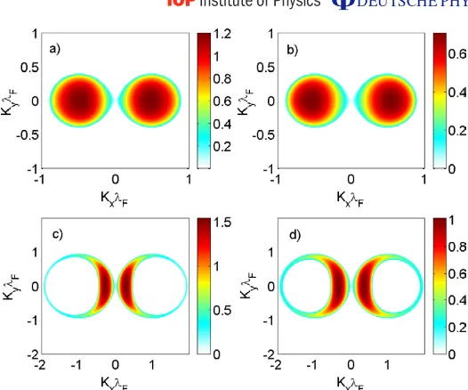
We have solved the dispersion relation (7) numerically and have presented the growth rate (the imaginary partγ of) in figure1. We have taken the coupling constantAe =5 and have assumed a two-dimensional (D =2) geometry in thex–y-plane. The used mass ratiomh/me =1 is typical for light holes while mh/me =5 is typical for heavy holes [11]. We have taken the wavevectors Ke0 and Kh0 with opposite signs and directed along the x-axis, Ke0 =xke0 and

Kh0 =xkh0, wherex is the unit vector in the x-direction. Hence, the electrons and holes are counter-streaming, and this gives rise to a streaming instability, as can be seen in figure 1. For the smaller wavenumber |ke0| = |kh0| = 0.5λ−F1, the growth rate is smaller than for the larger wavenumber |ke0| = |kh0| =1.0λ−F1. Comparing the panels (a) and (b) with panels (c) and (d) of figure1, we also see that the wave modes for the larger|ke0|and|kh0|have a wider spectrum of growing waves in oblique directions to the x-axis, while the wave modes for the smaller wavenumbers have growing wave modes primarily in thex-direction. Whenke0andkh0are taken to be equal to each other, then the system is stable, i.e. the dispersion relation (7) has only real-valued roots in this case. In order to study the nonlinear saturation of the streaming instability, we have solved the time-dependent system of equations (1)–(3) numerically, and have presented the results in figure2. As initial conditions we usedψe =n

1/2

0 exp(ike0x)andψh =n 1/2

Figure 1. The growth rateγ (in units oft_F−1) as a function of the wavenumbers Kx and Ky, for (a): mh/me =1, ke0 =0.5λ−F1 and kh0 = −0.5λ−F1, (b): mh/me =5, ke0 =0.5λ−F1 and kh0 = −0.5λ−F1, (c): mh/me =1, ke0 =1.0λ−F1 and kh0 = −1.0λF−1, and (d): mh/me =5, ke0 =1.0λ−F1 and kh0 = −1.0λ−F1. We usedAe =5 in all cases.

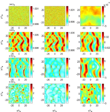
where we added a low amplitude noise (random numbers) of order 10−3_n1/2

0 to give a seed for any instability. We used the parameters in panel (d) of figure 1, i.e. the mass ratiomh/me =5 and wavenumberske0 =1.0λ−F1andkh0 = −1.0λ−F1. We see in figure2that density waves grow primarily in thex-direction, with a wavelength ofλ=12λF, corresponding to the wavenumber Kx≈0.5λ−F1 of the fastest growing wave in the upper right panel of figure 1. In the nonlinear stage, att =12tF, very narrow density humps are formed at which both the electrons and holes are accumulated. At the later staget =14tF, these density maxima break up into a chaotic pattern of very localized density patches. We see that the density maxima at all times are associated with a positive potential.

We next investigate the existence of two-dimensional (D=2) vortex structures in our electron–hole system. Assuming that the electron and hole wavefunctions are in the form ψe =e(r)exp(iMeθ−iet) and ψh =h(r)exp(iMhθ−iht), where e and h are real-valued functions, r and θ are the polar coordinates defined by x=rcosθ and y=rsinθ, e and h are constant frequency shifts andMe =0, ±1, ±2, . . .andMh =0, ±1, ±2, . . .are the different excited states (charge states) of the vortices, the system of equations (1)–(3) takes the form

¯ h2 2me

d2 dr2 +

1 r

d dr −

M_e2 r2

e+(¯he+eφ−We)e =0, (10)

¯ h2 2mh

d2 dr2 +

1 r

d dr −

M_h2 r2

Figure 2. The electron number density (left column), hole number density (middle column) and potential (right column) at times t=0tF, 6tF, 12rF and 14tF formh/me =5, ke0 =1.0λF−1, kh0 = −1.0λ−F1 andAe =5. The number densities are normalized byn0and the potentialφ byTFe/e.

d2 dr2 +

1 r

d dr

φ=4πe(|e|2− |h|2). (12)

For a localized structure, we have d/dr =0,φ =0,|e| = |h0| =n 1/2

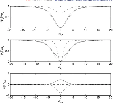
0 atr= ∞, and it follows that the frequency shifts take the forms e =mev2Fe/2¯h and h=mhv2Fh/2¯h. At r=0, we have the boundary conditions de/dr =dh/dr=dφ/dr=0, and it follows thate =0 when Me =0 andh =0 whenMh =0. The numerical solutions of the system (10)–(12) are presented in figure 3for a few sets of parameters. We see that the electron vortices withMx =1 show a

–200 –15 –10 –5 0 5 10 15 20 0.5

1

r/λ_F

|

Ψe

|

2 /n

0

–20 –15 –10 –5 0 5 10 15 20

0 0.5 1

r/λ_F

|

Ψh

|

2 /n

0

–20 –15 –10 –5 0 5 10 15 20

–1 0 1

r/λ_F

e

φ

/

TFe

Figure 3. The electron number density (upper panel), hole number density (middle panel) and the potential (lower panel) for a two-dimensional vortex with the charge statesMe =1 andMh =0 (solid lines),Me =0 andMh =1 (dashed lines) andMe =Mh =1 (dash-dotted lines). We used the parametersAe =5 and mh/me =5.

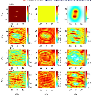
the system decouples completely into systems similar to those used to model BECs. In order to assess the dynamics and interaction between vortices, we have solved the time-dependent system (1)–(3) numerically, and as initial conditions we have used electron density perturbations in the form of vortex-like structures. The results are presented in figures4and5. In figure4, we used the initial condition ψe =n

1/2

0 f1f2f3f4, wherefj =tanh(

(x−xj)2+(y−yj)2)exp [+

Figure 4. The electron number density (left column), hole number density (middle column) and the potential (right column) for two interacting vortex pairs at times t =0tF, 12tF, 24tF and 30tF. We used the parameters Ae =5 andmh/me =5. The same normalization of variables as in figure2is used.

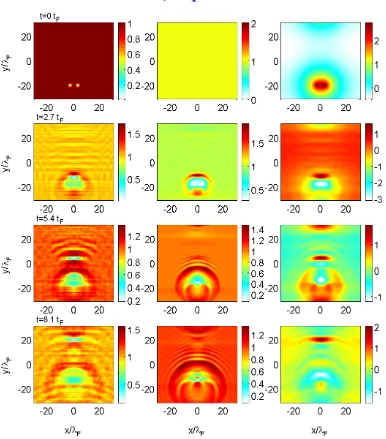
Figure 5. The electron number density (left column), hole number density (middle column) and the potential (right column) associated with a vortex pair at times t =0tF, 2.7tF, 5.4tF and 8.1tF. We used the parameters Ae =5 and mh/me =5. The same normalization of variables as in figure2is used.

References

[1] Markowich P Aet al1990Semiconductor Equations(Berlin: Springer) [2] Baranger H Uet al1993Chaos3665

[3] Berggren K-F and Ji Z-L 1996Chaos6543 [4] Opher Met al2001Phys. Plasmas82454

Marklund M and Shukla P K 2006Rev. Mod. Phys.78591 Chabrier Get al2002J. Phys.: Condens. Matter149133

[5] Becker K H, Schoenbach K H and Eden J G 2006J. Phys. D: Appl. Phys.39R55 [6] Shpatakovskaya G V 2006JETP—Sov. Phys.102466

[7] Barnes W Let al2003Nature424824 [8] Killian T C 2006Nature441297

[9] Kolomeisky E Bet al2000Phys. Rev. Lett.851146 [10] Manfredi G and Haas F 2001Phys. Rev.B64075316

Manfredi G 2005Fields Inst. Commun.46263