The role of primitive part modelling within an integrative simulation environment

THE ROLE OF PRIMITIVE PART MODELING WITHIN AN INTEGRATIVE

SIMULATION ENVIRONMENT

T.T. Chow

, J.A. Clarke

, and C.L. Song

1

Division of Building Science & Technology, City University of Hong Kong,

Hong Kong SAR, China

2

Energy Systems Research Unit, University of Strathclyde, Glasgow, Scotland, G1 1XJ

ABSTRACT

The component-based modeling approach to the simulation of HVAC systems has been in used for many years. The approach not only supports plant simulation but also allows the integration of the building and plant domains. Frequently, however, the plant models do not match exactly the types being used in a given project and where they do, may not be able to provide the required information. To address such limitations research has been undertaken into alternative approaches. The aim of such research is to provide a modeling approach that is widely applicable and offers efficient code management and data sharing. Primitive Part (PP) modeling is one such effort, which employs generic, process-based elements to attain modeling flexibility. Recent efforts have been on the development of data structure and graphics that facilitates PP auto-connection via computer interface. This paper describes the approach using an example application and its suggested role within an integrative simulation environment.

INTRODUCTION

Many contemporary building simulation programs utilize a component-based approach to plant simulation, e.g. TRNSYS (Solar Energy Laboratory 2000), ESP-r (ESRU, 2000) and ENERGY+ (Crawley et al., 2001). The range of component models contained within the libraries of such systems can support an extensive range of assessments for a large number of HVAC system types. The user will typically interconnect component models to form a network corresponding to the desirable topology. Thereafter, the simulation engine calls upon its component models, treating them either as an energy input/output model or as a model generatorthe so-called sequential and simultaneous solution approaches. Time step iteration is then used to solve tightly coupled problems. This modular approach allows users to undertake innovative analyses that transcend conventional HVAC design practice. Performance studies of solar thermal/photovoltaic systems, and other renewable energy systems, can be readily supported. Where a component model does not exactly match the equipment types selected for a

given project, users may have to develop a bespoke model that encapsulates relevant algorithms and physical parameters. This is a non-trivial task, demanding software engineering skills and time spent on validation work. This applicability problem has given impetus to a search for alternative modeling approaches that offer inherent configurability. Several such projects may be identified, including the SPARK system (Buhl et al., 1993), the Neutral Model Format (NMF) (Sahlin et al., 1995), the IDA system (Sahlin, 1993) and Primitive Part (PP) modeling (Chow et al., 1997). The PP modeling approach described here allows any component model to be built from a pre-formed set of generic, process-based elements.

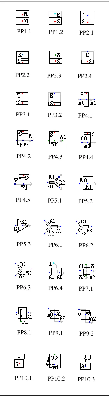
Essentially a PP model comprises a conservation equation-set relating to a small control volume and describes a specific thermo-fluid process [8]: plant equipment, and hence whole networks, can be modeled by simple PP combination. Each PPs exists as an individual subprogram. Figure 1 lists the 27 PPs that have been developed to support the modeling of contemporary HVAC systems. The expectation is that additional PPs will be added as and when new physical processes, as opposed to new component types, are encountered. An interface program exists to support the construction of component model sub-assemblies and their subsequent interconnection to define an envisaged HVAC layout. This interface program is contained within an integrated modeling system so that it is possible to rapidly increase the modeling detail as the design evolves. This allows the use of a detailed modeling approach throughout the design process, rather than using a progression of toolsfrom simplified to detailedand thereby ignoring the many theoretical discontinuities and contradicting assumptions.

INTEGRATIVE SIMULATION

ENVIRONMENT

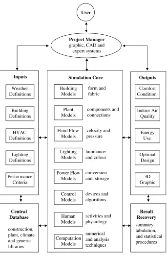
1999). In this way, the systemic, dynamic, non-linear and complexity characteristics of the building system may be addressed. Figure 2 shows the components of an integrative simulation environment. CAD tools may be used to create a building model of arbitrary complexity. This model may then be imported via a central 'Project Manager'. Its function is to co-ordinate problem definition and give/receive the data model to/from the simulation engine when the design hypothesis changes. On receipt of a system of equations defining a problem, the simulation engine invokes appropriate solvers to obtain the evolving state variables for post-processing against due considerations of human physiological responses, relevant design standards, performance goals and so on. A number of performance assessment tools are provided to assist with results analysis and the composition of 'integrated performance views' to communicate overall performance to other members of the design team and the client. Significantly, in the present context, the Project Manager provides access to databases to support the model attribution process. It is here that greater flexibility is required in relation to the selection and adaptation of plant component models.

In the conventional approach to component model formulation, different approaches may be adopted. These approaches include empirical 'black-box' formulations, semi-empirical algorithms (where empirical data is contained within a simplified model), and first principle approaches (where heat and mass transfer considerations give rise to a structured set of equations). In any event, a specific HVAC system is represented by graphical selection of component-related icons. Problems will then arise in an integrated modeling environment where the aim is to add more detail as the design progresses and the complexity of the domain interactions increases.

PP MODELING

In PP modeling, primitive parts are the building blocks of plant components. It is envisaged that these parts be manipulated via a graphical user interface in order to synthesize individual plant components and complete HVAC systems. Mathematically, the combination of PPs to form component models is equivalent to the summation of the individual PP equation coefficients; this gives rise to a matrix of coefficients (Chow & Clarke, 1998). This superimposition capability renders the creation of new plant component models straightforward and conceptually simple. This, in turn, supports a pragmatic approach whereby new PP-based models may be generated for use with existing component models however derived, thus extending the range of applicability of models that are based on empirical and/or algorithmic reasoning. Indeed, such a hybrid approach may prove to be the best way to represent

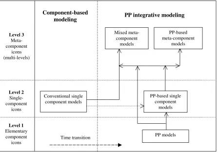
complex systems (imagine a direct-fired absorption chiller). Clearly, it is neither economical nor practical to model all equipment types on the basis of first-principle considerations. The mixing of model types through the adoption of appropriate data structures and classifications is illustrated in Figure 3.

For a given simulation task, it is expected that the model developer will possess technical knowledge about the available plant component models and the 27 PP models in terms of the physical laws they represent. The problem in hand (i.e. the physical plant system) may then be converted into a simulation model by selection of pre-constructed conventional component models, pre-constructed PP-based component models and new component models synthesized from PPs. To synthesize a new component model, the user might unpack an existing PP-based component model and adapt it to accommodate the present need. The process of unpacking exposes the model's constituent PP parts. These parts may then be replaced, modified (e.g. a parameter edited or a link changed) and/or augmented by the addition of new PPs. The finished (repacked) component model is endowed with a new icon and transferred back to the plant component library to be available for user selection against an appropriate classification (air-side, water-side, steam, refrigerant, solar etc). It is possible to envisage a future state where all plant component models are built automatically from PPs based on user mechanical descriptions. Such an approach to plant modeling would then be similar to that employed at present for building modeling: buildings of arbitrary complexity are synthesized, on the basis of architectural descriptions, from building-side PP process models representing wall conduction, inter-surface radiation exchange, air movement and the like.

AUTO-CONNECTION

The theoretical basis of PP modeling technique have been fully explained in Chow & Clarke 1998. By that time the coefficient generators of the plant components (via the addition of PP coefficients) were worked out manually at the source code level, making use of the ESP-r plant database as a testing platform. Recent efforts have been spending on the development of data structure and graphics that facilitates PP auto-connection via computer interface.

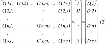
In a given problem, a typical PP matrix template with three nodes I, J and L is in the following format:

where k represents the kth primitive part selected in the defined problem; i, j and l represent numerically the node order of I, J and L in the overall matrix.

The global matrix of an overall system with ‘S’ number of nodes can be represented by:

                    =                     ×                     ) s ( D : ) n ( D : ) 2 ( D ) 1 ( D S : II I ) s , s ( C .. ) m , s ( C .. .. ) 1 , s ( C : : : ) s , n ( C .. ) m , n ( C .. .. ) 1 , n ( C : : : ) s , 2 ( C : ) 1 , 2 ( C ) s , 1 ( C .. ) m , 1 ( C .. ) 2 , 1 ( C ) 1 , 1 ( C (2)

In the equation, C(n,m) and D(n) represent the future time step and present time step coefficients in the global matrix respectively. According to the super-imposition rule, the matrix coefficients C(n,m) and D(n) can be given by the summation of PP coefficients, i.e.

∑

C (3)

∑

D (4)

The data structure can support different assigned node order and can arrive at the same required values of the overall matrix coefficients. In a specific simulation task, the program identifies the coefficients index of auto-connected PP and dynamically set the matrix coefficients in the course of simulation.

COOLING COIL MODELS

Consider a 4-row, counter-flow, chilled-water cooling coil represented by a nodal structure as shown in Figure 4. This example is used to illustrate the construction of a PP model. The coil comprises two headers, each for chilled water supply and return. There are two steps in the model construction process:

1. Synthesis of a model for the heat transfer tube (i.e. for each row of the coil) to give a PP-based component model; and

2. Use of this initial model together with additional PPs to synthesis of a model of the entire cooling coil.

A heat transfer tube can be synthesized using two 'flow upon surface' PPs: PP4.4 (for moist air; 2 nodes) and PP4.3 (for a single phase fluid; 3 nodes). These two icons are selected from the available PPs. Because the solid nodes of these two PPs are identical, they are merged into a single node by a special linking process (Figure 5). Built-in connection rules are invoked in order to check

connection validity, e.g. to ensure that the connection is between PP nodes of similar type. At this stage, the user must specify the technical parameters required by the selected PPs. These data are node-related as opposed to component-related. Examples include physical dimensions (such as length and volume), material properties (such as thermal conductivity, density and specific heat) and heat/mass transfer coefficients at various temperature and flow conditions. Where appropriate, default values and typical ranges for these input parameters are embedded within the user interface. To complete this part of the process, an icon is generated for the heat transfer tube model and is placed within the 'air-side' components menu of the plant library.

In the second stage, 4 PP5.2 'flow multiplier' icons and 4 heat transfer tube icons are selected (from separate menus) and used to complete the cooling coil model construction. These icons, on selection, are assigned to different addresses within the data structure of the new component model. Two PP5.2 models represent the incoming nodes of the supply air and water respectively, assuming uniform flow distribution to each coil layer. The remaining two PP5.2 models represent the collection of the flows from all layers to form two exiting streams of air and water respectively. The four heat transfer tube models are connected in series with the incoming and leaving flow multipliers. After the insertion of additional technical data, a new icon of the chilled water cooling coil model is generated and then located within the 'air-side' components menu.

The use of heat transfer tubes allows the cooling coil model to be constructed as an explicit representation of the actual device. To facilitate editing, say the conversion of the coil to parallel flow, the cooling coil model may be unpacked to expose the 4 PP5.2, the 4 heat transfer tube models and their linkages. The 'pack' process then converts the model and reassigns it to a new icon (Figure 3b). The process is fully extensible: for example, a steam-heating coil model may be constructed from a combination of the heat transfer tube model after modification to represent two-phase flow. In this case, the existing heat transfer tube model is unpacked to expose the PP4.3 sub-model. This sub-model is replaced by a PP4.2 (for 2-phase fluid; 3 nodes), with new technical data inserted. The model is repacked and associated with a new icon. Where the steam-heating coil involves a more complex tube arrangement then that can be supported by PP5.2, a PP5.1 may be used to model the new branch flows.

DATA STRUCTURE AND WORKFLOW

line' procedure employed as the backbone of complicated PP-based system simulation, with 'splitter' and 'mixer' introduced as two key concepts. The synthesis of a plant component may involve multiple parallel branches of PPs. In each branch, there should be only one mixer/splitter pair in the workflow. The main flow line may be divided into branches between mixer and splitter for organizational clarity and simulation logistics. This also allows for better handling of information flow. The splitter arranges all the data in order, and abstracts the general data entities in the global parameter database. The mixer collects the information and requests input from the user where conflicts arise.

Data are stored as a flow line image of the model building process. The model structure starts with input data, assisted by the mixer and splitter in branch connections. In this way, complicated information, such as the detailed compositions of a PP-based single component model, can be hidden from the user during the subsequent model applications and simulation runs. The data structure in program development can also be optimized.

CONCLUSION

PP modeling is an attempt to overcome the restrictions inherent in traditional component-based plant modeling. Its flexibility and generic nature makes the approach well adapted for use within integrative simulation environments. An appropriate data structure allows its mixed use with conventional component models. Using a chilled-water cooling coil as an example, the concept has been illustrated and discussed. Also introduced was the notion of 'work flow lines' whereby branch connections may be handled. It is envisaged that the PP technique could gradually replace the conventional approach to plant modeling in an attempt to unify the methods applied to the building and plant domains.

ACKNOWLEDGMENT

The authors express their thanks for the financial support of Strategic Research Grant 7001114 from the City University of Hong Kong.

REFERENCES

Buhl WF, Erdem FC, Winkelmann FC, Sowell EF. 1993. Recent improvements in SPARK: strong component decomposition, multivalued objects, and graphical interface, Proceedings of Building Simulation ‘93, the 3th International IBPSA Conference, Aug 16-18, Adelaide, Australia, pp.283-289.

Chow TT. 1995. Generalization in plant component modelling. Proceedings of Building Simulation '95, the 4th IBPSA International Conference, Madison, USA, August, pp.48-55.

Chow TT, Clarke JA. 1998. Theoretical basis of primitive part modeling. ASHRAE Transactions; 104(2): 299-312.

Chow TT, Clarke JA, Dunn A. 1997. Primitive parts: an approach to air-conditioning component modeling, Energy and Buildings; 26: 165-173. Clarke JA. 1999. Prospects for truly integrated

building performance simulation, Proceedings of Building Simulation ’99, the 6th International IBPSA Conference, Sep, Kyoto, Japan, Vol.3, pp.1147-1154.

Crawley DB et al. 2001. ENERGYPLUS: New capabilities in a whole-building energy simulation program, Proceedings of Building Simulation 2001, the 7th International IBPSA Conference, Aug, Rio de Janeiro, Brazil, Vol.1, pp.51-58.

ESRU. 2000. ESP-r: a building and plant energy simulation environment: user guide version 9 series, University of Strathclyde, Glasgow. Sahlin P, Bring A, Kolsaker K. 1995. Future trends of

the Neutral Model Format (NMF), Proceedings of Building Simulation ‘95, the 4th International IBPSA Conference, Aug 14-16, Madison, Wisconsin, USA, pp.537-544.

Sahlin P. 1993. IDA modeler, a man-model interface for building simulation, Proceedings of Building Simulation ‘93, the 3th International IBPSA Conference, Aug, Adelaide, Australia, pp.299-305.

Name Description Environment data ! Boundary conditions

! Input/output data

! Project information Parameter data ! Component or PP

parameters

! Component initial data Connection data ! Connection

! Workflow pointer

! Pack and unpack information

Primitive parts:

1 Thermal conduction 1.1 solid to solid 1.2 with ambient solid

2 Surface convection 2.1 with moist air

2.2 with 2-phase fluid 2.3 with 1-phase fluid 2.4 with ambient

3 Surface radiation 3.1 with local surface 3.2 with ambient surface

4 Flow upon surface 4.1 for moist air; 3 nodes 4.2 for 2-phase fluid; 3 nodes 4.3 for 1-phase fluid; 3 nodes 4.4 for moist air; 2 nodes 4.5 for 1-phase fluid; 2 nodes

5 Flow divider and inducer 5.1 Flow diverger (for all fluid) 5.2 Flow multiplier (for all fluid) 5.3 Flow inducer (for all fluid)

6 Flow converger 6.1 for moist air 6.2 for 2-phase fluid 6.3 for 1-phase fluid

6.4 for leak-in moist air from outside

7 Flow upon water spray 7.1 for moist air

8 Fluid injection 8.1 water/steam to moist air

9 Fluid accumulator 9.1 for moist air

9.2 for liquid

10 Heat injection 10.1 to solid

10.2 to vapor-generating fluid 10.3 to moist air

PP2.2 PP2.3 PP2.4

PP3.1 PP3.2 PP4.1

PP4.2 PP4.3 PP4.4

PP4.5 PP5.1 PP5.2

PP8.1 PP9.1 PP9.2

PP5.3 PP6.1 PP6.2

PP6.3 PP6.4 PP7.1

PP10.1 PP10.2 PP10.3

PP1.1 PP1.2 PP2.1

Figure 1 List of primitive part icons Table 1

Figure 2 Integrative simulation environment

Project Manager graphic, CAD and expert systems

Building Models

Plant Models

Fluid Flow Models

Lighting Models

Power Flow Models

Control Models

Comfort Condition

Indoor Air Quality

Energy Use

Optimal Design Weather

Definitions

Building Definitions

HVAC Definitions

Lighting Definitions

Central Database

Result Recovery

Inputs Simulation Core Outputs

form and fabric

components and connections

velocity and pressure

luminance and colour

conversion and storage

construction, plant, climate and generic libraries

summary, tabulation, and statistical procedures Human

Models

Computation Models

numerical and analysis techniques activities and physiology devices and algorithms Performance

Criteria

Figure 3 Plant component library structure Air

Cooling Coil

Heat Transfer Tube

PP4.4, PP4.3 Meta

Single

PP

Level 3

Level 2

Level 1 Pack

Pack

Unpack

Unpack

(b) Component structure (a) Hierarchy of PP models Conventional single

component models

PP-based single component

models

PP models PP-based meta-component

models Mixed meta-

component models

Time transition

Component-based

modeling

PP integrative modeling

Level 3 Meta-component

icons (multi-levels)

Level 2 Single-component

icons

Level 1 Elementary component

Figure 4 A 4-row chilled-water cooling coil

A0

A1

A2

A3

A4

W0

W2

W4

W3

W1

S1

S2

S3

S4

WM 4

WM3

WM2

WM1

chilled water

air

Node

Name/Identifier

Node type Entity node type

Name in database Identifier

Nodes list PP parameters Connection identifier

Code

Identifier

Supply/Demand/Output Component list

Node

Primitive Part

Component

Node Connec

tion

P

P

Connec

tion

PP Component Data Structure PP Modeling Environment

Environment Parameter Connection

Tube