network for maritime applications utilizing a distributed parallel algorithm
.
White Rose Research Online URL for this paper:
http://eprints.whiterose.ac.uk/150626/
Version: Accepted Version
Article:
Cao, B., Zhao, J., Yang, P. orcid.org/0000-0002-8553-7127 et al. (3 more authors) (2018)
3-D multiobjective deployment of an industrial wireless sensor network for maritime
applications utilizing a distributed parallel algorithm. IEEE Transactions on Industrial
Informatics, 14 (12). pp. 5487-5495. ISSN 1551-3203
https://doi.org/10.1109/tii.2018.2803758
© 2018 IEEE. Personal use of this material is permitted. Permission from IEEE must be
obtained for all other users, including reprinting/ republishing this material for advertising or
promotional purposes, creating new collective works for resale or redistribution to servers
or lists, or reuse of any copyrighted components of this work in other works. Reproduced
in accordance with the publisher's self-archiving policy.
[email protected] https://eprints.whiterose.ac.uk/ Reuse
Items deposited in White Rose Research Online are protected by copyright, with all rights reserved unless indicated otherwise. They may be downloaded and/or printed for private study, or other acts as permitted by national copyright laws. The publisher or other rights holders may allow further reproduction and re-use of the full text version. This is indicated by the licence information on the White Rose Research Online record for the item.
Takedown
If you consider content in White Rose Research Online to be in breach of UK law, please notify us by
Sensor Network for Maritime Applications Utilizing a Distributed Parallel Algorithm
.
White Rose Research Online URL for this paper:
http://eprints.whiterose.ac.uk/150626/
Version: Accepted Version
Article:
Cao, B orcid.o
rg/0000-0003-4558-9501, Zhao, J, Yang, P orcid.org/0000-0002-8553-7127
et al. (3 more authors) (2018) 3-D Multiobjective Deployment of an Industrial Wireless
Sensor Network for Maritime Applications Utilizing a Distributed Parallel Algorithm. IEEE
Transactions on Industrial Informatics, 14 (12). pp. 5487-5495. ISSN 1551-3203
https://doi.org/10.1109/tii.2018.2803758
[email protected] https://eprints.whiterose.ac.uk/ Reuse
Items deposited in White Rose Research Online are protected by copyright, with all rights reserved unless indicated otherwise. They may be downloaded and/or printed for private study, or other acts as permitted by national copyright laws. The publisher or other rights holders may allow further reproduction and re-use of the full text version. This is indicated by the licence information on the White Rose Research Online record for the item.
Takedown
If you consider content in White Rose Research Online to be in breach of UK law, please notify us by
Abstract—Effective monitoring marine environment has become a vital problem in the marine applications. Traditionally, marine application mostly utilizes oceanographic research vessel methods to monitor the environment and human parameters. But these methods are usually expensive and time-consuming, also limited resolution in time and space. Due to easy deployment and cost-effective, WSNs have recently been considered as a promising alternative for next generation IMGs. This paper focuses on solving the issue of 3D WSN deployment in a 3D engine room space of a very large crude-oil carrier (VLCC), in which many power devices are also considered. To address this 3D WSN deployment problem for maritime applications, a 3D uncertain coverage model is proposed with a new 3D sensing model and an uncertain fusion operator, is presented. The deployment problem is converted into a multi-objective problems (MOP) in which three objectives are simultaneously considered: Coverage, Lifetime and Reliability. Our aim is to achieve extensive Coverage, long Lifetime and high Reliability. We also propose a distributed parallel cooperative co-evolutionary multi-objective large-scale evolutionary algorithm (DPCCMOLSEA) for maritime applications. In the simulation experiments, the effectiveness of this algorithm is verified in comparing with five state-of-the-art algorithms. The numerical outputs demonstrate that the proposed method performs the best with respect to both optimization performance and computation time.
Index Terms—wireless sensor network deployment, 3D engine room, Very large crude-oil carrier (VLCC), Coverage, Lifetime, Reliability, Parallel, Multi-objective evolutionary algorithm.
I. INTRODUCTION
S the increasing human activities being undertaken in the marine environment, effective and efficient monitoring marine environment has become a vital problem in the industrial applications. Traditionally, marine application mostly utilizes oceanographic research vessel methods [1-2] to monitor the environment and human parameters. But these methods are usually expensive and time-consuming, also limited resolution in time and space. Recently, due to the advantages of automatic operation, easy-deployment, real-time mode and cost-effective, industrial wireless sensor network (WSNs) have recently been
considered as promising alternative for next generation intelligent maritime grid (IMG) applications. Many studies have been conducted on industrial WSNs for marine environment monitoring, including sensors design and deployments [3], systems architecture and efficiency [4-5], communication and optimisation techniques [6-7], etc.
Among these issues, the deployment problem of WSNs is a foundamental challenge for operational management and security monitoring of Intelligent Maritime Grids (IMGs). But so far most existing current research in WSNs assumes that these networks are deployed in a terrestrial 2D environment, and can be optimised by applying probabilistic fusion operator [11-14] with omni-directional 2D sensing models, like the disk/Boolean sensing model [8], the Elfes sensing model [9] and the Li sensing model [10]. While above methods have demonstrated promising performances on dealing with the traditional coverage optimisation problem in ideal 2D WSN environment, it is still difficult to achieve practical needs of WSN deployment in real word 3D cases. Especially, for many maritime application,
This paper aims at exploring the possibility of utilising biological inspired optimisation algorithms to efficiently solve the coverage problem in 3D WSNs for maritime application. In this paper, we study the 3D deployment problem of an IWSN in a 3D engine room space of a very large crudeoil carrier (VLCC), in which there are many power devices. To better consider the coverage problem, we propose a 3D directional sensing model by simultaneously considering the sensing distance and horizontal and vertical sensing angles, which is probabilistic to improve precision and practicability. Also, our model has considered supporting heterogeneous directional sensor nodes [21] with improved practicability.
In this paper, we inspired from the idea of particle swarm optimisation [22] and simultaneously deploy sensor nodes and relay nodes. Consequently, the energy consumptions of relay nodes are balanced to maximize the lifetime. For an IWSN, reliability is also crucial. In the work of [23], Wang et al. guaranteed reliability by ensuring the associations of each node to multiple relay nodes. In this paper, we also consider the reliability of the IWSN. Instead of making the reliability objective a constraint, we transform it into an objective to be optimized. Due to the fact that this model has considered three above objectives simultaneously, the deployment problem can
3D Multi-Objective Deployment of an Industrial
Wireless Sensor Network for Maritime
Applications Utilizing a Distributed Parallel
Algorithm
Bin Cao, Jianwei Zhao, Po Yang*, Zhihan Lv
be characterized as a multi-objective optimization problem (MOP). Thus, we use multi-objective evolutionary algorithms (MOEAs) to address the deployment problem. Hacioglu et al. [24] considered multiple aspects of energy consumption, and Non-dominated Sorting Genetic Algorithm II (NSGA-II) [25] was applied. In the work of [24], Jameii et al. simultaneously considered coverage, energy consumption and the number of active sensors, and NSGA-II was also utilized. Sengupta et al. [26] formulated the deployment problem with respect to three aspects: lifetime objective, coverage objective and the connectivity constraint; to solve this MOP, they blended fuzzy Pareto dominance with Multi-objective Evolutionary Algorithm Based on Decomposition (MOEA/D) [27], therein proposing MOEA/DFD, which outperformed popular MOEAs and several single-objective evolutionary algorithms (EAs). However, the above works only considered the 2D scenario; to our knowledge, studies having utilized MOEAs to solve the 3D engine room space deployment problem for maritime applications are rare. The main contributions of this paper are:
1. For the operational management and security monitoring of Intelligent Maritime Grids (IMGs), a novel WSN coverage model with a 3D sensing model and an uncertain fusion operator is proposed for 3D engine room in practical maritime applications.
2. We consider the deployment problem with heterogeneous sensors in a 3D engine room space of a VLCC, in which many power devices are also considered. The deployment in 3D WSN for maritime applications is transformed into a multi-objective deployment problem with simultaneous consideration of Coverage, Lifetime and Reliability. 3. An evolutionary optimization algorithm is proposed and
evaluated for solving above problem. A modified MOEA, distributed parallel cooperative co-evolutionary multi-objective large-scale evolutionary algorithm (DPCCMOLSEA), is proposed; in addition to reduce the computation time, MPI (message passing interface) parallelism is utilized.
The remainder of this paper is organized as follows. Section II describes the 3D engine room deployment problem and related preliminaries. We provide a detailed introduction to the proposed novel 3D uncertain coverage model in Section III. Section IV describes the three objective functions considered, details the Lifetime and Reliability objectives and provides the representation of individuals in the population for the MOEAs. The proposed algorithm is presented in Section V. We report our experimental simulations and analyses in Section VI, and the paper is concluded in Section VII.
II. LITERATURE REVIEW
During the last few years, WSNs (wireless sensor network) have been widely studied and utilised in many industrial applications, related to forest monitoring [28], agriculture monitoring [29], and healthcare [30-31]. Compared to the practical working environment of above applications, marine environment systems are quite sensitive to the effects of human activities. Traditionally, marine application mostly utilizes oceanographic research vessel methods [1-2] to monitor the environment and human parameters. But these methods are usually expensive and
time-consuming, also limited resolution in time and space. For marine environment research, a WSN-based approach can dramatically improve the access to real-time data covering long periods and large geographical areas [32]. According to Tateson et al. [33], a WSN-based approach is at least one order of magnitude cheaper than a conventional oceanographic research vessel.
Typically, a WSN-based marine system needs to measure different physical and chemical parameters. While the development and deployment of an adaptive, scalable and self-healing WSN system need to address a number of critical challenges such as autonomy, scalability, adaptability, self-healing and simplicity [34], the design and deployment of a lasting and scalable WSN for marine environment monitoring should take into account the following challenges different from those on land [35]: stronger robustness, higher energy consumption, and sensor coverage problem, maintenance of sensor nodes.
There are many concerns relevant to the deployment problem, one of which is coverage [36-37]. The authors of [38] simultaneously considered connectivity, cost and lifetime. Similarly, in the present paper, in addition to the 3D space coverage, we also consider the lifetime of the IWSN. To prolong the lifetime, Kuila et al. [39] utilized a heterogeneous structure that contained both sensor nodes and relay nodes simultaneously. The energy consumptions of different types of nodes were considered simultaneously. The energy consumed by each relay node was comprehensively balanced with respect to the sensor nodes that it was in charge of, data aggregation, and extra energy consumption by acting as a hop node for other relay nodes. Consequently, the overall lifetime could be prolonged to a large extent.
Among these studies, the deployment problem of WSNs is a key issue for operational management and security monitoring of Intelligent Maritime Grids (IMGs). Traditional sensing models for 2-D sensor nodes are omni-directional and include the disk/Boolean sensing model [8], the Elfes sensing model [9] and the Li sensing model [10]. The most common fusion operator is the probabilistic fusion operator [11-12]. The traditional coverage models of WSNs are based on probability measures such as those in the problems of certain coverage discussed in [13-14]. While above studies have demonstrated promising performances on dealing with the coverage optimisation in ideal 2D WSN environment, it is still difficult to achieve practical needs of WSN deployment in real word 3D cases. However, most existing deployment strategies in WSNs focus on ideal 2D WSN environment, which are hardly to be applied in real maritime application environments. The sensing models considered in traditional maritime wireless sensor networks (MWSNs) [15-17] are very simple, mostly with the deployment on a 2D plane.
above a 3D terrain. However, the above studies did not consider network lifetime or energy consumption [20]. In real-world marine environment application, sensor nodes in WSNs have limited battery power. The energy consumption of sensor nodes is important for sensor networks. The lifetime is a result of energy consumption in WSNs. Consequently, so far there are no existing practically efficient solutions in literature for dealing with coverage and deployment problems in complex 3D surface of WSNs in marine environment application.
This paper aims at exploring the possibility of utilising biological inspired optimisation algorithms to efficiently solve the coverage problem in 3D WSNs for maritime application. In this paper, we study the 3D deployment problem of an IWSN in a 3D engine room space of a very large crudeoil carrier (VLCC), in which there are many power devices. To better consider the coverage problem, we propose a 3D directional sensing model by simultaneously considering the sensing distance and horizontal and vertical sensing angles, which is probabilistic to improve precision and practicability. Also, our model has considered supporting heterogeneous directional sensor nodes [21] with improved practicability.
In this paper, we inspired from the idea of particle swarm optimisation [22] and simultaneously deploy sensor nodes and relay nodes. Consequently, the energy consumptions of relay nodes are balanced to maximize the lifetime. For an IWSN, reliability is also crucial. In the work of [23], Wang et al. guaranteed reliability by ensuring the associations of each node to multiple relay nodes. In this paper, we also consider the reliability of the IWSN. Instead of making the reliability objective a constraint, we transform it into an objective to be optimized. Due to the fact that this model has considered three above objectives simultaneously, the deployment problem can be characterized as a multi-objective optimization problem (MOP). Thus, we use multi-objective evolutionary algorithms (MOEAs) to address the deployment problem. Hacioglu et al. [24] considered multiple aspects of energy consumption, and Non-dominated Sorting Genetic Algorithm II (NSGA-II) [25] was applied. In the work of [24], Jameii et al. simultaneously considered coverage, energy consumption and the number of active sensors, and NSGA-II was also utilized. Sengupta et al. [26] formulated the deployment problem with respect to three aspects: lifetime objective, coverage objective and the connectivity constraint; to solve this MOP, they blended fuzzy Pareto dominance with Multi-objective Evolutionary Algorithm Based on Decomposition (MOEA/D) [27], therein proposing MOEA/DFD, which outperformed popular MOEAs and several single-objective evolutionary algorithms (EAs). However, the above works only considered the 2D scenario; to our knowledge, studies having utilized MOEAs to solve the 3D engine room space deployment problem for maritime applications are rare.
III. PRELIMINARIES AND PROBLEM SIMULATION
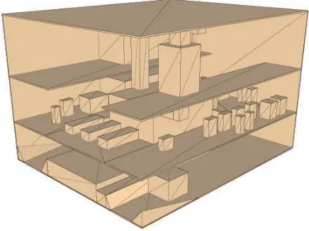
For the maritime application, we regard the 3D engine room space of a VLCC as a cuboid, inside of which devices are represented by smaller cuboids, as shown in Fig. 1. To perform the mathematical simulation, we discretize the engine room space, and a 3D matrix is constructed, in which 0 represents free space and 1 denotes obstacles (e.g., devices, bulkheads and
[image:5.612.322.540.81.244.2]upper decks).
Fig. 1 Engine room model of a VLCC
A. Line of Sight (LOS)
For a sensor s attempting to observe a target point t in 3D space, if no obstacle blocks the sight line joining them, then s and t can
“see” each other, and we say that there exists a Line of Sight
(LOS); otherwise, the No Line of Sight (NLOS) condition prevails between them. The LOS condition is a prerequisite for sensor s to be able to detect point t.
B. Deployment Positions
1) Sensor Nodes: We restrict the deployment positions of the wireless sensors, that is, directional wireless sensors are deployed at the bulkheads and the upper decks of the engine room. However, not all position points are feasible (e.g., obstacles exist). To restrict the coordinates of the points, we utilize a penalty ps:
infeasible S
psn penalty (1)
Where ninfeasibleS is the number of infeasible sensor positions and penalty denotes the penalty parameter, which is assigned a huge value (e.g., 106).
2) Relay Nodes: For the relay nodes, because they collect messages from directional sensors, they are also deployed at the bulkheads and the upper decks. Similarly, we also have a penalty pR for the relay nodes:
infeasible R
pRn penalty (2)
Where ninfeasibleR is the number of infeasible points of the relay
node deployment.
IV. UNCERTAIN COVERAGE MODEL
A. Sensing Model
In a 3D space, the sensing probabilityPS( , )s t of a sensor s to a target point t can be calculated as given by the equation below:
( , ) ( , ) ( , ) ( , ) ( , )
S S S S S
LOS D P T
P s t P s t P s t P s t P s t (3)
Where PDS( , )s t , PPS( , )s t and PTS( , )s t are the sensing probabilities associated with the sensing distance, horizontal sensing angle and vertical sensing angle, respectively, and
( , )
S LOS
P s t is a two-valued function with the following form: 1, if LOS
( , )
0, if NLOS
S LOS
P s t
(4)
Below, we first describe the distance sensing model and then the angle sensing model.
1) Distance-based Sensing Model: The Li sensing model [10] is used. Let the deterministic sensing distance be denoted by Rd,
and let the fuzzy distance be Rf. The mathematical
representation is as follows
1 2 1 1 2 2
( / + )
1, ( , ) [0, ]
( , ) , ( , ) [ , ]
0, ( , ) [ , ]
d
r r
S
D d d f
d f
r s t R
P s t e r s t R R R
r s t R R
(5)
Wherer1r s t( , )Rd ; r2 Rd Rf r s t( , );
1, 2, 1and2
are parameters; and sensors with various characteristics can be simulated by adjusting their values.2) Angular Sensing Model: We consider two angular sensing dimensions: the horizontal angular range and the vertical angular range. By first calculating the sensing probabilities with respect to these two angles, we can obtain the sensing probabilities corresponding to different 3D angles.
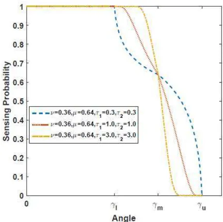
The sensing behaviours with respect to both angles are similar. We define three angle thresholds,lX, mXand uX, where lXmXuX, and X denotes PAN or TILT, referring to horizontal or vertical directions, respectively. This model can be described as follows:
1
1 ( )
( , )
1
1 ( )
( , )
1, ( , ) [0, ]
( , ) 1 , ( , ) [ , ]
, ( , ) [ , ]
0
0, ( , ) [ , ]
X
X l
X X X
m l
X s t
S X X l X X
X X l m
X X X
m l
X X X
s t
X X l
X m u
X
X u
s t
P s t v e s t
s t e s t (6) . . X( , ) X X( , )
s t s t rt s t
Where
X( , )s t is the deflection angle;
X( , )s t is its modified value; rtXis the modification ratio;
X,X, 1X
and 2 X
[image:6.612.321.551.150.379.2] are parameters used to simulate different sensing characteristics; and vXX 1, vX,X[0,1] . For different parameter values, the characteristics of the model are shown in Fig.2.
Fig. 2 Characteristics of the angular sensing model
B. Uncertain Fusion Operator
At a given point t in 3D space, the sensing regions of multiple sensors may overlap. The traditional method for addressing this situation is based on the additivity of probability. However, in a practical environment, various sources of interference may exist, and consequently, the sensing probability may not be additive. Therefore, we utilize the Sugeno measure [40] to simulate the fused sensing behavior of multiple sensors. For the sensor set
1 2
{ , ,..., Ns}
S s s s (where NS is the number of sensors), we can
calculate their fused sensing probability PSF( )t for point t as follows:
1
1
( ) min(1, { [1 ( , )] 1})
Ns
F S
S k
k
P t P s t
(7)Where
1 0is an adjustable parameter that is used
to simulate different environment. The Sugeno measure
is a type of non-probabilistic measure that possesses the
characteristic of weak additivity, and when
1, the
Sugeno measure becomes a probabilistic measure.
To determine whether t can be detected, we define a
threshold
Fth
P
to convert the sensing probability
( )
F S
1, ( ) ( )
0,
F F
BF S th
S
P t P
P t
otherwise
(8)
The quality of coverage (QoC) can be defined as the average coverage degree of the entire 3D space:
1 1 ( ) N BF S k k
QoC P t
N
(9)Where N is the number of considered discrete points in the 3D space.
V. OPTIMIZATION OBJECTIVES AND REPRESENTATION OF
INDIVIDUALS IN THE POPULATION
The deployment problem is converted into an MOP by simultaneously considering the calculation of the QoC, the lifetime and the reliability. For the optimization, MOEAs are utilized. In the following, we will discuss these issues in detail.
A. Coverage
We need to guarantee the extensive coverage of the 3D engine room space. Let fCoveragedenote the value of the objective function for Coverage. It has the following form:
1.0
Coverage
f QoC (10)
B. Lifetime
According to the radio model for energy consumption introduced in [29], we have
2 0 4 0 , ( , ) , d d fs th t d d d mp th
l E l d d d
E l d
l E l d d d
(11)
And
0
( )
r d d
E l l E (12)
Where Et and Er are the energy used for transmitting and
receiving messages, respectively; ld is the length of a message; d
is the distance between the transmitter and the receiver; dth is the
threshold determining the adoption of the freespace model (fs) or the multipath model (mp); E0 represents the electronics
energy; and fsand mp are the amplifier energy parameters for the above two models, respectively.
The lifetime issue [38] mainly considers the relay nodes, which is detailed as follows:
The relay nodes gather messages from sensor nodes and transmit them to the sink node directly or indirectly using other relay nodes as hop nodes. Thus, we should balance the energy consumptions by comprehensively considering the number of messages and the transmission distances. Simply, the nearest relay node nearer to the sink node is chosen as the next hop of the current relay node; otherwise, messages are directly transferred to the sink node.
Therefore, the objective function for the Lifetime objective,
Lifetime
f , has the following form:
min scale L Lifetime RN f L
(13)
where Lscaleis a scale value used to guarantee that the value of
Lifetime
f is within [0; 1), which is set to 104, and
min RN
L is the minimum lifetime of all relay nodes.
C. Reliability
Based on the work of [21], we transform the reliability constraint into an objective that can be optimized. Assuming that each sensor or relay node is connected to NRreliarelay nodes, the fitness of the Reliability objective is as follows:
1 1 Re / / R Ns N S R R i i i i liability scale R
d Ns d N
f
(14)where diS denotes the average distance of sensor node i to its nearest NRreliarelay nodes, diR is that distance with respect to relay node i, NR is the number of relay node, and Rscale is a
scale value.
D. Representation of Individuals in the Population
Because there are three rooms (Fig. 1) and because nodes can be deployed at the bulkheads and upper deck of each room, an indicator is utilized to denote which plane (a total of 15 planes) is considered.
The directional sensor s can be represented by the five iS tuple (biS,xiS,yiS,iPAN,iTILT) . Here,
S i
b indicates the deployment plane, (xiS,yiS)denotes the position, and iPANand
TILT i
are the horizontal and vertical sensing angles, respectively. Each relay node s is represented by a three kR tuple (bkR,xkR,ykR). Here, b indicates the deployment plane, kR and (xkR,ykR)denotes the deployment position. Therefore, in the optimization algorithm, the set of all individuals in the population can be represented by( 1,..., , 1 ,..., )
S S R R
Ns NR
s s s s , whose dimension nDim is Ns 5 NR3.
VI. PROPOSED ALGORITHM
species. Moreover, the computational burden of each species is allocated to the CPU resources.
A. Overall Structure
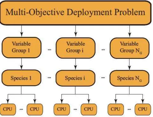
The pseudocode of DPCCMOLSEA is provided in Alg.1, and the overall structure is illustrated in Fig. 3. Similar to our previous proposed algorithm Distributed Parallel Cooperative Coevolutionary Multi-objective Evolutionary Algorithm (DPCCMOEA) [41], variables are separated into several groups, where each group is optimized by a species. However, for the second layer, in DPCCMOEA, individuals are further allocated to the CPUs owned by each species, and each CPU is in charge of the evolution and fitness evaluations of individuals. For the proposed DPCCMOLSEA, in each species, a master CPU is responsible for the evolution of the individuals, while the computational burden of fitness evaluations is shared by all the CPUs. The difference is in, in the lower layer, whether the evolution of individuals is conducted by a single master CPU or delegated to all CPUs.
Algorithm 1: DPCCMOLSEA
1. Separate large numbers of variables to several groups: 2. Uniformly distribute all MPI resources to all groups;
3. From a species in the master CPU for each group;
4. While The number of fitness evaluations is not exhausted Do
/* Evolution */
5. Evolve the variables in the group in each master CPU in
serial for all groups in parallel;
/* Crossover */
6.Remaining variables are generated through crossover;
/* Evaluation */
7.Master CPUs allocate the generated offsprings, the
fitness evaluations are performed in parallel in all CPUs, and the fitness values are collected to the master CPUs;
/* Updating subpopulations
*/
8.In the master CPUs, based on the fitness values of the generated offsprings, update the species;
/* Synchronizing subpopulations
*/
9.All master CPUs communicate with each other;
[image:8.612.317.565.55.245.2]10. Gather individuals in all species, and generate the final population by selecting the best individuals
Fig. 3 Organisation of DPCCMOLSEA for the considered problem
B. Optimisation
The evolution pattern of DPCCMOEA, borrowed from MOEA/D [42], is inherited by DPCCMOLSEA. Thus, each individual refers its neighbourhood for evolution. In DPCCMOEA,as individuals in each species are separated into several sets, the neighbourhood relationship is cut off; the updating process also concerns the neighbourhood, which is also disrupted. In contrast, DPCCMOLSEA performs the evolution of all individuals of a species in a single master CPU, which is the same as in serial algorithms, thus comprehensively taking advantage of mutual relations among individuals for the whole species.
C. Crossover
Each species optimizes a group of variables, and differential evolution (DE) [43] is the optimizer used; specifically, DE/rand/1 is the detailed form in DPCCMOEA, while in DPCCMOLSEA, we also experiment with jDE [44] and JADE [45], denoted as DPCCMOLSEA-jDE and DPCCMOLSEAJADE, respectively.
For convenience, each species stores the other variables as well as the optimized variables. To form a complete solution, the remaining variables should be integrated. For this, we use crossover, that is, all the evolved variables in the current optimized group are reserved in the generated offspring, while the stored parent and other selected stored solutions are utilized to generate the remaining variables through crossover. In DPCCMOEA, half of the remaining variables come from the stored parent. In DPCCMOLSEA, we use a fixed value of 0:5 for DE/rand/1 and the corresponding adaptive strategies for jDE and JADE.
VII. EXPERIMENTAL SIMULATION AND ANALYSIS
A. Experimental Setup
[image:9.612.316.550.71.265.2] [image:9.612.317.550.291.454.2]The parameter settings for the coverage model are listed in Table I. The proposed algorithm is compared with five MOEAs: Cooperative Coevolutionary Generalized Differential Evolution 3 (CCGDE3) [46], MOEA/D [42], Multi-Objective Evolutionary Algorithm Based on Decision Variable Analyses (MOEA/DVA) [47], NSGA-II [25] and DPCCMOEA [41]. Each algorithm runs 20 times, and the number of fitness evaluations (FEs) for each run is set to (ND x 5 + NR x 3) x 104.
All algorithms are implemented in C++, and the simulation experiment platform is the TianHe-2 supercomputer.
For a fair comparison, the population size (NP) for all algorithms is set to 120. The number of species in CCGDE3 is set to 2, and the species size is 60.
For the components of all algorithms, we summarize: 1. DE is used in CCGDE3, MOEA/D, MOEA/DVA,
DPCCMOEA and DPCCMOLSEA.
2. SBX and polynomial mutation are used in NSGA-II; polynomial mutation is used in MOEA/D, MOEA/DVA, DPCCMOEA and DPCCMOLSEAs.
3. MOEA/DVA, DPCCMOEA and DPCCMOLSEAs are based on the decomposition framework of MOEA/D. 4. Variable analysis and grouping are performed in
MOEA/DVA, DPCCMOEA and DPCCMOLSEAs. Correspondingly, the detailed parameter settings are summarized in Table II.
B. Results and Analysis
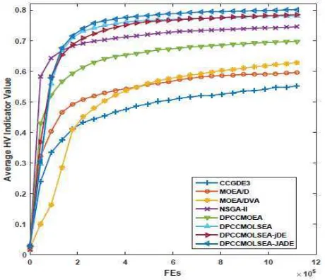
We use the hypervolume (HV) indicator [48] to evaluate the performance of the algorithms. A higher HV indicator value indicates a better optimization performance. In addition, the non-dominated solution sets are visualized.
Table III lists the statistical test results, including the rankings from the Friedman test and the Wilcoxon test with respect to the best algorithm, DPCCMOLSEA-JADE, from which we can see that DPCCMOLSEA-JADE is significantly better than all other algorithms (with p-values less than 0:05). When adopting different DE optimizers, the performance of DPCCMOLSEAs varies greatly: JADE is quite effective, while jDE is not very powerful, indistinguishable from DE/rand/1. The visualizations of all the non-dominated solutions generated from the 20 runs by each algorithm are provided in the supplementary material. We can see that DPCCMOLSEAs can comprehensively optimize all objectives.
Table IV lists the computation times of all the algorithms. We can see that because DPCCMOEA and DPCCMOLSEAs are parallel algorithms, their computation times are much lower. The speedup ratios are also calculated. The ratio values are approximately 79:6% s 87:1% of the ideal speedup (i.e., 72, which is the number of CPUs). DPCCMOLSEAs are slightly slower than DPCCMOEA, which can be ascribed to the parallel structure modification.
C. Time and Space Complexities
Table IV lists the computation time of all algorithms. As DPCCMOEA and DPCCMOLSEAs are parallel algorithms, their computation time is much lower. The speedup ratio values are approximately 79:6% s 87:1% of the ideal speedup (i.e., 72, which is the number of CPUs). DPCCMOLSEAs are slightly slower than DPCCMOEA, which can be ascribed to the parallel structure modification. T1 is the time consumption of fitness evaluations of the objective function, and T2-T1 provides the time consumptions of the algorithms without the fitness evaluations, viz., the time complexity of each algorithm.
And for each parallel algorithm, there are two values: the first one denotes the time consumption for one MPI process, while the second one between parentheses is the sum of time consumed by all MPI processes. As to the operation time, the time complexities of parallel algorithms are significantly lower than serial ones; however, if the time taken by all CPUs is considered, the serial ones are better, which can be attributed to the communication load in parallel algorithms.
For the space complexity, the population matters the most. MOEA/D, MOEA/DVA and NSGA-II are similar; in CCGDE3, variables are separated to two groups, correspondingly, there are two subpopulations, each of which stores the variable group and also the complete individuals with all variables, so there will be more space required; for all parallel algorithms, analogous to CCGDE3, corresponding to each group of variables, there is a species in the master CPU, while for the evaluation, there is extra space needed for the remaining CPUs, therefore, in total, the space is doubled. All in all, the space complexity is summarized as: parallel algorithms > CCGDE3 > other algorithms.
VIII. DISCUSSION
While the proposed novel 3D WSN coverage model with evolutionary optimisation algorithm has demonstrated a good performance in targeted objectives Coverage, Lifetime and Reliability for environment monitoring of Intelligent Maritime
applications, there are still other issues requiring further investigation.
The first issue is about the oceanographic sensor protection. Typical marine environments contains over thousands organisms related to fouling problems. When oceanographic sensors are immersed in seawater, they are susceptible to bio-fouling problems which often lead to the long-term accuracy issues of marine environmental sensor measurements. So our model should also consider this issue in our WSN coverage model.
[image:10.612.321.561.484.594.2]The second issue is about the limited energy of batteries of WSN in maritime system applications. In marine environment monitoring systems, wireless sensor nodes are often deployed in unapproachable sea surface areas, and they are mostly planned
Fig. 4 Evolutionary curves of average HV indicator values obtained by all algorithms
for long-time operation, therefore, it is not convenient to replace the sensor batteries. So our model should consider the following three aspects: energy harvesting devices, power management system, and energy storage devices.
IX. CONCLUSION
In this paper, for the operational management and security monitoring of Intelligent Maritime Grids (IMGs), we study the deployment of an IWSN in a 3D engine room space of a VLCC with many power devices. A novel 3D uncertain coverage model that consists of a sensing model and an uncertain fusion operator is proposed. This approach allows the Coverage to be calculated, and by simultaneously considering the Lifetime and Reliability objectives, we solve the deployment problem as an MOP. To address this MODP, we propose a novel method. Compared with several state-of-the-art algorithms, the proposed method performs the best with respect to both optimization performance and computation time (compared to serial algorithms only). In future work, other objectives can also be considered. Larger scale deployment problems can be tested, and the parallelism of the proposed algorithm can be further improved through implementation on GPUs or MICs.
REFERENCES
[1] J. Sorribas, J. D. Rio, E. Trullols, and A. Manuel-Lazaro, “A meteorological data distribution system using remote method invocation technology,” IEEE Trans. Instrum. Meas., vol. 55, no. 5, pp. 1794–1803, May. 2006. [2] S. Turkmen, B. Aktas, M. Atlar, N. Sasaki, R. Sampson, and W. Shi,
“On-board measurement techniques to quantify underwater radiated noise
level”, Ocean Engineering, vol. 130, pp. 166-175, January, 2017.
[3] A. Vermeij and A. Munafo, “A robust, opportunistic clock synchronization algorithm for Ad Hoc Underwater Acoustic Networks”, IEEE Journal of
Oceanic Engineering, vol.40, issue 4, pp. 841-852, April, 2015.
[4] P. Yang, W. Wu, M. Moniri, and C. C. Chibelushi, “Effective object localisation using sparsely distributed passive RFID tags”, IEEE Trans. Ind. Electron., vol. 60, no. 12, pp. 5914–5924, Sep. 2014.
[5] C. A. Perez, F. S. Valles, R. T. Sanchez, M.J.Buendia, F. Lopez-Castejon, J.
G. Ververa, “Design and deployment of a wireless sensor network for the mar menor coastal observation system”, IEEE Journal of Oceanic
Engineering, vol.42, issue 4, pp. 966-976, April, 2017.
[6] O. Kreibich, J. Neuzil, and R. Smid, “Quality-based multiple-sensor fusion
in an industrial wireless sensor network for MCM,” IEEE Trans. Ind. Electron., vol. 61, no. 9, pp. 4903–4911, Sep. 2014.
[7] P. Yang, and W. Wu, “Effective particle filter localisation algorithm in
dense passive RFID tag environment”, IEEE Trans. Ind. Electron., vol. 61, no. 10, pp. 5641–5651, Oct. 2015.
[8] J. M. Chen, J. K. Li, S. B. He, Y. X. Sun and H. H. Chen, “Energy-efficient coverage based on probabilistic sensing model in wireless sensor networks”, IEEE Communication Letters, vol 14, issue 9, pp.833-835, 2010.
[9] Y. Zou and K. Chakrabarty, “A distributed coverage-and connectivity
centric technique for selecting active nodes in wireless sensor networks,”
IEEE Trans. Comput., vol. 54, no. 8, pp. 978–991, Aug. 2005. doi: 10.1109/TC.2005.123.
[10] A. Hossain, S. Chakrabarti, and P. K. Biswas, “Impact of sensing model on wireless sensor network coverage,” IET Wireless Sensor Systems., vol. 2, no. 3, pp. 272–281, Sep. 2012.
[11] S.J. Li, C. F. Xu, W.K. Pan, and Y.H. Pan, “Sensor deployment
optimization for detecting maneuvering targets,” in Proc. 8th Int. Conf. Inform. Fusion, vol. 2, 2005, pp. 1629-1635.
[12] E. Onur, C. Ersoy, and H. Delic, “Sensing coverage and breach paths in
surveillance wireless sensor networks,” in Sensor Network Operations, S. Phoha, T.F. La Porta, and C. Griffin, Eds. IEEE Press, 2004, pp. 68-85.
[13] T.Y. Lin, H.A. Santoso, and K.R. Wu, “Global sensor deployment and
local coverage-aware recovery schemes for smart environments,” IEEE Trans. Mobile Comput., vol. 14, no. 7, pp. 1382-1396, Jul. 2015. doi: 10.1109/TMC.2014.2353613.
[14] P.K. Sahoo and W. C. Liao, “HORA: A distributed coverage hole repair algorithm for wireless sensor networks,” IEEE Trans. Mobile Comput., vol. 14, no. 7, pp. 1397-1410, Jul. 2015. doi: 10.1109/TMC.2014.2359651.
[15] A. M. Mahdy, “Marine Wireless Sensor Network: Challenges and Applications”, ICN 2008, Seventh International Conference on
Networking, April, 2008.
[16] N. Bartolini, G. Bongiovanni, T.F. La Porta, and S. Silvestri, “On the
vulnerabilities of the virtual force approach to mobile sensor deployment,”
IEEE Trans. Mobile Comput., vol. 13, no. 11, pp. 2592-2605, Nov. 2014. doi: 10.1109/TMC.2014.2308209.
[17] X. Wang and S. Wang, “Hierarchical deployment optimization for
wireless sensor networks,” IEEE Trans. Mobile Comput., vol. 10, no. 7, pp. 1028-1041, Jul. 2011. doi: 10.1109/TMC.2010.216.
[18] T. Brown, Z. Wang, T. Shan, F. Wang, and J. Xue, “On wireless video sensor network deployment for 3D indoor space coverage,” in SoutheastCon 2016, pp. 1–8, Norfolk, VA, 2016.
[19] J. Yang, M. Kamezaki, H. Iwata, and S. Sugano, “A 3D sensing model and
practical sensor placement based on coverage and cost evaluation,” in 2015 IEEE International Conference on Cyber Technology in Automation, Control, and Intelligent Systems (CYBER), pp. 1–6, Jun. 2015.
[20] L. Wang, X. Fu, J. Fang, H. Wang, and M. Fei, “Optimal node placement
in industrial wireless sensor networks using adaptive mutation probability binary particle swarm optimization algorithm,” in 2011 Seventh International Conference on Natural Computation, vol. 4, pp. 2199–2203, Jul. 2011.
[21] T. Y. Lin, H. A. Santoso, K. R. Wu, and G. L. Wang, “Enhanced
deployment algorithms for heterogeneous directional mobile sensors in a
bounded monitoring area,” IEEE Transactions on Mobile Computing, vol. 16, no. 3, pp. 744–758, Mar. 2017.
[22] P. Kuila and P. K. Jana, “Energy efficient clustering and routing
algorithms for wireless sensor networks: Particle swarm optimization
approach,” Engineering Applications of Artificial Intelligence, vol. 33, pp. 127 – 140, 2014.
[23] L. Wang, X. Fu, J. Fang, H. Wang, and M. Fei, “Optimal node placement
in industrial wireless sensor networks using adaptive mutation probability binary particle swarm optimization algorithm,” in 2011 Seventh International Conference on Natural Computation, vol. 4, pp. 2199–2203, Jul. 2011.
[24] G. Hacioglu, V. F. A. Kand, and E. Sesli, “Multi objective clustering for
wireless sensor networks,” Expert Systems with Applications, vol. 59, pp. 86 – 100, 2016.
[25] K. Deb, A. Pratap, S. Agarwal, and T. Meyarivan, “A fast and elitist
multi-objective genetic algorithm: NSGA-II,” IEEE Trans. Evol. Comput., vol. 6, no. 2, pp. 182–197, Apr. 2002.
[26] S. M. Jameii, K. Faez, and M. Dehghan, “AMOF: Adaptive multiobjective optimization framework for coverage and topology control in
[27] S. Sengupta, S. Das, M. Nasir, and B. Panigrahi, “Multi-objective node deployment in wsns: In search of an optimal trade-off among coverage,
lifetime, energy consumption, and connectivity,” Engineering Applications of Artificial Intelligence, vol. 26, no. 1, pp. 405 – 416, 2013.
[28] M. T. Lazarescu, “Design of a WSN platform for long-term environmental monitoring for IoT applications”, IEEE Journal of Emerging and Selected Topics in Circuits and Systems, vol 3, issue 1, pp.45-54, 2013.
[29] S. Ivanov, K. Bhargava, and W. Donnelly, “Precision Farming: Sensor
Analytics”, IEEE Intelligent Systems, vol 30, issue 4, pp.76-80, 2015 [30] P. Yang, J. Qi, F. Dong, O. Amft and G. Min, “Advanced Internet of
Things in Personal healthcare System: A Survey”, Pervasive and Mobile Computing
[31] P. Yang, Zhiken Deng Enjie Liu and F. Dong, “Lifelogging Data Validation Model for Internet of Things enabled Personalized
Healthcare”, IEEE Transactions on Systems, Man and Cybernetics: System, vol. 41, issue 1, pp.50-64, July. 2016.
[32] Thiemo V., Fredrik O.S., Niclas F. Sensor Networking in Aquatic Environments-Experiences and New Challenges. Proceedings of the 32nd IEEE Conference on Local Computer Networks; Dublin, Ireland. 15–18 October 2007; pp. 793–798.
[33] Tateson J., Roadknight C., Gonzalez A., Khan T., Fitz S., Henning I. Real World Issues in Deploying a Wireless Sensor Network for Oceanography. Proceedings of the Workshop on Real-World Wireless Sensor Networks; Stockholm, Sweden. 20–21 June 2005; pp. 20–21.
[34] Hadim S., Mohamed N. Middleware challenges and approaches for wireless sensor networks. IEEE Distrib. Syst. Online. 2006;7:853–865. [35] Albaladejo C., Sánchez P., Iborra A., Soto F., López J.A., Torres R.
Wireless Sensor Networks for Oceanographic Monitoring: A Systematic Review. Sensors. 2010;10:6948–6968.
[36] Y. Wang, S. Wu, Z. Chen, X. Gao, and G. Chen, “Coverage problem with
uncertain properties in wireless sensor networks: A survey,” Computer
Networks, vol. 123, DOI https://doi.org/10.1016/j.comnet.2017.05.008, no. Supplement C, pp. 200 – 232, 2017.
[37] Y. Zhang, X. Sun, and B. Wang, “Efficient algorithm for k-barrier
coverage based on integer linear programming,” China Communications,
vol. 13, no. 7, pp. 16–23, 2016.
[38] Q. Wang, K. Xu, G. Takahara, and H. Hassanein, “Transactions papers - device placement for heterogeneous wireless sensor networks: Minimum
cost with lifetime constraints,” IEEE Trans. Wireless Commun., vol. 6, no.
7, pp. 2444–2453, Jul. 2007.
[39] P. Kuila and P. K. Jana, “Energy efficient clustering and routing algorithms for wireless sensor networks: Particle swarm optimization
approach,” Engineering Applications of Artificial Intelligence, vol. 33, pp. 127 – 140, 2014.
[40] W. Cao and R. Wang, Fuzzy Information Processing Method for Coverage and Positioning of Sensor Networks, ch. 4, pp. 91–93. Beijing: Publishing Home of Electronics Industry, Jun. 2010.
[41] B. Cao, J. Zhao, Z. Lv, and X. Liu, “A distributed parallel cooperative coevolutionary multiobjective evolutionary algorithm for large-scale
optimization,” IEEE Transactions on Industrial Informatics, vol. 13, DOI
10.1109/TII.2017.2676000, no. 4, pp. 2030–2038, Aug. 2017.
[42] Q. Zhang and H. Li, “MOEA/D: A multiobjective evolutionary algorithm based on decomposition,” IEEE Trans. Evol. Comput., vol. 11, no. 6, pp. 712–731, Dec. 2007.
[43] R. Storn and K. V. Price, “Differential evolution - a simple and efficient
heuristic for global optimization over continuous spaces,” J. Global Optim., vol. 11, no. 4, pp. 341–359, 1997.
[44] J. Brest, S. Greiner, B. Boskovic, M. Mernik, and V. Zumer, “Selfadapting control parameters in differential evolution: A comparative study on
numerical benchmark problems,” IEEE Transactions on Evolutionary
Computation, vol. 10, DOI 10.1109/TEVC.2006.872133, no. 6, pp. 646–657, Dec. 2006.
[45] J. Zhang and A. C. Sanderson, “Jade: Adaptive differential evolution with
optional external archive,” IEEE Transactions on Evolutionary
Computation, vol. 13, DOI 10.1109/TEVC.2009.2014613, no. 5, pp. 945–958, Oct. 2009.
[46] L. M. Antonio and C. A. C. Coello, “Use of cooperative coevolution for solving large-scale multi-objective optimization problems,” in 2013 IEEE Congr. Evol. Comput., pp. 2758–2765, Cancun, Mexico, 2013.
[47] X. Ma and et al., “A multi-objective evolutionary algorithm based on decision variable analyses for multi-objective optimization problems with large-scale variables,” IEEE Trans. Evol. Comput., vol. 20, no. 2, pp. 275–298, Apr. 2016.
[48] E. Zitzler, L. Thiele, M. Laumanns, C. M. Fonseca, and V. G. da Fonseca,
“Performance assessment of multiobjective optimizers: An analysis and
review,” IEEE Trans. Evol. Comput., vol. 7, no. 2, pp. 117–132, Apr. 2003.
![Table I. The proposed algorithm is compared with five MOEAs: Cooperative Evolution 3 (CCGDE3) [46], MOEA/D [42], Multi-Objective](https://thumb-us.123doks.com/thumbv2/123dok_us/1924646.151700/9.612.316.550.71.265/table-proposed-algorithm-compared-moeas-cooperative-evolution-objective.webp)