ALAN LESLIE DUUS
December 1979
A Thesis submitted for the degree of Doctor of Philosophy
allocation of observing time on the 40" telescope.
I thank the Director, Anglo-Australian Observatory for access to the Anglo-Australian Telescope and to the PDS microdensitometer, both of which were of central importance to this project.
The Time Assignment Committee is thanked for the allocation of observing time on the AAT.
The Director of the UKSTU supplied copies of 48" Schmidt plates which were used in this project, and made available sensitising
facilities to aid photographic observation on the 40". In particular, I thank Peter Standen and Sue Tritton for their assistance.
David Malin of the AAO hypered the AAT plates and helped during the AAT photographic run.
Kevin Cooper and Derek Freeman were the AAT night assistants and provided valuable support.
Graham Bothwell of the AAO helped with the PDS measurements. Sue Parkes prepared tables and figures and Keith Smith photo graphed and reduced them for publication.
Maria Sharr typed this thesis and cheerfully suffered my appalling handwriting.
Peter Gillingham, David Irons and Herman Wehner assisted in determining the vital statistics of the AAT and 40" telescope.
Dr Alex Rodgers gave valuable support and encouragement through out the duration of this work.
Dr Barry Newell was my supervisor through this thesis and at all times gave freely of his time for advice and discussion. He demonstrated to me the importance of critical examination of data and his help in the presentation of this thesis is gratefully acknowledged.
teeth.
This is an account of a study of the Fornax I cluster of
galaxies. Fornax I is one of the closest southern clusters (Vq ji 1500 km/sec) and the Anglo-Australian Telescope made possible the observation
of low brightness levels in reasonable observing time. It was therefore
possible to observe members of this cluster over a wide range of absolute brightness and examine the colour-magnitude array and lumin osity function to faint absolute magnitudes.
A survey was undertaken of the Schmidt field 358 (which covers the central part of the cluster) and the surrounding 6 fields, to
identify individual cluster members and find the total extent of the
cluster. The radial surface density distribution showed good agreement
with Aarseth's models using a concentration index of 0.49. Comparison of the distributions of bright and faint galaxies reveals no evidence
for the equipartition of mass.
The colour-magnitude array of the central part of the cluster was constructed, based on PDS measurements of U and V plates from the Anglo-Australian and ANU 40" telescopes. The relationship between
colour and magnitude is well determined down to -16, with a turn
over at the bright end and a mean slope of 0.145. There is a particu larly interesting group of blue galaxies with Mv _^-16.5, which are bluer than the bluest globular clusters and maybe the sites of recent
star formation. Furthermore the majority of galaxies in this part of
the CM array have a distinctive appearance, in that they are circularly-
symmetric with varying degrees of central concentration. No galaxies
for the cluster was constructed and shown to be well represented by a Schechter function with a = -1.24, over a range of 10 magnitudes.
Profiles of the form suggested by King (1966) have been fitted to the range of galaxies. Well defined relationships between absolute magnitude and the various parameters of the King profiles over a 9 magnitude brightness range have been found. The shape parameter log
(r^/r^) increases with absolute brightness, as does the size parameter log (r^_) • Log (r ) on the other hand shows a much smaller overall variation and a sinusoidal pattern is evident with absolute magnitude. Comparison of the King models fitted to galaxy profiles with published results for the globular clusters shows the galaxies and globular clusters forming almost parallel sequences in plots of log (rt/r )
and central surface brightness against absolute magnitude, although the actual values of log (rfc) and log (r ) differ substantially from the galaxies to the globular clusters.
Results for 4 bright elliptical galaxies in the Fornax I cluster and published data for 8 bright elliptical galaxies in the Virgo cluster contain a dynamical term in the colour-magnitude array
in the sense that the redder ellipticals have smaller log (r^/r ). This dynamical quantity may therefore be the 'second parameter' in the CM array, discussed by Sandage (1972) .
published data, found to be wanting. The conclusions drawn are
Chapter 2 Systematic Properties of Early-Type Galaxies 3 Chapter 3 Observations
(i) Photography 22
(ii) Photoelectric Observations 25
(iii) Microphotometry 29
(iv) Calibration Curve 31
(v) Data Reduction 31
(vi) Internal Errors ' 32
(vii) External Errors 32
Chapter 4 Membership of the Fornax I Cluster
(i) Identification of Members 45
(ii) Distribution of members 52
(iii) Classification of Fornax I by
morphological content 56
Chapter 5 Galaxian Light Distribution 80
Chapter 6 Colour-Magnitude Array 103
Chapter 7 Chemical and Dynamical Evolution of Galaxies 113
Chapter 8 Luminosity Function 121
Chapter 9 Conclusions 129
References 132
Appendix A Colour Gradients in Early-Type Galaxies 137 Appendix B Previous Observations of the Fornax I Cluster 152 Appendix C Vignetting in Anglo-Australian and 40" Telescopes 156
Appendix D Computer Programming 176
T a b l e 3 . 1 J o u r n a l o f o b s e r v a t i o n s 35
T a b l e 3 . 2 F i l t e r s a n d e m u l s i o n s 36
T a b l e 3.3 A p e r t u r e h o l e s i z e s 37
T a b l e 3 . 4 S t a n d a r d v a l u e s o f e x t i n c t i o n 37
T a b l e 3 . 5 E r r o r s in o b s e r v a t i o n s o f S t a n d a r d S t a r s 37
T a b l e 3 . 6 R e s u l t s f o r s t a n d a r d g a l a x i e s 38
T a b l e 3 . 7 P o l y n o m i a l s d e s c r i b i n g c a l i b r a t i o n c u r v e s 38
T a b l e 4 . 1 R e c e s s i o n v e l o c i t i e s 59
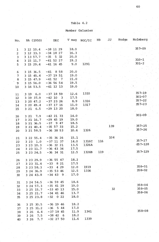
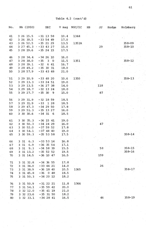
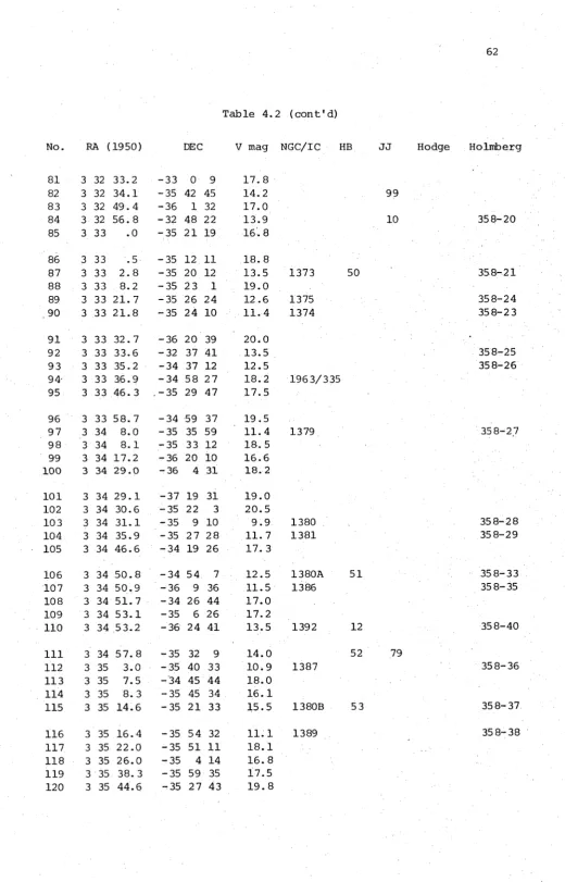
T a b l e 4 . 2 M e m b e r g a l a x i e s 60
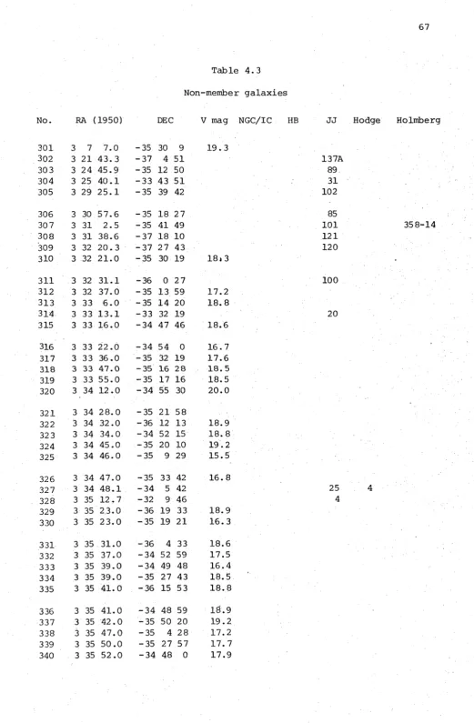
T a b l e 4 . 3 N o n - m e m b e r g a l a x i e s 67
T a b l e 4 . 4 R a d i a l s u r f a c e d e n s i t y 69
T a b l e 4 . 5 E x t r a p o l a t e d t o t a l n u m b e r o f g a l a x i e s 70.
T a b l e 4 . 6 G a l a x y c l a s s i f i c a t i o n s t a t i s t i c s 70
T a b l e 5 . 1 F i t s o f K i n g m o d e l s t o F o r n a x I g a l a x i e s 90
T a b l e 5 . 2 F i t s o f K i n g m o d e l s t o V i r g o g a l a x i e s 91
T a b l e 5 . 3 F i t s o f K i n g m o d e l s to g a l a x i e s i n O e m l e r ' s l i s t 92
T a b l e 5 . 4 F i t s o f K i n g m o d e l s t o l o c a l d w a r f e l l i p t i c a l s 93
T a b l e 5 . 5 D i f f e r e n c e s in f i t s o f K i n g m o d e l s 93
T a b l e 6 . 1 M a g n i t u d e s a n d c o l o u r s - m e m b e r s 1 0 9
T a b l e 6 . 2 M a g n i t u d e s a n d c o l o u r s - n o n - m e m b e r s 1 1 0
T a b l e 7 . 1 D a t a f o r 8 b r i g h t V i r g o e l l i p t i c a l g a l a x i e s 117
T a b l e 8 . 1 L u m i n o s i t y f u n c t i o n f o r F o r n a x I g a l a x i e s 1 2 4
T a b l e C . l C h a r a c t e r i s t i c s o f t h e A A T 163
T a b l e C. 2 V i g n e t t i n g p r o f i l e r e p r e s e n t e d b y s t r a i g h t
l i n e s e g m e n t s 1 6 4
T a b l e C . 3 C h a r a c t e r i s t i c s o f 40" 165
Fig. 3.3 AV as a function of aperture size 41 Fig. 3.4 AU as a function of aperture size 42 Fig. 3.5 Comparison with Hodge's profile of NGC 1399 43 Fig. 3.6 Comparison with Miller & Prendergast's profile
of NGC 3379 44
Fig. 4.1 Galaxy 117, a dwarf in Fornax I ' 7 1
Fig. 4.2 Galaxy 326, a distant galaxy 72
Fig. 4.3 AAT spectra of galaxies 73
Fig. 4.4 Sky distribution of galaxies 74
Fig. 4.5 Distribution of bright & faint galaxies 75 Fig. 4.6 (a) Colour-magnitude array for members 76 (b) Colour-magnitude array for non-members 76
Fig. 4.7 RA marginal distribution 77
Fig. 4.8 Dec marginal distribution 77
Fig. 4.9 Radial surface density distribution 78
Fig. 4.10 Morphological triangle 79
Fig. 5.1 Comparison of fits of King models to Fornax I
Galaxies 94
Fig. 5.2 Comparison of fits of King models to Virgo
Galaxies 95
Fig. 5.3 Log (6) as a function of absolute magnitude for
Fornax I galaxies 96
Fig. 5.4 Lo g (8) as a function of absolute magnitude for
galaxies and globular clusters 97
Fig. 5.7
Fig. 5.8
Fig. 5.9
Fig. 6.1 Fig. 6.2
Fig. 7.1
Fig. 7.2
Fig. 7.3
Fig. 8.1 Fig. 8.2 Fig. 8.3 Fig. 8.4
Fig. A.1 Fig. A.2 Fig. A.3 Fig. A.4 Fig. A.5 Fig. A.6 Fig. A.7 Fig. A.8
for galaxies
Core radius as a function of absolute magnitude for galaxies and globular clusters
I as a function of absolute magnitude for Fornax I galaxies
I as a function of absolute magnitude for galaxies and globular clusters
Colour-magnitude array for Fornax I galaxies Colour-magnitude array for galaxies and globular
clusters
Colour-profile shape relationship for Fornax I galaxies
(a) Colour-magnitude array for 8 Virgo elliptical galaxies
(b) Colour-magnitude array for 8 Virgo elliptical galaxies after removal of colour-profile shape relationship
Colour-profile shape relationship for Virgo galaxies
V^ as a function of photographic magnitude Differential luminosity function
Cumulative luminosity function
Comparison of luminosity function with Schechter function
AV as a function of aperture size AU as a function of aperture size Profile of NGC 1399
Colour-surface brightness plot for NGC 1389 Colour-surface brightness plot for NGC 3115 Axial ratios of NGC 3115
Metallicity as a function of radius
Theoretical colour gradients from Larson's model
cage from the (+) position 169 Fig. C.5 Sky baffle, mirror, and shadow of prime focus
cage from the (-) position 170
Fig. C.6 AAT Vignetting profile 171
Fig. C.7 AAT Vignetting profile with doublet 172
Fig. C.8 (a) Sky values as a function of radius 173 (b) Average sky values as a function of radius 173
Fig. C.9 Diagram of 40" Telescope 174
Fig. C.10 40" Vignetting profile 175
Fig. D.l Four adjacent data points 184
Fig. D.2 Coordinate system for program VIG 184
C H A P T E R 1
INTRODUCTION
Observations of early-type galaxies provide important
constraints on theories of galaxy formation and evolution. Galaxies are thought to have formed by the collapse of primordial material under self-gravity. As the infall proceeds, stars form, evolve and enrich the insterstellar medium with metal-rich material from which the new stars are formed. It is plausible that this enrichment process will be mass-dependent since a massive galaxy has a deeper potential well, is able to attract more material and therefore undergo a greater degree of enrichment, than a less massive galaxy. Observations of the colour- magnitude effect have been limited to bright galaxies and a study of
elliptical galaxies over a wide brightness range would assist in determining the overall behaviour of this relationship.
If galaxies form as subcondensations within the proto-cluster material, the present luminosity (mass) spectrum will reflect the original spectrum, but may, of course, be altered as a result of breakup, collision, merger etc. Observations of the luminosity function of the galaxies within a cluster to faint total brightness will provide useful information which may be effective in arbitrating between competing theories of galaxy formation and evolution. In this way the physics of the breakup of the proto-cluster material may
eventually be understood.
Observatory.
C H A P T E R 2
SYSTEMATIC PROPERTIES OF EARLY-TYPE GALAXIES
This thesis is concerned with the systematic properties of
early-type galaxies in the Fornax I cluster. This includes properties of the individual galaxies i.e. luminosity distributions, to the distribution of galaxies in the cluster. To determine the current understanding of problems associated with early-type galaxies, a literature survey was carried out with the emphasis on the observational results and the-inter pretation of these results in terms of current theories of galaxy forma tion and evolution.
Galaxian luminosity distributions
Observations of a galaxy in a single waveband enable the deter mination of the radial luminosity distribution which is necessary for an assessment of the mass distribution in the galaxy. This provides a basis for the construction of mass models and the start of the understanding of the dynamics of galaxy evolution. The radial luminosity distributions have been quantified by various fitting formulae, which, with one exception,
are purely empirical; the one based on a mathematical theory has severe restrictions in its formulation and its relationship to a real galaxy may be tenuous. All the fitting formulae considered have free parameters which can be adjusted to fit a given galaxy, and are therefore useful for
comparing one galaxy with another.
Hubble (1930) showed that profiles of elliptical galaxies could be conveniently described by
r 2 I (r) - I_/(l + -)
it provides good agreement with observations over a wide range of radius, it has some deficiencies.
de Vaucouleurs (1956) suggested the expression 1/4 log (— ) = -3.33 (— ) " 1
where Ig is the intensity at r = rg , the radius containing half the total galaxy luminosity. This expression converges to a finite total luminosity and provides good agreement with observations over a wide range of radius.
King (1966) constructed a series of models to fit globular cluster profiles, based on the assumption of a single mass for all objects,
isotropic velocity distributions, and an isolated self-gravitating system. He further assumed a Maxwellian distribution function for the stellar kinetic energies and used a cutoff at the high energy end. Each of these assumptions has potential difficulties when relating theory to reality, as King himself emphasises (1978). Nevertheless his models can be used to compare profiles of galaxies with each other, and profiles of galaxies with profiles of globular clusters.
Oemler (1976) modified the Hubble profile with an exponential cutoff at the bright end and demonstrated good fits to profiles over a wide range of radius. His formula was
2
exp(-
(V
/(1 + e>
where a and 3 are scale factors.type of curve covers all types, a point emphasised by King (1978). Lenticular and spiral galaxies have a spheroidal component obeying the luminosity law applying to elliptical galaxies, and a disk component with an exponential fall-off with radius de Vaucouleurs (L958), Tsikoudi (1977).
Galaxy colours
Observations in two wavebands give colour information which is central to analysis of the age and chemical evolution of the galaxy. Differences in colour from one part of a galaxy to another have been observed and can be related to theories of galaxy formation and ' evolution. In this review we discuss the evidence for changes in the integrated colour from one galaxy to another, and then note the
evidence for colour changes within individual galaxies.
Colour-magnitude array
The significant observations of the integrated colours of early-type galaxies have resulted in the relationship between colour and absolute magnitude. The nature of this relationship has been known for some time but has only recently been thoroughly documented. The explanation of the effect is not well understood, although there are good grounds for believing that metallicity changes are responsible.
Baum (1959), de Vaucouleurs (1961), Rood (1969), and Sandage (1972) have produced observational evidence demonstrating the relation ship between colour and absolute magnitude. The study which has
A(u-V)/a v = 0 . 1
The significance of the VS work is in the demonstration of a linear relationship between colour and magnitude for bright early-type galaxies. This was based on a composite CM array and VS claimed
#
universality for this result. What is true is that the early-type galaxies followed, in the mean, the overall relationship. However, it does not necessarily follow that each cluster separately has'the same slope as the composite array. The number of galaxies observed by VS in the separate clusters is too small to make detailed comment on differences between the various clusters.
The VS sample consists mainly of galaxies brighter than
M^ = -18.7, but includes 5 dwarfs in Virgo measured by Sandage (1972). These dwarfs are important since they are the only available observa
tions fainter than M = -18.7 and have therefore been accorded a high v
statistical weight in the definition of the mean CM relationship. One aspect of the CM work discussed by Baum (1959) and by
some 9 magnitudes between the faintest of the well observed VS galaxies and the brightest of the globular clusters.
Faber (1973) made a significant advance in the attempt to understand the physics of the CM array, using 10 carefully chosen intermediate-band filters to examine colours and metal line strengths of close pairs of elliptical galaxies. She found intrinsic colour and metal line strengths showed monotonic relationships with total magnitude, and concluded that the observed colours were consistent with the
hypothesis that variations in colour could be accounted for by variations in metal abundance alone. This was an important step as it was the
first comprehensive evidence that a single parameter, metal abundance, varied with total mass.
Further evidence that metallicity varies systematically with absolute magnitude and is enhanced in galaxy cores comes from Cohen
(1979). She measured the equivalent widths of several absorption features on the red side of 5000$ and found that those features which showed radial variations within galaxies also varied from galaxy to galaxy. Those features that showed no radial variations within the galaxies did not vary from nucleus to nucleus. Cohen postulated that these observations were consistent with the hypothesis that a single factor caused both the radial variations within the galaxies and the variations from nucleus to nucleus between the galaxies. This single factor she identified as metallicity.
Kalinowski (1974), Miller and Prendergast (1962), (1968), Strom et al., (1976), Strom et al., (1977), Strom et al., (1978), Duus (1978) (Appendix A ) , and others. These results influence theories of galaxy formation and evolution since at least three interpretations of radial colour changes are possible. Many early-type galaxies have cores which are redder than the outer parts which may mean (a) increasing interstellar absorption near the galaxy center, or (b) metal-rich stars near the center with a declining gradient as a function of radius, or (c) age differences with the younger bluer stars near the periphery, or a combination of these interpretations.
Luminosity function
The luminosity function of a cluster of galaxies describes the distribution of absolute magnitudes of the members of that cluster. If the mass to light ratio is known independently, the luminosity function can then be interpreted in terms of the mass spectrum of the galaxies in the cluster. This should assist in understanding the
physics of galaxy formation in the protocluster, since the present mass distribution is derived from the original distribution, though the processes of galaxy merger and breakup may have modified the original distribution.
Luminosity functions have been published by Kiang (1961),
He constructed two functions; for the first, the background was constant over the area of the cluster considered, which he considered was an
overestimate of the true correction; in the second, he assumed no
background galaxies were present, which was certainly an undercorrection. He compared his results with a similar determination by Abell and found reasonable agreement. Interestingly, both Rood and Abell found the luminosity function was not monotonic increasing, but that dips were present at approximately the same brightness in both samples.
Oemler (1974) measured the luminosity function for 15 clusters, with the data obtained in a consistent fashion for each cluster. His result for Coma shows some resemblance to Rood's, discussed above, but examination of his Fig. 4 reveals a wide variety of profiles for differ ent clusters. The background problem is severe in Oemler's work, since he used as a background correction, the average background determined over all the clusters.
Oemler's results have been used by Schechter (1976) who formed a composite luminosity function of 13 clusters. The method used to combine the clusters has resulted in the final profile representing a mean of all the clusters involved, irrespective of the richness of the individual clusters. In this way, the final function is dominated by the richer clusters. Schechter formed a function of the form
n (L) dL = n* (^*)a exp(- jr*) d (^)
where the important power term is given by a = -1.24 and the scaling factor n* = 910. The Schechter expression has been used by
Dressier (1976) and Jones and Jones (1979) in recent studies of the luminosity function.
spectrum at the bright end at formation time was governed by random events, or that the original spectrum has been entirely obliterated by breakups, mergers, collisions etc. Dressier's clusters were
necessarily distant objects, and his luminosity profiles are determined to ^ -19.5. Therefore no information could be obtained on the shape of the luminosity function at fainter magnitudes.
Turner and Gott (1976) formed a composite luminosity function from a selection of small groups of galaxies. Their method of combining the clusters avoided the problem of domination of the poorer clusters by the richer clusters (eg. Virgo), however the main difficulty with their work is the method used to define the groups that • make up the catalog. They identified regions of the north galactic cap which showed enhancements in the surface number density of galaxies brighter than V ^ 14.0. By
adopting a precise objective criterion for selection of galaxies into a group, they ensured that all recognised clusters were included, but made it difficult to distinguish open clusters from a chance alignment of field galaxies. The problem of correct background identification is therefore greater than the problem of identification of the members of individual groups. Despite these difficulties, their work is the first attempt at construction of a luminosity function for small groups, and they found good agreement with the Schechter shape with a = -1. Their result is essentially a bright galaxy result, because the sample was limited to galaxies brighter than V 14.0.
Jones and Jones (1979) undertook a program of velocity deter mination for galaxies in the magnitude range 15 < mn < 16 in the Schmidt
field 358 which covers the Fornax I cluster. The theoretical ideas behind their program are described in Jones and Jones (1978), where they show that if the field galaxies have the same luminosity function as the cluster under consideration, it is possible to differentiate between two extreme luminosity functions and thereby obtain informa
tion on the faint end of the luminosity function. The two luminosity
functions chosen were a Schechter function (1976) and a Schechter
function with an exponential cutoff at the faint end. Their aim was
to be achieved by determining membership for a complete sample of
galaxies in a specified narrow range of apparent brightness. The
observations should adequately cover the extent of the cluster and
include a large sample to get meaningful results. The problem with
this scheme is in the assumption that the cluster and field have
identical luminosity functions. Of course there is no way of telling,
a priori whether the functions for the cluster and the field will be the same, and it would be important for that hypothesis to be examined.
In the course of their radial velocity determinations, they
accumulated sufficient redshifts of galaxies down to = 16 to
construct the luminosity function for the part of the Fornax I cluster
covered by field 358. Comparison with the Schechter function gives a
best fit with a = 0, significantly different from the earlier results of Schechter and Dressier.
Stellar populations in early-type galaxies
The stellar content of galaxies has been the subject of a large amount of investigation, in particular Morgan (1958), King (1971),
and van den Bergh (1975). Elliptical galaxies, in particular, are
reflected in the integrated colours of these systems.
The Bright End of the Luminosity Function
One aspect of the luminosity function work which has aroused much interest is the distribution of the absolute magnitudes of the brightest galaxies in clusters. The particular question that is to be answered is - 'is the brightest galaxy in a cluster formed by a process different from that which forms the other cluster members, or is
galaxy formation a statistical process with the brightest galaxy formed at the bright end of this process?"
Sandage and Hardy (1973) and Sandage (1976) favour the special process interpretation. Sandage argues that the observed luminosity
functions are not steep enough at the bright end to fit the observa tional results and therefore no universal luminosity function applies. He sees the brightest galaxy in a cluster formed by a process which is different from the formation processes for the other cluster members.
The opposing view, that luminosity functions are universal and the brightest cluster galaxy is part of the same statistical formation process, has been surveyed and summarised by Geller and Peebles (1973). They note the small dispersion in the absolute magnitudes of the
brightest galaxies in clusters and the homogeneoty of form of luminosity functions as major points in their argument.
the most massive galaxy. This galaxy could grow at the expense of other members of the cluster and the present luminosity function could bear little relationship to the original luminosity function.
HI content of early-type galaxies
Observations of the HI content of early-type galaxies are important as theories of galaxy formation and evolution make specific predictions about the fate of expelled and remaining primordial gas within the cluster. These observations have detected very small amounts of HI in some ellipticals and very low upper limits in others.
Bottinelli and Gougenheim (1979) and references therein discuss the latest results. Further discussion is left to the section on theories of galaxy formation and evolution.
Classification of Clusters
The purpose of a classification scheme for clusters of galaxies is to identify the major types of cluster by some gross, obvious
Eggen, Lynden-Bell, and Sandage (1962). The globular clusters are thought to have formed early in the life of the collapsing protogalaxy, dwarf galaxies are thought to have formed far from the parent galaxy, from material not partaking in the initial collapse. As a result, some
similarity can be expected between the modes of formation of the globular clusters and the dwarf galaxies. It may also be expected that this
similarity would be reflected in the present structure and properties of these objects.
The globular clusters seen around our galaxy have, on passing through the galactic disk, encountered the potential field of the disk and have, in the main, survived its disruptive effect. They have survived because the gravitational fields caused by the high stellar densities
near their centres dominate the field of the disk.
The dwarf elliptical galaxies on the other hand are less compact, more diffuse objects and couldn't survive a close encounter with the Galaxy. It is likely therefore that the dwarfs formed further away from the Galaxy than did the globular clusters, and that the dwarfs seen today have never come close to the Galaxy. Hodge (1966) discusses this point with respect to the 6 better known local dwarfs.
Evidence relating the King structural parameter log (r,/r ) for t c elliptical galaxies, dwarf ellipticals, and globular clusters has been discussed by King (1962) and Freeman (1975), who note the similarities
in this parameter for these three classes of object.
array and variable star content has come from Baade and Swope (1961), (who studied the dwarf elliptical Draco), Hodge (1965) (Sculptor), van Agt (1967) (Ursa Minor), and Swope (1967) (Leo II). Baade and Swope note the basic similarities in the colour-magnitude array and in the luminosity function between Draco and the globular clusters, while van Agt finds similar colour-magnitude arrays for Ursa Minor and
comparison globular clusters. van den Bergh (1975) lists the differ ences found between dwarf ellipticals and globular clusters in comparison of certain classes of variable stars.
Observations of colour and line strengths of elliptical galaxies and globular clusters by Faber (1973), McClure and van den Bergh (1968), and Aaronson et al., (1978), have emphasised the similarity between the 2 types of object. As noted above, Aaronson et al., used infrared colour observations to calibrate mass dependent metallicity changes.
Theory
The observational results discussed above are now used in
discussion of theories of galaxy formation and evolution. In particular, we discuss models of the mass distribution in clusters, several theories of galaxy formation and evolution, and the fate of interstellar gas within the cluster.
Mass models of clusters
Peebles (1970) modelled the Coma cluster and produced a creditable comparison with the observed mass distribution in that cluster. White
(1976) also modelled the Coma cluster and found good agreement with Oemler's (1974) mass distribution.
Butcher and Oemler (1978) have provided a series of curves representing Aarseth's models of projected mass density as a function of radius with which observational results can be compared. The
parameter defining the curves is a concentration index log (R^Q)/log (I^q). where is the radius containing n percent of the projected mass. Thus it is relatively simple to relate actual distributions to the
theoretical predictions and hence, via the (unpublished) details of the models, to the various initial conditions.
It should be noted that interpretation of observational results in terms of theoretical models may not be satisfactory and that compari son with different theoretical models may not lead to consistent
conclusions. This problem has been highlighted by the work of Lecar (1968) who organized 11 investigators to model and integrate the
However the comparisons between models with various values of should not be affected and therefore clusters can be compared on the basis of their various R values.
n
Theories of galaxy formation and evolution
Gott (1973) proposed a theory of galaxy formation in which the protogalaxy consisted of stars without any remaining primordial gas, and which came into virial equilibrium to form an elliptical galaxy. The elongation of the resulting galaxy was directly related to the initial angular momentum of the system, and the galaxy has smooth isophotes similar to those observed in elliptical galaxies. As no primordial gas remains in the protogalaxy before its collapse, there is no star formation after the collapse has started, and therefore all stars will be of the same age. This theory therefore excludes metal enhancement and consequently predicts no colour variation across an early-type galaxy. This prediction is not in accordance with observa tions (see earlier discussion of observed colour gradients), and there fore casts doubt on the validity of Gott's theory.
Larson (1975) detailed a series of models in which primordial gas, constituting the protogalactic material, collapsed under selfgravity and formed stars with the timescale for dynamical collapse equal to the timescale for star formation. The remaining gas cools and sinks toward the galaxy center with a cooling timescale equal to the dynamical
observed colour gradients in early-type galaxies will be different along major and minor axes, after allowance for the elongation. This prediction, often conveniently expressed as "isochromes flatter than isophotes", was claimed by Strom et al., (1976) and Strom et al.,
(1977) to have been observed in NGC 3115. Their published data was examined by Duus (1978, Appendix A) who used a more sensitive method of data analysis and has showed that the effect as predicted by Larson was not present in their data. The flattening of the isochromes was not present in NGC 1389, an elongated galaxy in Fornax I chosen to investigate Larson's prediction. Furthermore, the shape of the colour-surface brightness plot bears little relationship to the prediction made by Larson.
Second, Larson's models are supported by rotation, i.e., the elongation is a result of the rotation of the galaxy. Illingworth
(1977), and Schechter and Gunn (1979) and references therein have
shown that the observed rotation is not in accord with this prediction, but is approximately 1/3 that predicted by a model supported by
rotation.
A third difficulty concerns the fate of the expelled inter stellar gas. The metal enrichment theories, of which Larson's is the prototype, require the presence of interstellar gas, which can be a mixture of both primordial and processed gas, to act as the raw material for the enrichment process. The theoretical amounts of HI
galaxy obtained. Observations of HI in early-type galaxies have placed very low upper limits ( < 0.1% by mass) on the HI content. Therefore the predicted amount of gas is either present in the galaxy and has not been observed or has been swept out of the galaxy by some undetermined process.
Galactic winds
This idea was first investigated by Mathews and Baker (1971) and Larson (1974) incorporated it into his models. Essentially the process can be described as follows - gas injected into the interstellar medium with the velocity of its parent star, and therefore high
relative velocities are present between the various gasses. At the fronts, shocks will keep the gas hot and prevent it cooling by radia tion. Supernovae explosions now play their part by sweeping up the hot gas and driving it out of the galaxy. Mathews and Baker considered a steady-state outflow would be established and no observable gas would remain.
In pursuing this idea, Faber and Jackson (1976) noted that the velocity dispersion in galaxy centers was related to total brightness by
4
L a v
where L is total brightness and v is the velocity dispersion. If this relationship holds throughout the galaxy, the kinetic temperature of the expelled gas will be greatest in the most massive galaxies. In less massive galaxies, this gas would cool and condense between
no galactic wind could operate.
Given these uncertainties in the model, it is difficult to assess the importance of the galactic wind, except to note that Faber's (1973) data gives some hope for the theory expounded by Faber and Jackson. If no gas were expelled from the galaxy, it is reasonable to imagine that star formation would continue up to the present epoch. This in turn would result in the colours of apparently early-type galaxies becoming
significantly bluer than the trend seen in the CM array, below a certain brightness level. This effect is seen in Faber's data at M^ -16.5 where 3 galaxies are considerably bluer than would be expected by simple
extrapolation of the mean CM line.
Previous observations of the Fornax I cluster
Appendix B summarises previous observations of the Fornax I cluster. These observations cover many of the facets discussed above, and are referred to at appropriate places within the thesis. In particu lar, several important parameters are mentioned in Appendix B and are used in subsequent analysis.
These are
-(a) Fornax I has a galactic latitude of -55°, and I assume galactic reddening and absorption are zero at this latitude;
i) Photography
The Fornax I cluster was divided into 4 overlapping 1° fields numbered 1-4. Fig. 3.1 shows the centers and the 1° square field of the Anglo-Australian Telescope (hereinafter AAT). The corresponding field on the 40" was circular, with the same center and diameter of 1°. It was intended originally that all 4 fields would be covered in the U and V wavebands; however restrictions on observing time limited the project to fields 1 and 2.
The choice of the most appropriate wavebands for these observa tions was decided by referring to VS Fig. 1. This graph shows the luminosity distribution as a function of wavelength for Virgo galaxies
c
with 8.7 < V 0 _ < 14.0. The curves have been shifted vertically to 26
coincide at 6213 A ° . The greatest difference in the curves occurs at the shorter wavelengths; therefore the U and V bands were chosen to best exhibit this difference.
The photographic bandpasses were defined by the following (plate, filter) combinations; U, IlaO plus UGl ; V, IlaD plus GG14. A journal of the photographic observations is given in Table 3.1.
The AAT was used for the U and deep V exposures. The AAT has 2 prime focus correctors - the doublet and the triplet, each giving a platescale of 16.24"/mm. The latter is unsuitable for use in the ultraviolet as it is constructed of UBK7 (AAT User's guide) and has one of its surfaces coated with antireflective coating to reduce ghosting produced by internal reflection. This coating has had its
and has a steeply decreasing transmission below 4000^P. Therefore the observer is forced to use the doublet for ultraviolet observations.
There is, however, a serious drawback with the doublet, which is not satisfactorily described in the AAT User's guide. The design and size of the doublet, together with the geometrical alignment of the
asymmetrical prime focus cage and the camera, have resulted in two sources of vignetting.
The first source, resulting from the design and size of the doublet, causes a marked decrease in sky brightness outside a central 25' diameter field. This vignetting has been calculated by a ray-tracing procedure described in Appendix C. The essential optical elements of the AAT and corrector are listed in Table C-l and used in conjunction with established methods of ray tracing to determine sky brightness as a function of distance from the centre of the field. Appendix C lists details of the procedures used together with results of sky measurements
from the plates.
The second source of vignetting on the AAT results from the geometry of the asymmetrical prime focus cage, the primary mirror, the sky baffle, and the position of the prime focus camera in the cage. At any point in the prime focus plane, the level of sky background depends on an azimuthal term which is a function of the relative positions of the camera and the cage. Since there was no facility for recording this information when these observations were made, it was not possible to correct for this effect.
The A.N.U. 40" telescope was used for the short V exposures. There is an f/8 secondary and a plate scale of 25.2"/mm at the
(a) Calibration
The full calibration procedure consists of 2 separate procedures: (1) sensitometry - the conversion of measured densities into intensities, and
(2) standardization - the determination of the relationship between the intensity scale from (i) and the standard UBV photoelectric system.
(1) Sensitometry
The usual method of converting a density scale into an intensity scale is to use a sensitometer in which a pattern of spots of known relative intensity is projected onto the plate. A calibration curve is constructed by plotting the measured densities of each spot against the known relative intensity of the light that produced the spot.
A tube sensitometer, housed in the 40" building, was used to provide calibration spots in conjunction with plates taken on the 40" telescope. This particular sensitometer used either a tungsten or a quartz lamp, and an opal diffuser which provided uniform illumination on the entrance holes. These holes, which were of varying sizes, were connected by tubes to the exit holes which were of constant size,
(hereinafter EBN) and which were used in this project.
There is a choice of lamps available for use with the 40" sensitometer - a tungsten lamp for use in the B and V wavebands, and a quartz-iodine lamp for the U: there is provision for filters to be placed in the light path.
There were several problems associated with the use of the spot sensitometer. First, the opal diffusion had a transmittance with an unknown wavelength dependence and the effective wavelength in either of the U or V wavebands may have differed from that defined by the photo electric system. Second, the sensitometer was housed in a room away from the telescope and it was not possible to guarantee that the same conditions of temperature and humidity applied to both. Therefore it was decided to use photoelectric photometry to effect minor changes to the calibration curve to ensure agreement between photoelectric and photographic results.
(2) Standarization
The intensity scales defined by the calibration curve were matched to the standard UBV system by photoelectric photometry, as described below.
(ii) Photoelectric Observations
Two types of photoelectric observations were undertaken -(a) repeated centred aperture measurements, and
(b) drift scans across NGC 1399 to check the slope of the V calibration curve.
(a) Repeated centred aperture observations
is also shown, assuming a scale of 11.3"/mm. To ensure the best possi bility of the photocell, a standard procedure of filling the ice box every 6 hours, day and night, during the entire observing run, was adopted. At the commencement of the observing run the most sensitive part of the IP21 cathode was located by observing a bright star and moving the cell laterally until the count rate showed a maximum. The cell was then firmly fixed and all observations carried out with the cell in that position.
Standard stars were chosen from Cousins' (1973) E regions, El and E2. These 2 regions straddle the Fornax I cluster in Right Ascension, and the particular region chosen was determined by conditions at the time of observation. The standards were observed in groups of 5 or 6 at intervals of 90 minutes during the night.
The integration times for stars were 10 seconds in each filter, but the times for the galaxies varied between 20 seconds in V to 60 in U. Sky measurements were made between each galaxy measurement and a nett 10,000 counts achieved.
Each galaxy was centered at the beginning of a series of obser vations by moving the aperture in small steps in RA and Dec across the galaxy and finding the position which gave the maximum count rate. This position was then adopted for all observations of that galaxy. Sky
measurements were made between each galaxy measurement at positions chosen from deep plates to be free of any contamination.
observations and reduction. A BASIC program was used to record the counts in each integration period, interrogate the RA and Dec encoders, and input the siderial time. All stars and galaxies were observed in
the sequence UBWBU; the airmass was calculated at the midpoint of
that sequence.
Standard values of extinction in the V, U-B, and B-V systems
were assumed and are shown in Table 3.4. From the natural magnitudes
and colours, AV(natural-published), A(B-V) and A(U-B) were plotted against V, (B-V), and (U-B) respectively to define the transfer
equations. These were calculated for each set of 5 or 6 standard stars,
and used to reduce the program galaxies observed in the intervening periods.
Repeated observations of the same standard stars over several nights enabled an estimate of the accuracy of the observations to be
made. Using the appropriate transfer equations, the derived values
V, (U-B), and (B-V) could be determined for the standard stars and compared with the published values. The average standard deviations over all standards was then found for V, (U-B), and (B-V) and are shown in Table 3.5.
For the 4 program galaxies, observations were averaged and a
mean and standard error calculated: these appear in Table 3.6. The
corresponding standard deviation per measurement is approximately 0.03 magnitudes.
(b) Drift Scans
The drift scans were done on the 40" using the GPS data system
and a program written by Dr Ken Freeman. In this section we discuss the
the aperture in the manner described earlier, the telescope driven off to the west and a suitably bright star chosen as the reference point. The telescope was advanced slightly further to the west, the tracking disabled, and the integrations commenced as the bright star crossed the vertical cross hair. At the end of each scan a plot of the data was displayed on the Tektronix screen and the observer had the option of accepting or rejecting the scan. If accepted, the scan was co-added to the previous scans and the current mean scan displayed on the screen. The total integration time was 360 seconds per scan and a total 9 scans were used to give the final scan which was then recorded on cassette for later processing.
The reduction program read the data from cassette, allowed the operator a large degree of control and flexibility in the removal of unwanted stars, and produced a final "clean" scan. The star removal procedure required the operator to define, by the use of cursors, the part of the scan defining the galaxy and from which no stars were to be removed. In the region external to this, a cleaning procedure was used which involved successive passes through the data replacing points more than 3 standard deviations above or below the mean, with the mean value. After no more points had been rejected, the level for rejection was
(iii) Microphotometry
The PDS microdensitometer at the Anglo-Australian Observatory was used to scan the photographic plates. The PDS consists of a light
source and an optic train which projects an aperture (called a pre-slit) onto the photographic plate. This projected aperture is examined by the optics of the upper stage (the scanning slit) which uses a photo multiplier tube to record the amount of light transmitted through the
plate. The basic quantity measured is the transmission, T, defined
m 1 out
T = ---I .
m
This transmission can then be converted to density by a Log
converter. Density (D) is defined
D = log (~)
The setr up and operating procedure recommended in the PDS operations
manual were followed with several modifications. The purpose of the
adopted procedure was to ensure that the PDS measuring runs were as similar as possible to each other, and that the setup sequence was
simple, methodical and easily remembered. The features of the adopted
procedure were
-(a) the use of a piece of clear glass, of the same thickness as the exposed plate, as the standard for setting the PDS voltage and density controls;
(b) the use of opaque material to set the zero for measurements in transmission mode;
(c) the use of maximum gain during transmission measurements; (d) the use of an offset of 020 (density 0.2) during density
measurements;
deep V plates were scanned with a 20 micron square aperture. The. brighter
galaxies on the U and deep V plates were scanned with either a 50 micron
or 125 micron square aperture. To achieve this range in aperture size,
use was made of the * 4 and * 10 objectives in the PDS optical train.
As the density mode gives a better resolution than transmission
mode at higher densities, the mode selected for a particular measurement
depended on the part of the galaxy under investigation. Central parts
of the bright galaxies on the short V exposures were scanned in density
mode, whilst the faint galaxies and outer parts of bright galaxies were
scanned in transmission mode.
Each line was scanned with the step size, the distance between
sample points, equal to the aperture size. Adjacent scan lines were
made in opposing directions, with a separation equal to 1 aperture size.
All galaxies were scanned in a square array with the number of scan
lines equal to the number of measurements in each scan line.
Transmission scans were done at the maximum speed available
(255 PDS speed units). Density scans required a little care as the
L o g amplifier had a finite time constant which meant it was unable to
expand instantaneously to rapid changes in input signal. Herzog and
Illingworth (1977) found speed restrictions were necessary to guarantee
accurate measurements of stellar images. Trial scans across galaxy
centres were made at varying speeds, but no speed-dependent effect was
found. Nevertheless, all density scans were carried out at 16mm/sec
(iv) Calibration Curve
The Sensitometer produced a pattern of 3 rows of 5 spots. These spots and the areas of plate between the spots were scanned with the PDS and the density of the spots above fog determined. The calibration curve was then constructed, using the geometrical measures of the diameters of the sensitometer entrance holes as the gauge of the relative intensity of the light passing through the holes.
The form of the calibration curve used is that described by de Vaucouleurs (1968) which is in turn an adaption of an earlier system described by Baker (1925). The abscissa is in units of log (intensity) and the ordinate in terms of log (w) whereas u) = 10D-1. The effect of this formulation is to straighten out the calibration curve particularly at the faint end, and thereby allow representation by a polynomial.
A polynomial of the third order was fitted to the points in the (log (w), log (I)) plane. The various aperture sizes on the PDS were obtained with the *10 and x4 objectives which "see" the plate at differ ent effective f ratios, and the measure of density through each varies slightly over the range of densities encountered. Therefore separate calibration curves were required for each objective/plate thickness/ emulsion type combination and the coefficients of the polynomials representing these calibration curves are listed in Table 3.7.
The calibration curve in the V band was adjusted by comparison with the results of the drift scans. Fig. 3.2 shows the final agreement.
The calibration curve in the U band was adjusted by comparison with centred aperture observations published by VS.
(v) Data Reduction
[image:44.554.20.535.29.812.2]of similar concentric ellipses with major axes colinear. Appendix E contains details of this model.
(vi) Internal checks on the photometry
The orientation of fields numbered 1 and 2 were deliberately chosen to give an area of sky common to both fields. There were 8 faint galaxies in this overlap region in the magnitude range
16.5 < V < 19.8. Since this number of galaxies was not sufficiently large to support a complete error analysis as a function of magnitude, the mean magnitude, V = 17.7, was adopted to represent the sample.
The standard deviation of the differences in the V magnitudes from centre 1 to centre 2 was 0.13. The corresponding error for the U magnitudes was 0.16, giving a total internal error of 0.21 in (U-V) at V = 17.7.
(vii) External Checks
(a) Comparison of Photographic Magnitudes with Photoelectric Magnitudes
The repeated centred aperture photoelectric observations in the V waveband described in (ii) above were used to set the zeropoint of the V magnitude scale. The drift scans in the V waveband also described in
(ii), were used to set the shape of the V calibration curve.
from Hodge (1963); the others are from Sandage (1975) and Sandage and
Visvanathan (1978). The galaxy observed by Hodge and by Sandage and
Visvanathan through small apertures is NGC 1399; the differences in
observed magnitudes demonstrate the problems associated with small
aperture observations of galaxies. For the remaining observations, the
standard derivation in AV is 0.042 magnitudes. Using a standard
derivation for photoelectric measurement of 0.03 magnitudes ( (ii) above),
the standard derivation for photographic magnitude is also 0.03.
Repeated centred aperture photoelectric observations in the U
waveband were used to set the zeropoint of the U magnitude scale. The
shape of the calibration curve was determined by use of the sensitometer
and adjusted by comparison with published centred aperture photometry.
The final comparison is shown in Fig. 3.4 with AU as a function of radius
of aperture. The mean difference between photoelectric and photographic
measurements is -0.028 with a standard derivation of the differences of
0.053.
(b) Comparison of Photographic Galaxy Profiles with Published Profiles
A check on external consistency can be achieved by comparing
photographic galaxy profiles with those determined by other observers.
This gives a check on the entire range of the calibration curve, as
distinct from the centered aperture comparison which generally include
only the brighter sections of the galaxy.
Hodge (1978) published an E-W profile of NGC 1399 which is
compared to the results of this study in Fig. 3.5. As noted in Fig. 3.3
there is a zero point difference between Hodge's photoelectric observa
tions and the results of the current study, and therefore his profile has
s .
C tP •H C
p S
>4-1 (1) o
-I o
rH * 04 X I
aj
r - r* r- r~ £ r - P* r*
3 o o o o
cn cn in in
oö CO CO 00 co o
i
CN
a!
> Q
□ 9 Q Q►4
Q Q
§ §
0 2 2 < 2 < < w u
ß <D x p o s u r T im e c B c •ä c •ä c ■a c £ C B c t c t § § in
CO inCO in 2 o s
w
ä
p
D oD in cn incn
G G 1 4 G G 1 4 G G 1 4 G G 1 4 2 c E m u l s io n * $ w M Il
a
O
*
Q Q Q Q Q
0
«
M
M MM MM M MM <TJ M
<D cn
§ i> l 1 8 H v) 2
E-> 3 Eh s Eh 3 Ö
r r Ör r O Ö■^T
'S ■g 00 00 CO CO
0 a g g g g
c u
2 2 2 2 2 2 2 2
3
o o CN
CN o o o
o
3 cn g g
cn CO m CO CO
in
m mCO inCO mc o inCO inCO CN CN
l i l i i i + +
r - o o in o o o o
0 Wm
c o VOm vOin inCO rH o g g m
CO inCO inCO inCO Pi vO vO X3
c o CO c o c o CO CO o o
M cn
3 a;
U) rH M rH 2 CN u CN 2 rH <D H
3 P •H C
p p p p p
c
p O a>
U u o Ü 0) u
0) H cn cn
o « = - = - r
c o
CO COCO E
3 O
2 82
0
vO
0) c o in•^r 2 £ mGO vO CO 4J nJ in H
in m in cnCO cn
c o 00
CO COCO
01 »H ■S Eh $H CO CD d 4-1 0 CD •H g 4-1 0 cd 4-1 d •H •H co ft d Q) 0 co U 4-> CD O CO ft CD COft Eh CD ft 4-> • CO ft u 0 CD 4-1 CD CD ft g d •H ?3 •—1 u i—1 •H (D g ft 4-1 ■ft d 01 4-> X CD 0 4-> T3 01 CO d d ■r4 CO CO 01 d ft U •H ft 4-1 U a) 4-1 a) u d to o & w ft }H (d Q a) 4-1 fd 01
a) X 4-1 w
d H
ro 0
+
CM 04 ro
I— I
0 0 H rH 0 2 +
04 tH
O 2
+
ro ro
t— I r—I
0 0 0 0
in 0 2 + I—I I— I 0 2 +
CM rH
ro 0 0 2 2 + +
CM CM
rH rH
0 0 0 0
LO 0 2 + LD 0 2 + rH I— I 0 2 +
i—1 o i—1 i—1 CM CM CM CM CO •H ft V--• •—- -—- -—r ■—- r
d ft X LO ro ro ro ro
o ft 0 0 0 0 0 0
•H CD 2 2 2 2 2 2
4-1 ft 4-1 + + + + + +
cd 4-1 • 43 __ -—- -—. s ^—s -■—
d 2 ft 04 04 04 CM CM CM
■H CO CQ - r l ■— ■ 1— — 1 ■— 1 —
—-ft -H f t f t ro ro ro d 1
|2 ■—1 i—1 rH i—l rH i—1
0 CO rH 0 0 0 0 0 0
U 4-> 43 0 0 0 0 0 0
01 d f t f t 0 u CD 01 •rH cd 4-1 g CO u fd •H rH i—i Eh —
d d CO
g d u ai d
CD •H i—i iH -H CM O O CM O O
\ td d g CM CM 04 CM
U CD a CO ^ i—1 i—1
CD SH o
4-1 d Q) P i 1--1 ft sh f t •rl • r l CD f t f t f t £
T a b l e 3. 3
A p e r t u r e h o l e s i z e s m e a s u r e d b y a Z e i s s m e a s u r i n g m a c h i n e
A p e r t u r e D i a m e t e r i n D i a m e t e r i n s e c o n d s o f
I I
m i c r o n s a r c ( s c a l e = 1 1 . 3
A 395 4 . 46
B 784 8. 86
C 1565 1 7 . 6 8
D 1920 2 1 . 70
E 3166 3 5 . 7 8
F 4 7 8 8 5 4 . 1 0
G 7372 8 3 . 3 0
H 95 72 1 0 8 . 1 6
T a b l e 3 . 4
E x t i n c t i o n c o e f f i c i e n t s
k v = 0 . 1 6
k b _ v = 0 . 1 2 - 0 . 0 4 ( B - V )
k u- b = 0 • 36
Tab l e 3 . 5
A v e r a g e s t a n d a r d d e v i a t i o n s f o r o b s e r v a t i o n s o f s t a n d a r d s t a r s
U-B B-V V