This is a repository copy of Modified flux-vector-based Green element method for problems in steady-state anisotropic media—Generalisation to triangular elements. White Rose Research Online URL for this paper:
http://eprints.whiterose.ac.uk/87814/ Version: Accepted Version
Article:
Lorinczi, P, Harris, SD and Elliott, L (2011) Modified flux-vector-based Green element method for problems in steady-state anisotropic media—Generalisation to triangular elements. Engineering Analysis with Boundary Elements, 35 (3). pp. 495-498. ISSN 0955-7997
https://doi.org/10.1016/j.enganabound.2010.09.004
© 2010, Elsevier. This is an author produced version of a article, published in Engineering Analysis with Boundary Elements. Uploaded in accordance with the publisher's
self-archiving policy. This manuscript version is made available under the CC-BY-NC-ND 4.0 license http://creativecommons.org/licenses/by-nc-nd/4.0/.
[email protected] https://eprints.whiterose.ac.uk/
Reuse
This article is distributed under the terms of the Creative Commons Attribution-NonCommercial-NoDerivs (CC BY-NC-ND) licence. This licence only allows you to download this work and share it with others as long as you credit the authors, but you can’t change the article in any way or use it commercially. More
information and the full terms of the licence here: https://creativecommons.org/licenses/
Takedown
If you consider content in White Rose Research Online to be in breach of UK law, please notify us by
Modified Flux-Vector-Based Green Element Method for
Problems in Steady-State Anisotropic Media - Generalisation
to Triangular Elements
P. Lorinczi
a,∗
, S.D. Harris
b, L. Elliott
caSchool of Earth and Environment, University of Leeds, Leeds, LS2 9JT, UK
bRock Deformation Research Ltd, School of Earth and Environment, University of Leeds, Leeds, LS2 9JT, UK
cDepartment of Applied Mathematics, University of Leeds, Leeds, LS2 9JT, UK
Abstract
This paper is concerned with the generalisation of a numerical technique for solving problems in
steady-state anisotropic media, namely the ’flux-vector-based’ Green element method (‘q-based’ GEM) for anisotropic
media, to triangular elements. The generalisation of the method to triangular elements is based on the same
concepts as for a rectangular grid, namely satisfying a nodal flux condition at each node of the mesh and the
continuity of the tangential pressure gradient across the elements sharing a node.
Key words: Flux-vector-based Green element method, anisotropy, permeability
1
Introduction
Anisotropic media are widely encountered in nature, for example in oil and gas reservoirs. In many
reser-voirs, the production of gas and oil is seriously affected by the highly anisotropic and/or heterogeneous
structure of the media.
Steady-state problems in anisotropic media can be solved using the modified ‘q-based’ GEM for anisotropic
media, introduced by Lorinczi et al. [1]. The approach introduced by Lorinczi et al. [1] has been
im-plemented for non-uniform rectangular grids. Lorinczi et al. [2] used this in geological problems in
faulted/fractured anisotropic media.
A similar approach has been previously introduced by Lorinczi et al. [3] for isotropic media, and it
was applied to highly-heterogeneous isotropic media. The two approaches are using the concept of the
∗
Corresponding author. Tel.: +44-113-3435213
‘q-based’ GEM (Pecher et al. [4]), which maintains the high-order accuracy of the GEM, diminished by
some approximations used in the GEM, see Taigbenu [5].
This paper introduces the ‘q-based’ GEM for anisotropic media for triangular elements. Lorinczi et al.
[3] showed that the q-based’ GEM for isotropic media can be naturally extended to triangular finite
element grids. The work presented in here is based on satisfying similar conditions at nodes from a
triangular mesh as in Lorinczi et al. [3], but considering the medium anisotropy.
2
Mathematical formulation
In this section we present the extension of the modified ‘flux-vector-based’ GEM for anisotropic media
to triangular finite element grids. This is a technique suitable to solve problems in an anisotropic porous
medium in which the equation governing the flow in a bounded domain Λ⊂R2 is given by
∇ ·(K∇p) = −F(x) in Λ (1)
whereK is the permeability tensor,pis the fluid pressure andF(x) is an internal/external source forcing
function (term) which incorporates the fluid viscosity. For simplicity, we consider no internal/external
source forcing function (F ≡0).
In the GEM the computational domain is discretised by suitable polygonal elements which collectively
represent the shape of the domain. By applying the GEM theory, a more compact system of the following
form is obtained:
Ne X
e=1
R(ije)pj −L( e)
ij qj
= 0 (2)
where the element matricesRij andLij can be found in Lorinczi et al. [1], andpj andqj are the pressure
and the flux at the node j.
2.1
Internal source node
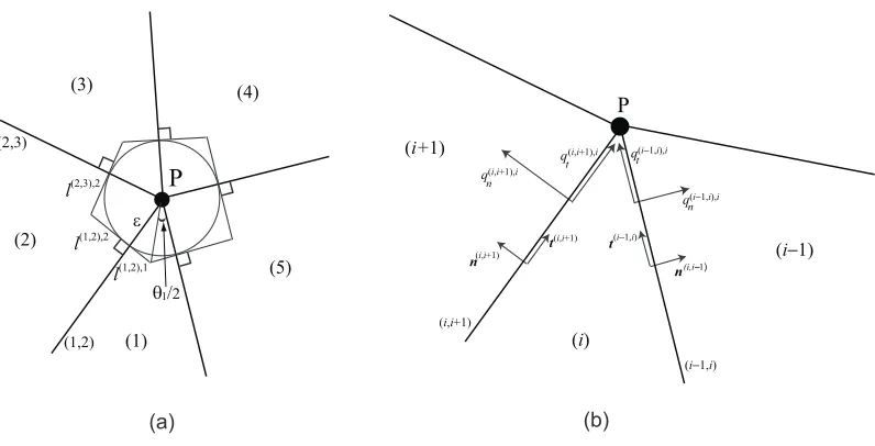
We denote byN the number of elements sharing an internal source node P in a triangular grid. There are
thereforeN interfaces intersecting at the node P. Figure 1(a) illustrates an internal node in a triangular
grid shared by N = 5 elements. The permeability tensors corresponding to each of the N elements
are denoted by Ki′j,i, i′, j = 1, d, where i = 1, N labels the element number. Let (i, i+ 1) denote the
interface between two neighbouring elements (i) and (i+ 1), and t(i,i+1) and n(i,i+1) the tangent and
the normal unit vectors to the interface (i, i+ 1), for i = 1, . . . , N (the elements are always counted
in a clockwise direction around the node). Using this notation, elements (N + 1) and (1) will be the
same, and so will be elements (0) and (N). The tangent unit vector t(i,i+1) is oriented toward the source
node P, and the normal unit vector n(i,i+1) is oriented outward from the element (i) over which the
integration is performed, toward the element (i+ 1), as represented in Figure 1(b), so that we have
t(i,i+1) = t(i+1,i) and n(i,i+1) = −n(i+1,i) (we denote by n(i+1,i) the normal unit vector to the (i, i+ 1)
interface for element (i+ 1)). The flux for an element (i) at node P can be uniquely written in terms of
these unit vectors as follows:
qi =qt(i,i+1),it(i,i+1)+q(i,i+1),i
n n
(i,i+1) (3)
or
qi =qt(i−1,i),it(i,i−1)+q(ni−1,i),in(
i,i−1) (4)
(for the (i−1, i) interface), where
qn(i,i+1),i =− ∂p
∂n+
!(i,i+1),i
=−
d
X
i′,j=1
Ki′j,icos(n, xi′)
∂p ∂xj
!(i,i+1),i
(5)
and
q(ti,i+1),i =−
∂p ∂t+
!(i,i+1),i
=−
d
X
i′,j=1
Ki′j,icos(t, xi′)
∂p ∂xj
!(i,i+1),i
(6)
denote the tangential and the normal component ofqi, respectively, with respect to the interface (i, i+1)
on element (i) at P, as indicated in Figure 1(b), with expression (4) following similarly for the interface
(i−1, i), and cos(n, xi′) and cos(t, xi′) are the direction cosines of the normal n and the tangent t to
the surface Γ, respectively.
Thus each flux componentqi is a linear combination of a tangential and a normal pressure gradient
com-ponent. Consequently, along each interface there are two tangential and two normal pressure gradient
components, arising from the two neighbouring elements.
However, there is an alternative representation ofqi in terms of only the tangential fluxes q(i,i+1),i
t and
qt(i−1,i),i which correspond to the elements (i−1) and (i+ 1) that neighbour the element (i), namely:
qi=γtt(i,i+1)+̺tt(i−1,i) (7)
where the expression for γt and ̺t can be found from the system of equations obtained by multiplying
equation (7) by t(i,i+1) and t(i−1,i) respectively and taking into account expressions (3) and (4):
γt+̺tt(i−1,i)·t(i,i+1) =qt(i,i+1),i
γtt(i,i+1) ·t(i−1,i)+̺t=q
(i−1,i),i t
The expressions for γt and ̺t are found to be
γt=
1
1−(t(i−1,i)·t(i,i+1))2q (i,i+1),i
t −
t(i−1,i)·t(i,i+1)
1−(t(i−1,i)·t(i,i+1))2q (i−1,i),i
t (9a)
̺t=
1
1−(t(i−1,i)·t(i,i+1))2q (i−1,i),i
t −
t(i−1,i)·t(i,i+1)
1−(t(i−1,i)·t(i,i+1))2q (i,i+1),i
t (9b)
Similarly, using the alternative representation of qi in terms of only the normal fluxes q(i,i+1),i
n and
q(i−1,i),i
n corresponding to the elements (i−1) and (i+ 1) that neighbour the element (i), we can write
qi =γnn(i,i+1)+̺nn(i−1,i) (10)
where γn and ̺n are found in a similar way toγt and ̺t, and their expression is given by
γn=
1
1−(n(i−1,i)·n(i,i+1))2q (i,i+1),i
n −
n(i−1,i)·n(i,i+1)
1−(n(i−1,i)·n(i,i+1))2q (i−1,i),i
n (11a)
̺n=
1
1−(n(i−1,i)·n(i,i+1))2q (i−1,i),i
n −
n(i−1,i)·n(i,i+1)
1−(n(i−1,i)·n(i,i+1))2q (i,i+1),i
n (11b)
The denominators in equations (9a), (9b), (11a) and (11b) are always non-zero, as the neighbouring
tangential or normal unit vectors cannot be parallel.
By using the different representations of qi given by equations (3), (4), (7) and (10), the following
equations can be obtained:
q(ti,i+1),it(i,i+1)+qn(i,i+1),in
(i,i+1) =γ
tt(i,i+1)+̺tt(i−1,i) (12a)
q(ti−1,i),it(i,i−1)+q(i−1,i),i
n n(i−1,i) =γnn(i,i+1)+̺nn(i−1,i) (12b)
and after all the flux components in these equations are replaced using equations (5) and (6), the two
normal pressure gradient components can be determined in terms of the tangential pressure gradient
components from these two conditions, in a similar way as they are determined in the case of a
rectan-gular internal source node (see Lorinczi et al. [2]). Thus at each node the number of unknowns at each
internal source node reduces to 2N + 1, namely 2N tangential pressure gradient components and the
pressure.
In a triangular grid, as in the case of a rectangular one, at each internal source node and for every
interface occurring at that node there is a condition representing the continuity of the tangential pressure
gradient at that interface. Together, these represent N different conditions, which reduce the number
of unknowns at each internal source node toN + 1.
In order to illustrate the conditions at each node, necessary to solve the system of unknowns, we consider
a small circle of radius ǫ, centred on the node, and the convex polygon which is formed by the tangents
to the circle at the points where the circle intersects the element interfaces, as shown in Figure 1(a).
Therefore each side of the polygon is perpendicular to the interface at that point. A generalised nodal
flux condition for each node in this case can be expressed by the relation:
N
X
i=1
(l(i,i+1),iqt(i,i+1),i+l(i,i+1),i+1q
(i,i+1),i+1
t )t(i,i+1) = 0 (13)
where l(i,i+1),i represents the length of the polygon side intersecting the interface (i, i+ 1) and situated
in element (i).
The nodal flux condition that we use is more restrictive than the mass conservation around a small
square enclosing a node. However, it has been shown in a range of problems in Lorinczi et al. [1] and
Lorinczi et al. [2] that it does not condition the type of solutions.
Equation (13) can be rewritten using the expressions of the tangential components of the flux and the
tangential pressure gradient continuity conditions as follows:
N
X
i=1 "
−l(i,i+1),i
d
X
i′,j=1
Ki′j,icos(t, xi′)
∂p ∂xj
!(i,i+1),i
−l(i,i+1),i+1
d
X
i′,j=1
Ki′j,i+1cos(t, xi′)
∂p ∂xj
!(i,i+1),i#
t(i,i+1) = 0
(14)
Because the polygon edges are tangent to the circle, every two edge segments situated in the same
element have the same length, namely
l(i,i+1),i=l(i−1,i),i, i= 1, . . . , N . (15)
We can determined these lengths as functions of the circle radiusǫand the angle between the neigbouring
interfaces. Ifθi denotes the angle between the interfaces (i−1, i) and (i, i+ 1), then we have
l(i,i+1),i =ǫtan θi 2
!
, i= 1, . . . , N (16)
Using equation (16) in equation (14) gives (as we take the limit asǫ →0)
N
X
i=1 "
−tan θi
2
! d X
i′,j=1
Ki′j,icos(t, xi′)
∂p ∂xj
!(i,i+1),i
−tan θi+1
2
! d X
i′,j=1
Ki′j,i+1cos(t, xi′)
∂p ∂xj
!(i,i+1),i#
t(i,i+1) = 0
(17)
Two conditions are included in relation (17), and they are obtained by resolving in thexandydirections.
We can further generateN−1 equations at each internal source node, by integrating in turn overN−1
node, a total of N+ 1 conditions can be generated, sufficient to determine the unknowns at that node.
After determining all of these unknowns, the set of tangential and normal components of flux at each
interface can be fully determined.
2.2
Side source node
We consider now boundary nodes and we refer to the side source node P in Figure 2(a). If N denotes
the number of elements sharing the source node P, then there areN−1 internal interfaces intersecting
at point P. Elements (1) and (N) are assumed to be the two elements on the boundary of the domain
for the node P. For each of these interfaces there will be one independent tangential component of the
pressure gradient, since a condition representing the continuity of the tangential pressure gradient at
that interface can be used. Consequently, there are N −1 unknown tangential components of the flux
at the internal boundaries. We can express the normal components of the pressure gradient for all the
internal interfaces in terms of the tangential components in the same manner as for the internal source
nodes in Section 4.1. For the two boundary interfaces, there is one tangential component of the flux for
each, corresponding to the single element to which each boundary interface belongs, and we denote by
qt1 andqN
t the fluxes for elements (1) and (N), respectively. The corresponding unit tangent vectors are
denoted byt(1) and t(N) =−t(1). The outward normal flux to the boundary, denoted by qn, is assumed
to apply at P for both elements (1) and (N) and is either specified (when the pressure is unknown at
P) or is an unknown (when the pressure is known at P). Thus, there are N + 3 unknowns at the side
source node P. The nodal flux condition (similar to condition (14)) incorporates the normal flux qnand
it is expressed in this case as follows:
l(1,2),1qt1t(1)+
N−1 X
i=1
l(i,i+1),iqt(i,i+1),i+l(i,i+1),i+1q
(i,i+1),i+1
t
t(i,i+1)+l(N−1,N),NqN t t(
N) = 2ǫq
nn (18)
which can be reformulated as
−tan θ1
2
! d X
i′,j=1
Ki′j,1cos(t, xi′)
∂p ∂xj
!(1)
t(1)+
N−1 X
i=1 "
−tan θi
2
! d X
i′,j=1
Ki′j,icos(t, xi′)
∂p ∂xj
!(i,i+1),i
−
tan θi+1 2
! d X
i′,j=1
Ki′j,i+1cos(t, xi′)
∂p ∂xj
!(i,i+1),i#
t(i,i+1)−tan θN
2
! d X
i′,j=1
Ki′j,Ncos(t, xi′)
∂p ∂xj
!(N)
t(N)= 2qnn
(19)
From equation (19) we can generate two conditions (in the x and y directions). Together with the
conditions obtained by integrating in turn over all of the elements sharing the side source node P and
the boundary condition at P, these represent the necessary N + 3 conditions for the unknowns at P to
be determined. The approach can be directly applied to corner points also.
3
Conclusions
In this article we have presented the generalisation of a numerical technique for solving steady-state
flow problems, namely the modified ‘q-based’ GEM for anisotropic media, to triangular elements. This
is an extension of the modified ‘q-based’ GEM has been developed for rectangular grids (Lorinczi et
al. [1]), the two techniques being based on the same concepts- satisfying a nodal flux condition at each
node and on the continuity of the tangential pressure gradient across the element boundaries.
The extension of the modified ‘q-based’ GEM for anisotropic media to triangular grids is still to be tested
in practice. However, this represents a useful theoretical advancement among the numerical solution
techniques for reservoir simulation.
Acknowledgement
Piroska Lorinczi would like to acknowledge the financial support received from the ORS and the Rock
Deformation Research Group, University of Leeds, UK.
References
[1] Lorinczi, P., Harris, S.D., Elliott, L. Modified flux-vector based GEM for problems in steady-state
anisotropic media. Eng Anal Bound Elem 2009; 33: 368−87, doi:10.1016/j.enganabound.2008.06.004.
[2] Lorinczi, P., Harris, S.D., Elliott, L. Influence of media properties on fluid flow in faulted and
fractured anisotropic media: a study using a modified flux-vector-based Green element method.
Transp Porous Med 2009; 80 : 469−498, DOI 10.1007/s11242-009-9376-3.
[3] Lorinczi P, Harris SD, Elliott L. Modelling of Highly-Heterogeneous Media Using a
Flux-Vector-Based Green Element Method. Eng Anal Boundary Elem 2006; 30: 818−33.
[4] Pecher R, Harris SD, Knipe RJ, Elliott L, Ingham DB. New formulation of the Green element
method to maintain its second-order accuracy in 2D/3D. Engineering Analysis with Boundary
Elements 2001; 25: 211−19.
Fig. 1. (a) An internal node in a triangular grid and (b) representation of the flux components and of unit
vectors for an element (i) in a triangular grid.
(1)
(3) (2)
P t
(1,2) n
(1,2)
q n
(a) (b)
P (1)
(2)
(3)
q n q
4 n
1
n (4) n
(1)
Fig. 2. (a) A side source node and (b) a corner source node in a triangular grid.
[image:9.595.102.500.133.336.2] [image:9.595.149.452.556.678.2]