Numerical simulation of cavitation and atomization using a fully compressible three-phase model

City, University of London Institutional Repository

Citation:

Mithun, M-G, Koukouvinis, P. ORCID: 0000-0002-3945-3707 and Gavaises, M.

ORCID: 0000-0003-0874-8534 (2018). Numerical simulation of cavitation and atomization

using a fully compressible three-phase model. Physical Review Fluids, 3(6), 064304. doi:

10.1103/PhysRevFluids.3.064304

This is the accepted version of the paper.

This version of the publication may differ from the final published

version.

Permanent repository link:

http://openaccess.city.ac.uk/20485/

Link to published version:

http://dx.doi.org/10.1103/PhysRevFluids.3.064304

Copyright and reuse: City Research Online aims to make research

outputs of City, University of London available to a wider audience.

Copyright and Moral Rights remain with the author(s) and/or copyright

holders. URLs from City Research Online may be freely distributed and

linked to.

City Research Online:

http://openaccess.city.ac.uk/

[email protected]

Numerical simulation of cavitation and atomization using a fully compressible

three-phase model

Mithun M G,∗ _{Phoevos Koukouvinis, and Manolis Gavaises}

School of Mathematics, Computer Science and Engineering, City, University of London, Northampton Square EC1V 0HB, UK

(Dated: May 23, 2018)

The aim of this paper is to present a fully compressible three-phase (liquid, vapour and air) model and its application to the simulation of in-nozzle cavitation effects on liquid atomization. The model employs a combination of homogeneous equilibrium barotropic cavitation model with an implicit sharp interface capturing VoF approximation. The numerical predictions are validated against the experimental results obtained for injection of water into the air from a step-nozzle, which is designed to produce asymmetric cavitation along its two sides. Simulations are performed for three injection pressures, corresponding to three different cavitation regimes, referred to as cavitation inception, developing cavitation and hydraulic-flip. Model validation is achieved by qualitative comparison of the cavitation, spray pattern and spray cone angles. The flow turbulence in this study is resolved using the Large Eddy Simulation approach. The simulation results indicate that the major parameters that influence the primary atomization are cavitation, liquid turbulence and, to a smaller extent, the Rayleigh-Taylor and Kelvin-Helmholtz aerodynamic instabilities developing on the liquid/air interface. Moreover, the simulations performed indicate that periodic entrainment of air into the nozzle occurs at intermediate cavitation numbers, corresponding to developing cavitation (as opposed to incipient and fully-developed cavitation regimes); this transient effect causes a periodic shedding of the cavitation and air clouds and contributes to improved primary atomization. Finally, the cone angle of the spray is found to increase with increased injection pressure but drops drastically when hydraulic-flip occurs, in agreement with the relevant experiments.

Keywords: Cavitation, atomization, LES, VoF, three-phase, compressible, step-nozzle, barotropic

I. INTRODUCTION

Fuel injectors are one of the major components of com-bustion engines as they control fuel delivery, atomization, mixing and to a large extent the combustion process. At-omization, in particular, is known to be influenced by the in-nozzle flow. Numerous studies have addressed ex-perimentally and numerically the formation and devel-opment of turbulence and cavitation inside fuel injectors and its effect on atomization [1, 2]. Despite considerable improvement in instrumentation technology, experimen-tation of the internal nozzle flow and spray breakup is challenging. Most of the relevant studies focus on scaled-up or simplified designs of real-size nozzles [3, 4]. Still, quantification of the liquid volume fraction and differ-entiation between the vapour and gaseous cavitation is an open question. On the contrary, numerical simula-tions, despite that high resolution required for capturing the very small turbulent and interfacial area scales, can provide insight regarding the flow dynamics at a resolu-tion that cannot be obtained with today’s experimental techniques.

Along these lines, one of the important factors to con-sider is the effect of turbulence on cavitation formation and development. Most of the relevant studies have utilised the Reynolds Averaged Navier-Stokes (RANS)

∗_{[email protected]}

equations for modelling turbulence owing to its simplic-ity and affordable CPU times. However, RANS models do not resolve the smaller vortices developing in the flow and thus, can significantly underestimate the formation and extent of cavitation [5]. Fixes such as the model of Reboudet al.[6] that compensate to a certain extent the increase of turbulent viscosity predicted by RANS turbu-lence models, do not have global validity. On the other hand, Large Eddy Simulations (LES) can be used to ob-tain a more accurate flow field, though at an increased computational cost. In LES, large-scale turbulence is re-solved, while scales below the grid size must be modelled. The comparative study of [5] involving different RANS and LES models suggests that RANS models fail to pre-dict incipient cavitation when the pressure difference be-tween inlet and outlet is low but LES can predict the formation of cavitation due to small vortices developing in the flow investigated.

Nomenclature u Velocity

c Speed of sound Sij Strain rate tensor

B Bulk modulus τ Non-dimensional time

Vn Nozzle mean velocity µ Kolmogorov length scale

p Pressure τµ Kolmogorov time scale

F Body forces ∇ Differential operator

t Time λg Taylor length scale

N Stiffness of Tait µt Turbulent viscosity

Cgas Constant of isentropic process for air τij Sub-grid scale stress

Cvap Constant of isentropic process for vapour ρsat,l Saturation density

W e Weber number psat,l Saturation pressure

lc Characteristic length δij Kronecker delta

Greek Symbols ν Kinematic viscosity

ρ Density Subscripts

σ Surface tension v Vapour

α Volume fraction g Gas

γ Heat capacity ratio for air l Liquid

κ Heat capacity ratio for vapour i, j, k Cartesian indices

the local velocity magnitude and only in very localised areas. The most widely utilised mixture approaches em-ploy a transport equation for the mass/volume fraction of the secondary phase. In this type of models, the phase-change rate is controlled using a source term which is typically derived from the Rayleigh-Plesset (R-P) equa-tion, as shown in [9–12]. A detailed review of such mod-els can be found in [13, 14]. The single-fluid approach for modelling cavitation uses an equation of state (EoS), which relates density and speed of sound with pressure and temperature. This simpler approach does not re-quire any transport equation for the secondary phase. A subset of this model is the barotropic model in which the density is assumed as a function of pressure alone. A barotropic model assumes pressure equilibrium and infi-nite mass transfer between the phases. Hence, it is also known as homogeneous equilibrium model. One limita-tion of such models is that they cannot predict the baro-clinic torque ((∇ρ× ∇p)/ρ2_{), since the density variation} is aligned with the pressure variation [15]. Another chal-lenge in modelling cavitation using barotropic models is defining an appropriate EoS for the mixture, which in-cludes air in addition to liquid and vapour. Despite these limitations, barotropic models are widely used for com-plex simulations due to their simplicity and numerical stability [5, 16].

The break-up of liquid jet occurs when the disruptive forces exceed the stabilising forces, such as surface ten-sion and viscous force. The disruptive forces arise from many internal and external factors such as liquid turbu-lence, cavitation in the nozzle and aerodynamic forces from the surrounding gas [17]. During injection, a race between the disruptive and stabilising forces produce in-stabilities which under certain condition get amplified leading to the disintegration of the liquid jet forming droplets. The break-up process that occurs near to the nozzle exit (prior to the formation of droplets) is fre-quently referred to as primary atomization. There have been many attempts to study numerically the

atomiza-tion process in the past; the numerical complexity is aris-ing from the multi-phase nature of the flow, the interac-tion between the phases and the sudden variainterac-tion in fluid properties across the interface. The numerical models developed in this front can be broadly classified into two main categories, one employing the Eulerian-Lagrangian (E-L) and the other using Eulerian-Eulerian (E-E) frame-work. In the E-L approach, the spray is represented as parcels containing a finite number of uniform droplets which are transported using Lagrangian formulation; the continuous gas phase is represented using Eulerian con-servation equations. The coupling between the phases is achieved through source terms for mass, momentum and energy exchange. One of the major limitations of the E-L model is its sensitivity to the mesh resolution espe-cially in the dense spray region [18]. Different method-ologies to circumvent the grid sensitivity can be found in [19–21]. On the other hand, the E-E models treat both phases as a continuum and solve conservation equations in the Eulerian framework. This approach provides bet-ter predictions in the dense spray region. Several studies employing the E-E framework can be found in [22–24] among many others. The Eulerian-Lagrangian spray at-omization (ELSA) [21, 25] and the Coupling Interface (ACCI) [26], implemented in AVL FIRE Code, take ad-vantage of both the E-L and E-E approaches by coupling them [27–29]. Another popular approach for modelling atomization is by employing a method that tracks the liquid-gas interface, such as the VoF, level-set or a cou-pled level-set/VoF [30, 31]. Such models are useful for modelling primary atomization where many topological changes such as interface pinching and merging occur and the interface motion are to be tracked accurately.

exten-sions of cavitation models accommodating for the addi-tional gas phase. Along these lines, the cavitation model of [32] was extended to an eight-equation, two-fluid model to include non-condensable gas by [33]. This model was then used to study the cavitating liquid jet problem in a two-dimensional step-nozzle. Another three-phase model based on the homogeneous mixture approach can be found in [34]. This model represents an extension of the single-fluid cavitation model of [16] to a closed-form barotropic two-fluid model and has been employed in LES simulations of a 3D step-nozzle. The authors reported three mechanisms responsible for the break-up of the liquid jet: turbulent fluctuations caused by the collapse of the cavity near the nozzle’s exit plane, air en-trainment into the nozzle and cavitation collapse events near the liquid-gas interface. An alternative approach for modelling the co-existence of three-phases is by employ-ing the Volume of Fluid (VoF), with a high-resolution interface capturing scheme such as the one of [35]; this approach can be advantageous for modelling atomiza-tion. To the author’s best knowledge, there are five stud-ies available in the literature that attempted to link a two-phase VoF model with a cavitation model for study-ing the in-nozzle effects on atomization [36–40]. These models differ in the way cavitation is resolved. A lin-ear barotropic model similar to the one presented in [41] was combined with VoF for modelling atomization in a gasoline injector by [38]. A comparative study between two transport-based cavitation models [10, 11] and em-ploying VoF can be found in [40] for a single-hole solid cone injector. Further studies that assume the phases to be incompressible can be found in [36, 39]. A Eulerian-Eulerian cavitation model with VoF was used to study cavitation and liquid jet break-up in a step-nozzle by [36]. The incompressible assumption in this study was justified by the low-pressure conditions used.

In this study, we present a three-phase model which considers compressibility of all the phases using non-linear isentropic relations. Such a consideration for com-pressibility is essential to capture the nonlinear effects of the flow even when phase-change is not dominant. In our model, the liquid compressibility is modelled using a modified Tait equation, which can predict the water den-sity and speed of sound with a minimum deviation (up to 0.001% for density and 3.8% for the speed of sound) from the experimental data [42]. As far as modelling the compressibility of the vapour phase is concerned, even though the vapour formation occurs below the satura-tion pressure, where compression can be considered to be negligible, the expansion of the vapour at this lower pressure plays an important role in the accuracy of the numerical model [43]. We utilised isentropic gas relation-ship for modelling the pure vapour and gas phase. The compressibility of the mixture phase is modelled using the Wallis speed of sound correlation. All three-phase models available in the literature and presented above, either consider the phases to be incompressible or assume linear compressibility, which results in much higher speed

of sound for the mixture phase (∼136 m/s compared to the 0.8 m/s using the present non-linear model at 50% vapour volume fraction with same fluid properties). Ac-cording to [44], during phase-change, the speed of sound should have a value between the frozen speed of sound 3m/s and equilibrium speed of sound 0.08m/s [45] which is achieved with the current model. To the best of au-thor’s knowledge, this is the first work to consider a non-linear compressible model in conjunction with VoF and LES for studying the in-nozzle effect on primary atom-ization. The current model also offers better numerical stability for the pressure based solver used by having the speed of sound and the density as a continuous function of pressure across the phases.

The paper presents a qualitative validation of the aforementioned three-phase model, including compar-isons of the in-nozzle cavitation and the spray forma-tion against experimental results from [46]. Three cav-itation regimes, namely cavcav-itation inception, developing cavitation and hydraulic-flip, have been considered. The simulations are focused on studying the interaction be-tween the in-nozzle cavitation and the primary atomiza-tion. The study has revealed that apart from cavitation, its secondary effects such as air entrainment into the noz-zle also have a greater influence on atomization and the consequent formation of the spray angle. It was also ob-served that the spray widening occurs twice during one entrainment cycle when developing cavitation occurs, one during the entrainment and other during push-out. The flow field of the periodic air entrainment into the nozzle is also presented in detail for the first time.

The structure of this paper is outlined as follows: The numerical method used for the three-phase equilibrium model is discussed in the next section, followed by the numerical simulation setup. Then the validation of the model along with major findings from the simulation are presented in the results and the discussion section; the main conclusions are summarised in the end.

II. MATHEMATICAL MODEL

A. Governing Equations

The three-phase flow is modelled using Volume of Flu-ids (VoF) approach which consider a cavitating fluid as the primary phase and the non-condensable gas (NCG) as the secondary phase. To track the interface between the two phases, a continuity equation for the secondary phase volume fraction as given in Eq. (1) is first solved. Then the volume fraction of the primary phase is calcu-lated using the constraint given in Eq. (2).

1 ρg

_∂(α gρg)

∂t +∇ ·(αgρgu¯g) =

X

( ˙mlv−g−m˙g−lv)

(1)

αlv+αg= 1 (2)

where,ρg,αgare the density and volume fraction of the

NCG. The termP_{( ˙m}

lv−g−m˙g−lv) is the mass transfer

between the two phases which is zero in the present study. The subscriptlv andg refers to the cavitating fluid and NCG respectively.

The mixture density (ρm) at each cell in the domain is

calculated as the weighted sum of individual phase den-sities as given in Eq. (3).

ρm= (1−αg)ρlv+αgρg (3)

In Eq. (3), the density of the cavitating fluid (ρlv) and

the NCG (ρg) is calculated using barotropic equations

of states and their calculations are described in the next section. Once the densities are calculated, the volume fraction of the pure vapour phase is computed using the relation:

αv =

(ρl−ρlv)

(ρl−ρv)

(4)

where, αv, is the volume fraction for the pure vapour

phase,ρlandρvare the density of liquid and pure vapour

at saturation.

Once all the mixture properties such as density and vis-cosity are calculated, a single set of momentum equation for the mixture phase is solved. The resulting velocity filed is then shared among all the phases. The filtered form of the momentum equation employed for the LES simulations is given in Eq. (5):

∂ρmu¯i

∂t +

∂ρmu¯iu¯j

∂xj

=−∂p¯ ∂xj

+ ∂

∂xj

µ(∂u¯i ∂xj

+∂u¯j ∂xi

)

+∂τij ∂xj

+F¯ (5)

In Eq (5), where,µis the molecular viscosity, ¯pis the filtered pressure, ¯F includes all body forces andτij is the

subgrid-scale stress defined as:

τij =−2µt(Sij−

1

3Sijδij) + 1

3τkkδkk (6)

In this study, the turbulent viscosityµtis modelled

us-ing Wall-Adaptus-ing Local Eddy-Viscosity model (WALE) [48] which has been proved in past studies [5] to be suit-able for wall-bounded flows. Sij in Eq. (6)] corresponds

to the strain rate tensor.

Since the flow is assumed to be isentropic and the com-pressibility of the fluid media is considered to be a func-tion of pressure alone, the solufunc-tion of energy equafunc-tion is not required.

B. Three-phase model

The three co-existing phases i.e. liquid, vapour and NCG (air) are modelled using a combination of a barotropic cavitation model coupled with the VoF ap-proach described above. The cavitation model used in

this study is a piecewise function employing three dif-ferent equations corresponding to liquid, liquid-vapour mixture and vapour phases. The Tait equation of state is used for modelling liquid (ρ ≥ ρl); the pure vapour

phase (ρ < ρv) is modelled using the isentropic gas

equa-tion and the equaequa-tion for the mixture phase (ρv ≤ρ≤ρl)

is derived by integrating Eq. (7) with respect to mixture density for an isentropic process, using the Wallis speed of sound [44] Eq. (8); the reader can refer to [5, 41] for the detailed derivation:

c2= (∂p

∂ρ)s (7)

1 c2

mρm

= αl c2

lρl

+ αv c2

vρv

(8)

where,c is the speed of sound andαis the volume frac-tion. The subscript m,v and l correspond to mixture, vapour and liquid phases respectively and the subscript srefers to an isentropic process.

p=      B

(_ρ ρ l(Tl))

N _{−1] +p}

sat,l ρ≥ρl

c2

vc2lρlρv(ρv−ρl)

c2

vρ2v−c2lρ2l

ln _c2 ρ

lρl(ρl−ρ)+c2vρv(ρ−ρv)+pref ρv≤ρ≤ρl

Cvapρκ ρ≤ρv

(9)

In Eq. (9), B is the bulk modulus,psat,l andN are the

saturation pressure and the stiffness of the liquid, respec-tively. The parameter pref in the mixture equation is

tuned to ensure continuous variation of density between the liquid and mixture phases. Cvap is the constant of

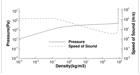
the isentropic process and is the heat capacity ratio for the vapour phase. Fig. 1 shows the behaviour of the equation of state Eq. (9) in a logarithmic plot between pressure and density. In this paper, the parameters for the Eq. (9) are set considering water as the working fluid.

FIG. 1. Two-phase barotropic relation (plot in log scale)

The third phase, i.e. the non-condensable gas is mod-elled as an additional phase, which is assumed to be im-miscible with the barotropic fluid. The pressure-density relationship for the non-condensable gas follows the isen-tropic gas equation of state as given in Eq. (10). Air at ambient condition (1bar and 293K) is considered as the gas here:

p=Cgasργ (10)

where, Cgas is the constant of the isentropic process for

air andγis the heat capacities ratio for air. The thermo-dynamic properties of water, vapour and gas (air) along with the constants used in Eq. (9) and Eq. (10) are listed in Table. I.

The barotropic fluid and the non-condensable gas equations (Eq. 9 and Eq. 10) are then combined using the implicit VoF model to closure the interaction of the three-phase system as described in the previous section. The discretisation of the phase volume fraction is per-formed using the compressive scheme of [47], which is a second-order reconstruction method, with slope limiter values ranging between 0 and 2. In the current study, a limiter value of 2 is used, which corresponds to the CICSAM (Compressive interface capturing for arbitrary meshes) scheme of [35].

An important interfacial factor that can impact the primary atomization is the surface tension between the

liquid and gas. In order to identify the influence of sur-face tension, a two-dimensional simulation on the same step-nozzle was performed with the same mesh resolution in Appendix. 2. The local Weber number at the primary atomization regions was considered as the judging pa-rameter. In the simulation, Weber numbers were in the range of 40, near the locations of primary atomization. Thus, the role of surface tension is prominent and thus, it has been considered in the 3D simulations. The con-tinuum surface force (CSF) approach of [49] was used for modelling surface tension and this has been included as an additional source term to the momentum equations of the VoF model. The model does not allow mixing be-tween the vapour and gas phases. However, this does not have much effect in the present study due to the fact that the vapour can exist only at low pressure (below satura-tion) and the air everywhere in the domain is always at a pressure higher than saturation pressure (air pressure is ambient or higher). When the air at a pressure higher than saturation pressure meets the vapour, the vapour will get compressed or condense back into liquid. This means that the vapour and gas cannot co-exist in the domain. The consideration of mixing becomes impor-tant where the non-condensable gas in the released form is modelled along with the liquid. For such studies, the present model can be extended by introducing a diffused interface model such as a mixture model which allows the mixing of phases, or a model with variable surface ten-sion between vapour and gas that diminishes when the density of the barotropic fluid falls below the saturation density of the liquid (water in this case) along with a reduced sharpness of the interface compression scheme.

III. SIMULATION CASES AND SETUP

Computations have been performed on the step-nozzle configuration of [46] for which experimental data for the in-nozzle flow and the near-nozzle atomization are avail-able. The geometry of the nozzle and the computational domain is shown in Fig. 2.

In order to visualize the evolution of the liquid jet, the flow field is initialized with zero velocity throughout the domain while constant pressures are applied at the inlet and outlet boundaries. The extended cylindrical region at the exit is initialized with 100% gas volume fraction (αg= 1) to model the presence of ambient air.

TABLE I. Thermodynamic properties for water, vapour and gas at 20o_C.

Liquid properties Vapour properties Gas properties

B 3.07 GPa Cvap 27234.7 P a/(Kg/m3)n Cgas 75267.8 Pa/(Kg/m3)

N 1.75 – κ 1.327 – γ 1.4 –

ρsat,L 998.16 Kg/m3 ρsat,V 0.0173 Kg/m3

Csat,L 1483.26 m/s Csat,V 97.9 m/s

Psat,L 4664.4 Pa Psat,V 125 Pa

µL 1.02e-03 Pas µV 9.75e-06 Pas µg 1.78e-5 Pa s

Surface tension 0.0728 N/m

FIG. 2. a) Step- Nozzle geometry as reported in Abderrez-zak and Huang [46] b) Computational domain with boundary conditions; walls (grey), inlet (red), and outlet (blue). All dimensions are in millimetres.

of the nozzle passage is included. The nozzle has a non-uniform inlet with a step of 1mm on one side, to trigger an asymmetry to cavity formation. The absolute value of the inlet and outlet pressure are set corresponding to the experimental conditions presented in [46]. The abso-lute pressure at the outlet is fixed at 1 bar and the inlet total pressure is adjusted to match different static pres-sures between inlet and outlet. The boundary conditions used for the current simulations are listed in Table. II. It should be noted that since the flow rate measurements

TABLE II. Boundary conditions used for the simulation Inlet pressure

(pin)absin bar

Mean Velocity of water in the noz-zleVnin m/s

Reynolds number

2.0 13.5 64586

3.0 18.3 89540

5.0 25.9 126727

were not reported in the reference paper and the pres-sure meapres-surements are reported further upstream, a cor-rection of 0.5bar is applied at the computational inlet to compensate for the pressure drop in the inlet tubing system. The inlet pressure is calibrated such that the cavitation regimes are matched between the experiments and computations.

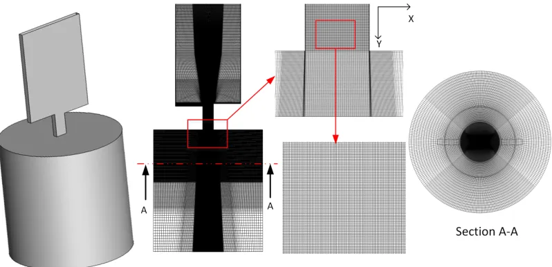
The computational mesh used for the simulation is shown in Fig. 3. A block-structured mesh with appropri-ate refinement near the walls is used to ensureY+ <1. The initial estimate of the mesh resolution for LES sim-ulation is calculated based on the Kolmogorov (Eq. (11)) and Taylor (Eq. (13)) scales (refer to [2, 5, 50, 51]:

µ= (ν3/)14 ∼_{0.84µm (11)}

τµ= (ν/) 1

2 ∼0.7µs (12)

γg =

√

10Re−0.5L∼48µm (13)

In the above equations, ν is the kinematic viscosity of water (∼ 10−6m2/s), is the turbulent dissipation calculated as u3/L, with u being the average velocity through the nozzle andLthe characteristic length (width of nozzle = 5 mm). In order for the mesh resolution to be sufficient for all the inlet pressures values considered, the flow parameters (such as average velocity) at the extreme condition is used. In this study, an average velocity of 22.2 m/s corresponding to a pressure difference of 5bar across inlet and outlet as reported in [46] is considered.

FIG. 3. Details of the computational mesh.

of the nozzle, the total mesh count in the domain sums to∼15million cells. The time resolution is controlled by using an adaptive time stepping method so as to main-tain the Courant - Friedrichs - Lewy (CFL) number to be less than 0.8 throughout the computational domain.

In the results that follow, the variables are made non-dimensional based on the mean velocity inside the nozzle corresponding to each condition (reported in Table. II) and the width of the nozzle (Wn). Using this approach the non-dimensional time takes the form (τ =tVn/Wn).

IV. RESULTS AND DISCUSSION

A. Comparison of in-nozzle cavitation and spray with experiments

A comparison of the in-nozzle flow and the near-exit spray formation between the experimental results from [46] and the present computations are shown in Fig. 4. The results are presented for three different injection pressure conditions, each corresponding to three differ-ent cavitation regimes. The first condition considered in this study corresponds to the case where cavitation incep-tion occurs (at 2bar injecincep-tion pressure). The incepincep-tion of vapour cavity is observed from the lower wall with very little or no cavitation from the upper wall. The results presented in Fig. 4 confirm that the liquid jet atomises faster on the cavitating side of the step-nozzle as more ligaments and droplets forming on this side. Looking to the second condition at 3bar, the cavity formed at the inlet corner of the lower wall extends up to 70% of the nozzle length while cavity formation is also seen from the upper wall (see Fig. 4c and d). Under this condition, pe-riodic shedding of vapour clouds is observed from both corners. With the increase in the intensity of cavitation,

a wider jet with finer droplets is formed. Compared to the experiments, the numerical simulation also shows the entrainment of ambient air moving backwards inside the orifice. As the injection pressure is further increased to 5bar, hydraulic-flip is observed, as liquid is completely separated from the lower wall allowing for ambient gas to flow inside the nozzle, as depicted in Fig. 4(e and f). The qualitative comparison shows a good match between the experimental results and simulations for all conditions.

B. Half-cone angle

FIG. 4. Comparison of in-nozzle cavitation and near-exit spray formation between experimental results from Abderrezzak and Huang [46] and current numerical study. (a, b) 2bar (c, d) 3bar (e, f) 5bar inlet pressure. Iso-surfaces of mixture density at 100kg/m3 shown at a random time instant

geometric features, for example, a curvature at the exit plane of the experimental geometry can lead to a wider spray as compared to the sharp edges considered in the CFD model.

C. Evolution of in-nozzle flow and liquid jet

In this section, results are presented to show the in-nozzle flow effects on liquid jet evolution and atomiza-tion. The three conditions representing three cavitation regimes, namely, cavitation inception, developing cavi-tation and hydraulic-flip are given in Fig. (6 - 8). Re-sults are further supported from the presentation of the iso-surfaces of the turbulent structure represented by the second invariant of velocity gradient tensor (Q-criterion) [52, 53] given in Fig. (9 - 11) for the three flow condi-tions, respectively. Positive values of the Q-criterion can be used for identifying vortices and the local rotational areas. The iso-surface of the Q-criterion with a value of 109s−2 coloured with velocity magnitude is plotted to identify the evolution of vortical structures inside the nozzle.

Cavitation inception is the condition at which the cavi-tation first occurs; the 2bar case can be considered rep-resentative of this change in the flow (see, Fig. 6). As the flow progresses, the formation of a small vapour cavity can be observed from the sharp corner of the lower wall. This is then convected by the flow towards the nozzle exit and mostly collapses within the nozzle. Only neg-ligible amount of vapour formation is observed from the upper wall at this pressure condition. Turning now to the emerging jet evolution, during the early stages of injec-tion, the formation of a mushroom-shaped liquid can be observed at the leading-edge due to the Rayleigh-Taylor instability caused by the density difference [54, 55]. Fur-ther, the interaction between the large inertia liquid mov-ing outwards and the ambient gas, shearmov-ing the liquid due to the pressure gradient at the jet front also assist in the mushroom formation [56]. As the flow progresses, the mushroom grows in size and a larger recirculation zone of gas is created behind it. This recirculation initiates the necking of the jet behind the mushroom, which leads to the formation of droplets (Fig. 6 b-c). The forma-tion of liquid droplets is first observed from the edge of the mushroom and later from the core of the liquid jet. The small circumferential waves seen around the liquid jet are initiated by the aerodynamic Kelvin-Helmholtz (K-H) instability developing at the liquid-air interface. It has been reported that the influence of aerodynamic forces on the primary breakup of the liquid jet is negli-gible if the density ratio (ratio of liquid over air density) is greater than 500. In such flow, the breakup is pri-marily due to the liquid turbulence [57]. In the present study, the density ratio is 1000; with almost no cavita-tion occurring at this pressure condicavita-tion, the breakup of the liquid jet can be primarily attributed to liquid tur-bulence. The turbulent structures inside and outside the

nozzle are depicted in Fig. 9 by plotting the Q-criterion. The interaction of the turbulent structures with the liq-uid jet surface initiating the disruption of the liqliq-uid core can be seen while comparing two time instances, one at an early stage when turbulent structures are still inside the nozzle where the liquid surface only shows K-H waves (Fig. 6c and Fig. 9b) and another instance when the tur-bulent structures leave the nozzle and interact with the liquid-air interface, where the interface becomes irregu-lar leading to the formation of ligaments (Fig. 6d and Fig. 9c). The collapse of the vapour clouds that are con-vected beyond the nozzle exit further assists in the disin-tegration of the liquid; formation of liquid ligaments can be observed in Fig. 6e onwards. Due to the asymmetry in the geometry creating more cavity formation from the lower wall, the formed spray is spreading more in the di-rection of the lower wall. Widening of spray cone angle with increasing cavitation has been observed in other ex-perimental studies; see for example [46],[1],[58].

A developing cavitation with the periodic shedding of vapour cavities is seen when the injection pressure is in-creased to 3bar; the process is depicted in Fig. 7. As expected, the cavitation from both walls increases with increase in injection pressure. The sheet cavity formed from the sharp inlet edge of the bottom wall quickly transforms into small vortices, which are then trans-ported by the flow. The variation in vortex transport velocity causes these vortices to merge together to form cavity clouds, at approximately 1/3rd _{downstream from}

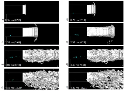
FIG. 6. Instances of the evolution of in-nozzle cavitation and liquid jet disintegration atpinj=2bar. Iso-surfaces of 50% vapour

(cyan) and 95% gas (white) volume fraction shown. The instances are chosen randomly over the evolution to highlight the main features. (The non-dimensional time is given in brackets)

widening of the liquid jet can be observed again in Fig. 7g (highlighted with blue circle). A similar observation was also made by [36], where the dynamic change in spray cone angle is reported over time. In short, during devel-oping cavitation, a periodic phenomenon of air entering and leaving the nozzle have been observed along with two events of spray widening and one event causing a reduction in spray width. The early evolution of the jet under this condition is like the previous 2bar case. The formation of a mushroom-shaped jet front and the initial droplet formation from its circumference can be also ob-served under this condition. However, the mechanism of the jet atomization, in this case, is primarily due to cavi-tation and air entrainment. Due to the increased velocity of the jet, the disintegration of liquid jet occurs earlier and closer to the nozzle exit.

At 5bar injection pressure, complete separation of the liquid flowing over the sharp edge corner of the lower wall is observed (Fig. 8). This condition is typically known as ”hydraulic-flip”. The higher injection pressure forces the flow to accelerate more around the nozzle inlet resulting in more vapour generated from both walls. Unlike the other two conditions presented, the formation of a sheet cavity can be seen from both walls at this pressure con-dition. The sheet cavity formed from the upper walls grows roughly up to 40% of the channel length until the

FIG. 7. Instances of the evolution of in-nozzle cavitation and liquid jet disintegration atpinj=3bar. Iso-surfaces of 50% vapour

(cyan) and 95% gas (white) volume fraction shown. The instances are chosen randomly over the evolution to highlight the main features. The thinning and widening of the liquid jet are highlighted using red and blue circles. (The non-dimensional time is given in brackets)

D. In-nozzle turbulence

The influence of turbulence on the atomization is demonstrated using the Q-criterion with a value of 109s−2, coloured with the non-dimensional velocity mag-nitude for the three injection pressures considered. The initial formation of spanwise vortices, stretching of vor-tices in the longitudinal direction and its subsequent transformation into hair-pin vortices can be seen in Fig. (9 - 11). To highlight the influence of turbulence on jet disintegration, a picture of the jet interface corre-sponding to that time is given as a subset of (b, c). The Fig. 9-11(a, b) corresponds to an early time instant where the in-nozzle turbulent structures are within the nozzle. At this condition, the jet interface only shows evidence of K-H waves. When the turbulent structures leave the nozzle, it interacts with the interface producing more dis-turbances on the interface initiating disintegration of the jet as can be seen from Fig. (9 -11)c. The presence of the entrained air in the nozzle close to the bottom wall produces more turbulence in this region, Fig. 10d and Fig. 11d.

E. Effect of air entrainment on jet

This section describes the process of air entrainment, primarily focusing on the events leading to widening and narrowing of the spray atpinj=3bar. During one air

FIG. 8. Instances of the evolution of in-nozzle cavitation and liquid jet disintegration atpinj=5bar. Iso-surfaces of 50% vapour

(cyan) and 95% gas (white) volume fraction shown. (The non-dimensional time is given in brackets)

FIG. 9. Instantaneous isosurface of Q-criteria showing vortex cores (value of 109) coloured by non-dimensional velocity mag-nitude atpinj=2bar. (The jet interface close to the nozzle exit is shown in subset).

flow area creating an additional component of velocity in the downward direction thereby increasing the spray angle, shown in Fig. 12d. The process of air entrainment and push-out occurs over a time-period of approximately 1.1ms (computed based on two cycles) and the process is

FIG. 10. Instantaneous isosurface of Q-criteria showing vortex cores (value of 109) coloured by non-dimensional velocity magnitude atpinj=3bar. (The jet interface close to the nozzle exit is shown in subset).

FIG. 11. Instantaneous isosurface of Q-criteria showing vortex cores (value of 109) coloured by non-dimensional velocity magnitude atpinj=5bar. (The jet interface close to the nozzle exit is shown in subset).

F. Time-averaged fields

Fig. 13 shows the average and rms field for the vapour volume fraction obtained from the statistics collected over 3ms. The vapour volume fraction clearly shows an increase in average cavitation development with a rise in injection pressure. There is only a negligible amount of vapour cavity formation at 2bar injection pressure (with a max volume fraction of 0.02 near the inlet edge). From 3bar to 5bar, an increase in the intensity and the spread of cavitation is visible, due to the increased acceleration of the flow near the inlet corner. The predicted rms val-ues of the vapour volume fraction are larger than the mean values, which implies a highly fluctuating cavity.

Similar observations can also be made for the gas en-trainment into the nozzle, with no enen-trainment at all at pinj=2bar to almost 70% towards the inlet at 3bar and

FIG. 12. Contours of non-dimensional velocity magnitude with iso-lines of 95-99% gas volume fraction. a) Pictorial represen-tation of the first spray widening event. (b, d) shows the widening of spray and c) shows the reduction in spray width. (the vectors shown are not up to scale they are used as an indicator of flow directions.

FIG. 14. Contours of mean and rms absolute pressure normalised with the injection pressure and iso-lines of gas volume fraction ranging from 0.1 - 0.5 at (a, d) 2bar, (b, e) 3bar and, (c, f) 5bar injection pressure.

the separated boundary layer from this wall to reattach quickly, before it reaches the mid-channel. Whereas, the flow separated from the bottom wall reattach at about 1/10thbefore the nozzle exit for 2bar and almost at the exit for 3bar. At 5bar, the separated shear layer from the bottom wall never reattaches. The velocity profile observed for 5bar injection pressure shows a different be-haviour compared to the other cases. The averaged field show a wavy vertical profile up to 20% of the nozzle width at the mid-plane (Y2) and the mean velocity at the exit plane (Y4), close to the bottom wall is lesser than the other cases, Fig. 15(h, i). This is due to the upstream motion of the entrained air during hydraulic-flip. Sim-ilarly, the entrainment of the gas also produces highly fluctuating velocity field near the bottom wall which is evident from the rms velocity profile shown in Fig. 15(j-l) with maximum fluctuations occurring at 3bar injection pressure near the nozzle exit.

The instantaneous field of the flow velocity and the vorticity at the mid-span (z-plane) of the nozzle for 5bar injection pressure are shown in Fig. 16, highlighting the mid and the near exit region of the nozzle. A closer look at the figure reveals that in addition to the water getting separated from the inlet, the air entering the noz-zle through the exit also separates from the exit corner

and reattach to the wall before reaching the mid-section of the nozzle. This creates a recirculation zone of air near the nozzle exit leading to the velocity distribution shown in Fig. 15i. The shear force between the liquid jet, the entrained gas and small droplets created in the near-wall separated region enhances turbulent produc-tion and a large number of smaller eddies are generated as can be seen from Fig. 16b and the mean vorticity con-tours shown in Fig. 15f. The wavy velocity profile inside the separated shear layer in Fig. 15h is the result of the continuous presence of these counter-rotating eddies.

G. Surface area generation

The quantification of the primary atomization is achieved by integrating the surface area of 50% gas vol-ume fraction over a volvol-ume of interest as a function of time. The results obtained from the integration is plot-ted against the non-dimensional time (τ =tVn/lref) for

FIG. 16. Instantaneous contours of (a,c) flow velocity in y-direction showing the flow separation of liquid from inlet edge and ambient gas from the exit edge of the bottom wall, (b) the instantaneous vorticity contours at 5bar injection pressure.

is refined enough to capture the primary atomization. At the start of injection, only the leading edge of the jet is exposed to ambient air and the surface area cal-culated is close to zero. The increase in surface area is observed at two different rates (two different slopes of the curve). The initial slope of the curves corresponds to the increase in surface area generation due to the forma-tion and expansion of the mushroom and the exposure of the liquid core to the ambient air due to liquid penetra-tion with time. Further increase in the slope is observed at the start of the liquid core disintegration (observed at τ ∼ 2.48 for 5bar, τ ∼ 7.74 for 3bar and τ ∼ 6.89 for 2bar). The surface area increases until the jet front reaches the end of the blue region (up to which integra-tion is performed), after which the curve drops due to the front mushroom leaving out of the integration do-main (line L1). For 5bar injection pressure, the start of air entrainment occurs at the non-dimensional timeτ ∼ 2.48 where the liquid bulk disintegration starts (where the slope increases) and the flow go into complete flip at τ∼4.25. At this time instant, the jet front is still within the integrating region and the surface area continue to increase due to the combined effect of primary atomiza-tion, the expansion of the mushroom front and the jet penetration (up to L1 whereτ ∼6.21). As the jet front leaves the domain (τ ∼6.21), there is a sudden drop in

the least favourable condition for primary atomization.

V. CONCLUSIONS

A numerical framework for modelling the co-existence of three-phases namely liquid, vapour and non-condensable gas has been developed. The model was utilised to study the effect of in-nozzle flow parameters, such as cavitation, on primary atomization of a liquid jet. A homogeneous equilibrium based barotropic approach is used for modelling cavitation, combined with a sharp in-terface Volume of fluid (VoF) method to complete the three-phase system. A wall adaptive LES was used for resolving turbulence.

The results from the simulations have been compared with the experimental results from [46] for three different cavitation regimes, namely cavitation inception, develop-ing cavitation and hydraulic flip. From the analysis, it has been observed that the disintegration of the liquid jet is influenced mainly by four factors: in-nozzle cavitation, the entrainment of air into the nozzle, the turbulence generated and partially due to the aerodynamic insta-bilities. The formation of the droplets is first observed from the mushroom edge due to Rayleigh-Taylor instabil-ities and later from the liquid core due to the combined effect of cavitation, turbulence and KelvHelmholtz in-stabilities. Liquid ligaments are formed when the vapour cloud collapses near the liquid-air interface. At cavita-tion incepcavita-tion, the atomizacavita-tion is primarily due to liquid turbulence and aerodynamic instabilities. Whereas at de-veloping cavitation, in addition to the above parameters, the cavitation and the air entrainment into the nozzle plays the major role. The air entrainment into the noz-zle is periodic when developing cavitation occurs. During one entrainment cycle, the spray cone angle is increased twice improving the atomization. Due to the asymmetry in the nozzle geometry, a partial hydraulic flip occurs at 5bar injection pressure, suppressing the vapour forma-tion from the lower wall completely. At this condiforma-tion, the atomization and the subsequent spray cone angle is drastically reduced.

From the observed results for three cavitation regimes considered, it can be concluded that the developing cavitation is the most favourable condition for effective atomization and wider spray. However, merging of vortices forming highly erosive potential vapour clouds has also been observed at this condition. Hence, there should be a trade-off between the cavitation-assisted atomization and erosion while designing an efficient nozzle. This study provides new insights in the less explored area of atomization by providing a framework for simultaneous simulation of the in-nozzle flow and primary atomization by utilising a barotropic model for cavitation, a surface tracking model for atomization and LES model for turbulence resolution.

ACKNOWLEDGMENTS

The research leading to these results has received fund-ing from the MSCA-ITN-ETN of the European Union’s H2020 programme, under REA grant agreement no. 642536. The authors would also like to acknowledge the contribution of The Lloyd’s Register Foundation. Lloyd’s Register Foundation helps to protect life and property by supporting engineering-related education, public engage-ment and the application of research.

Appendix

1. Grid resolution for LES

FIG. 17. Non-dimensional surface area generation (an approximate measure of primary atomization) at different injection pressures. The region where integration is performed is highlighted in blue (in the inset).

FIG. 18. LES resolution assessment (a) contour of the resolved over total turbulent kinetic energy at mid-span section and (b) along vertical location at giver locations, (c) Wall Y-plus. All plots are for the extreme condition considered in this study (Pinj=5bar).

2. Comparison between the mixture and VoF approach for three-phase modelling and the

influence of surface tension.

Here we present a two-dimensional study conducted on the same nozzle as presented in the paper with the same grid resolution with an objective to compare two differ-ent approaches for modelling the additional gas phase,

objec-]

FIG. 19. Turbulent energy spectra at mid- section of nozzle (left column) and 5mm downstream the nozzle-exit in spray region (right column) for (a, b) 2bar, (c, d) 3bar and (e, f) 5bar injection pressure.

FIG. 21. Instantaneous contours of (a) vorticity and (b) velocity magnitude from two-dimensional simulation using the mixture model (without surface tension effects). (c) The calculated Weber numbers at the highlighted regions.

tives, a laminar flow approximation is made in order to simplify the problem. A comparison between the pre-dictions from the two approaches (the mixture approach and the VoF approach) is given in Fig. 20 with an injec-tion pressure of 3bar applied at the inlet. It should be noted that the mixture model used in this study does not take into account the surface tension between the water and air. This is not a limitation of the mixture model, but a choice we made for comparing the effect of sur-face tension with a VoF model where a sursur-face tension of 0.0728N/m is assumed at the water-air interface. Some studies utilising the surface tension for a diffused inter-face mixture model can be found in [67], [68] and [69]. It is observed that the larger structures are well captured using both approaches. However, the smaller structures such as water ligaments and droplet formations are not captured well using the mixture model. The effect of sur-face tension is apparent in the smaller structures, where

the Kelvin-Helmholtz instabilities produce shallow struc-tures at the interface when surface tension is not present, as highlighted in Fig. 20a, whereas more flatten edges with thin ligaments can be observed in Fig. 20b when surface tension is present. This was further examined by estimating the local Weber number in the primary at-omization region. In Fig. 21, the contours of the instan-taneous vorticity and the velocity magnitude are shown, highlighting the regions where the Weber number is cal-culated, and the calculated values are given as a table in ig. 21c. The low Webber number values calculated (W e ∼ 20 to 40) indicates that the surface tension can have a significant effect on the spray structure, hence it is considered for the three-dimensional simulations psented. The Weber number is calculated using the re-lation W e= (ρgv2lc)/(σ), where lc is the characteristic

length, v is the local velocity magnitude and σ is the surface tension.

[1] M Gavaises, D Papoulias, A Andriotis, E Giannadakis, and A Theodorakakos, “Link Between Cavitation Devel-opment and Erosion Damage in Diesel Injector Nozzles,” inSAE Paper 2007-01-0246, Vol. 2007 (2007) pp. 776– 790.

[2] F Payri, V Berm´udez, R Payri, and FJ Salvador, “The influence of cavitation on the internal flow and the spray characteristics in diesel injection nozzles,” Fuel83, 419– 431 (2004).

[3] T Hayashi, M Suzuki, and M Ikemoto, “Visualization of Internal Flow and Spray Formation with Real Size Diesel Nozzle,” in ICLASS(Heidelberg, Germany, 2012). [4] N Mitroglou, M Gavaises, JM Nouri, and C Arcoumanis,

“Cavitation Inside Enlarged and Real-Size Fully Trans-parent Injector Nozzles and Its Effect on Near Nozzle

Spray Formation,” (2004) pp. 552–567.

[5] P Koukouvinis, H Naseri, and M Gavaises, “Performance of turbulence and cavitation models in prediction of in-cipient and developed cavitation,” International Journal of Engine Research , 146808741665860 (2016).

[6] JL Reboud, B Stutz, and O Coutier-Delgosha, “Two phase flow structure of cavitation: experiment and mod-eling of unsteady effects,” 3rd International Symposium on Cavitation CAV199826(1998).

[7] E Lauer, XY Hu, S Hickel, and NA Adams, “Numeri-cal investigation of collapsing cavity arrays,” Physics of Fluids24, 52104 (2012).

En-gineering125, 963–969 (2004).

[9] A Kubota, H Kato, and H Yamaguchi, “Finite difference analysis of unsteady cavitation on a two-dimensional hy-drofoil,” inFifth International Conference on Numerical Ship Hydrodynamics (1990).

[10] RF Kunz, DA Boger, DR Stinebring, S Chyczewski, JW Lindau, HJ Gibeling, S Venkateswaran, and TR Govin-dan, “A preconditioned Navier - Stokes method for two-phase flows with application to cavitation prediction,” Computers & Fluids29, 849–875 (2000).

[11] GH Schnerr and J Sauer, “Physical and Numerical Mod-eling of Unsteady Cavitation Dynamics,” in Fourth In-ternational Conference on Multiphase Flow (2001) pp. 1–12.

[12] PJ Zwart, AG Gerber, and T Belamri, “A Two-Phase Flow Model for Predicting Cavitation Dynamics,” in ICMF 2004 International Conference on Multiphase Flow (Yokohama, Japan, 2004).

[13] A Niedzwiedzka, GH Schnerr, and W Sobieski, “Review of numerical models of cavitating flows with the use of the homogeneous approach,” Archives of Thermodynamics

37, 71–88 (2016).

[14] T Goel, J Zhao, S Thakur, R Haftka, and W Shyy, “Sur-rogate Model-Based Strategy for Cryogenic Cavitation Model Validation and Sensitivity Evaluation,” in 42nd AIAA/ASME/SAE/ASEE Joint Propulsion Conference & Exhibit, Joint Propulsion Conferences (American In-stitute of Aeronautics and Astronautics, 2006).

[15] S Gopalan and J Katz, “Flow structure and model-ing issues in the closure region of attached cavitation,” Physics of Fluids Joint Propulsion Conferences,12, 895– 911 (2000), arXiv:arXiv:1011.1669v3.

[16] CP Egerer, S Hickel, SJ Schmidt, and NA Adams, “Large-eddy simulation of turbulent cavitating flow in a micro channel,” Physics of Fluids26, 085102 (2014). [17] H Lefebvre and GM Vincent, Atomization and Sprays,

Second Edition (CRC Press, 2017).

[18] XX Jiang, GA Siamas, K Jagus, and TG Karayiannis, “Physical modelling and advanced simulations of gas-liquid two-phase jet flows in atomization and spray,” Progress in Energy and Combustion Science36, 131–167 (2010), arXiv:fld.1 [DOI: 10.1002].

[19] P B´eard, J-M Duclos, C Habchi, G Bruneaux, K Mokad-dem, and T Baritaud, “Extension of Lagrangian-Eulerian Spray Modeling: Application to High Pressure Evaporating Diesel Sprays,” (2000).

[20] AM Lippert, S Chang, S Are, and DP Schmidt, “Mesh Independence and Adaptive Mesh Refinement For Ad-vanced Engine Spray Simulations,” (2005).

[21] W Ning, RD Reitz, AM Lippert, and R Diwakar, “De-velopment of a Next-generation Spray and Atomization Model Using an Eulerian- Lagrangian Methodology,” International Multidimensional Engine Modeling User’s Group Meeting (2007).

[22] A Behzadi, R I Issa, and H Rusche, “Modelling of dis-persed bubble and droplet flow at high phase fractions,” Chemical Engineering Science59, 759–770 (2004). [23] VA Iyer, J Abraham, and V Magi, “Exploring injected

droplet size effects on steady liquid penetration in a Diesel spray with a two-fluid model,” International Jour-nal of Heat and Mass Transfer45, 519–531 (2002). [24] M Vujanovi´c, Z Petranovi´c, W Edelbauer, J Baleta, and

Neven Dui´c, “Numerical modelling of diesel spray using the Eulerian multiphase approach,” Energy Conversion

and Management104, 160–169 (2015).

[25] A Vallet, AA Burluka, and R Borghi, “Development of a eulerian model for the atomization of a liquid jet,” Atomization and Sprays11(2001).

[26] AVL,Fire Manual, Tech. Rep. (2013).

[27] M De Luca, A Vallet, and R Borghi, “Pesticide atomiza-tion modeling for hollow-cone nozzle,” Atomizaatomiza-tion and Sprays19, 741–753 (2009).

[28] M Vujanovi´c, Z Petranovi´c, W Edelbauer, and N Dui´c, “Modelling spray and combustion processes in diesel en-gine by using the coupled EulerianEulerian and Euleri-anLagrangian method,” Energy Conversion and Manage-ment125, 15–25 (2016).

[29] Y Wang, WG Lee, RD Reitz, and R Diwakar, “Nu-merical Simulation of Diesel Sprays Using an Eulerian-Lagrangian Spray and Atomization (ELSA) Model Cou-pled with Nozzle Flow,” (2011).

[30] A Berlemont, Z Bouali, J Cousin, P Desjonqueres, M Doring, and E Noel, “Simulation of liquid/gas in-terface break-up with a coupled Level Set/VOF/Ghost Fluid method,” inICCFD7 (Big Island, Hawaii, 2012) p. 12.

[31] M Arienti, X Li, MC Soteriou, CA Eckett, M Suss-man, and RJ Jensen, “Coupled Level-Set/Volume-of-Fluid Method for Simulation of Injector Atomization,” Journal of Propulsion and Power29, 147–157 (2012). [32] R Saurel, F Petitpas, and R Abgrall, “Modelling phase

transition in metastable liquids: application to cavitating and flashing flows,” Journal of Fluid Mechanics607, 313– 350 (2008).

[33] Y Wang, L Qiu, RD Reitz, and R Diwakar, “Simulat-ing cavitat“Simulat-ing liquid jets us“Simulat-ing a compressible and equi-librium two-phase flow solver,” International Journal of Multiphase Flow63, 52–67 (2014).

[34] F ¨Orley, T Trummler, S Hickel, MS Mihatsch, SJ Schmidt, and NA Adams, “Large-eddy simulation of cav-itating nozzle flow and primary jet break-up,” Physics of Fluids27(2015), 10.1063/1.4928701.

[35] O Ubbink, Numerical Prediction of Two Fluid Systems With Sharp Interfaces, Phd thesis, Imperial College of Science, Technology and Medicine (1997).

[36] W Edelbauer, “Numerical simulation of cavitating injec-tor flow and liquid spray break-up by combination of Eulerian-Eulerian and Volume-of-Fluid methods,” Com-puters and Fluids144, 19–33 (2017).

[37] M Ghiji, L Goldsworthy, PA Brandner, V Garaniya, and P Hield, “Analysis of diesel spray dynamics using a compressible Eulerian/VOF/LES model and microscopic shadowgraphy,” Fuel188, 352–366 (2017).

[38] J Ishimoto, F Sato, and G Sato, “Computational Pre-diction of the Effect of Microcavitation on an Atomiza-tion Mechanism in a Gasoline Injector Nozzle,” Journal of Engineering for Gas Turbines and Power132, 082801 (2010).

[39] R Marcer, P Le Cottier, H Chaves, B Argueyrolles, C Habchi, B Barbeau “A Validated Numerical Simula-tion of Diesel Injector Flow Using a VOF Method,” in

SAE Technical Paper (SAE International, 2000). [40] H Yu, L Goldsworthy, PA Brandner, and V Garaniya,

[41] DP Schmidt, CJ Ruland, and ML Corradini, “A Fully Compressible Model of Small, High Speed Cavitat-ing Nozzle Flows,” Atomization and Sprays 9, 255–276 (1999).

[42] AH Koop, Numerical Simulation of Unsteady Three-Dimensional Sheet Cavitation (2008) pp. 1–259. [43] A Kumar,Investigation of in-nozzle flow characteristics

of fuel injectors of IC engines, Ph.D. thesis, City, Uni-versity of London (2017).

[44] CE Brennen, Cavitation and bubble dynamics, (Oxford University Press 1995).

[45] J-P Franc and J-M Michel,Fluid Mechanics and its Ap-plications (2005) p. 300, arXiv:arXiv:1011.1669v3. [46] B Abderrezzak and Y Huang, “A contribution to the

understanding of cavitation effects on droplet formation through a quantitative observation on breakup of liq-uid jet,” International Journal of Hydrogen Energy 41, 15821–15828 (2016).

[47] Ansys, “Ansys Fluent v17.1,” (2017).

[48] F Ducros, F Nicoud, and T Poinsot, “Subgrid-scale model- ing based on the square of the velocity gradient tensor.” Flow Turbul Combust62, 183–200 (1999). [49] JU Brackbill, DB Kothe, and CJ Zemach, “A Continuum

Method for Modeling Surface Tension,” Comput. Phys.

100, 335–354 (1992).

[50] W Egler, JR Giersch, F Boecking, J Hammer, J Hlousek, and P Mattes, “Fuel injection systems,” inHandbook of diesel engines, edited by K Mollenhauer and H Tschoke (Heidelberg: Springer-Verlag, Berlin, 2010) 1st ed., pp. 127–174.

[51] P Koukouvinis, M Gavaises, J Li, and L Wang, “Large Eddy Simulation of Diesel injector including cavitation effects and correlation to erosion damage,” Fuel175, 26– 39 (2016).

[52] MA Green, CW Rowley, and G. Haller, “Detection of La-grangian coherent structures in three-dimensional turbu-lence,” Journal of Fluid Mechanics572, 111–120 (2007). [53] G Haller, “An objective definition of a vortex,” Journal

of Fluid Mechanics525, 1–26 (2005).

[54] H Grosshans, Large Eddy Simulation of Atomizing Sprays, Ph.D. thesis, LUND (2013).

[55] K Sasaki, N Suzuki, D Akamatsu, and H Saito, “Rayleigh-Taylor instability and mushroom-pattern for-mation in a two-component Bose-Einstein condensate,” Physical Review A - Atomic, Molecular, and Optical Physics80, 1–4 (2009), arXiv:0910.1440.

[56] J Shinjo and A Umemura, “Detailed simulation of pri-mary atomization mechanisms in Diesel jet sprays (iso-lated identification of liquid jet tip effects),” Proceedings of the Combustion Institute33, 2089–2097 (2011). [57] P-K Wu and GM Faeth, “Aerodynamic effects on

pri-mary breakup of turbulent liquids,” Atomization and Sprays3, 265–289 (1993).

[58] S Som, AI Ramirez, DE Longman, and SK Aggarwal, “Effect of nozzle orifice geometry on spray, combustion, and emission characteristics under diesel engine condi-tions,” Fuel90, 1267–1276 (2011).

[59] G Bark, M Grekula, RE Bensow, and N Berchiche, “On some physics to consider in numerical simulation of ero-sive cavitation,” International Symposium on Cavitation , 1–16 (2009).

[60] M Gavaises, M Mirshahi, JM Nouri, and Y Yan, “Link between in-nozzle cavitation and jet spray in a gasoline multi-hole injector,” inILASS 2013 - 25th Annual Con-ference on Liquid Atomization and Spray Systems(2013) copyright 2013, the authors.

[61] HK Suh and CS Lee, “Effect of cavitation in nozzle ori-fice on the diesel fuel atomization characteristics,” Inter-national Journal of Heat and Fluid Flow29, 1001–1009 (2008).

[62] SB Pope, “Ten questions concerning the large-eddy sim-ulation of turbulent flows,” New Journal of Physics6, 35 (2004).

[63] L Davidson, “Large Eddy Simulations: How to evaluate resolution,” International Journal of Heat and Fluid Flow

30, 1016–1025 (2009).

[64] M Vanella, U Piomelli, and E Balaras, “Effect of grid dis-continuities on large-eddy simulation statistics and flow fields,” Journal of Turbulence9, 1–23 (2008).

[65] A Prosperetti and G Tryggvason,Computational methods for multiphase flow (Cambridge univ press 2009). [66] CW Hirt and BD Nichols, “Volume of fluid (vof) method

for the dynamics of free boundaries,” Journal of Compu-tational Physics39, 201 – 225 (1981).

[67] G Perigaud and R Saurel, “A compressible flow model with capillary effects,” Journal of Computational Physics

209, 139–178 (2005).

[68] S Le Martelot, Richard Saurel, and B Nkonga, “To-wards the direct numerical simulation of nucleate boil-ing flows,” International Journal of Multiphase Flow66, 62–78 (2014).