Matched Field Processing of Three-Component Seismic Array
Data Applied to Rayleigh and Love Microseisms
M. Gal1 , A. M. Reading1 , N. Rawlinson2 , and V. Schulte-Pelkum3
1School of Physical Sciences, University of Tasmania, Hobart, Tasmania, Australia,2Department of Earth Sciences,
University of Cambridge, Cambridge, UK,3Cooperative Institute for Research in Environmental Sciences and Department
of Geological Sciences, University of Colorado Boulder, Boulder, CO, USA
Abstract
We extend three-component plane wave beamforming to a more general form and devise a framework, which incorporates velocity heterogeneities of the seismic propagation medium and allows us to estimate accurately sources that do not follow the simple plane wave assumption. This is achieved by utilizing fast marching to track seismic wave fronts for given surface wave phase velocity maps. The resulting matched field processing approach is used to study the surface wave locations of Rayleigh and Love waves at 8 and 16 s based on data from four seismic arrays in the western United States. By accurately accounting for the path propagation effects, we are able to map microseism surface wave source locations more accurately than conventional plane wave beamforming. In the primary microseisms frequency range, Love waves are dominant over Rayleigh waves and display a directional radiation pattern. In the secondary microseisms range, we find the general source regions for both wave types to be similar, but on smaller scales differences are observed. Love waves are found to originate from a larger area than Rayleigh waves and their energy is equal or slightly weaker than Rayleigh waves. The energy ratios are additionally found to be source location dependent. Potential excitation mechanisms are discussed which favor scattering from Rayleigh-to-Love waves.1. Introduction
A common approach for microseism source localization is plane wave beamforming, such as frequency wave number analysis (e.g., Kelly, 1967) or higher-resolution variations (e.g., Capon, 1969; Schmidt, 1986), which exploit multiple stations from a seismic array to infer the back azimuth and phase velocity of the observed wavefield. Plane wave beamforming assumes a point source in the far field where the wave front of the signal passes over the array as a straight line and also assumes a constant velocity field within the area of the seismic array. These restrictions are only valid when the sources are far enough from the receivers to consider the far-field approximation, which is not the case when performing research on microseisms near coastal areas. Similarly, the constant velocity assumption is unlikely to hold for seismic arrays with a large aperture and a complex underlying geological structure.
A popular approach to bypass the plane wave assumption is matched field processing (MFP; Baggeroer et al., 1988, 1993; Bucker, 1976), which was developed in the field of ocean acoustics. MFP assumes virtual sources at any given location (source grid), and synthetic wave propagation solutions according to some propaga-tion model are calculated and correlated with the observed data at each receiver. Hence, MFP estimates the source power at each grid point with respect to some propagation model. This approach has found multiple applications in the field of seismology and is used over all distance scales, from global detection of tele-seismicPwaves (e.g., Euler et al., 2014; Neale et al., 2017) to regional detection of reoccurring earthquakes (e.g., Harris & Kvaerna, 2010) and local detection of microtremors for exploration purposes (e.g., Corciulo et al., 2012; Cros et al., 2011; Legaz et al., 2009; Vandemeulebrouck et al., 2010; Walter et al., 2015). On global scales the propagation model is usually associated with predicted travel times from reference models such as ak135 (Kennett, 2005), while local estimation with MFP mostly relies on spherical propagation in an idealized medium (constant velocity) in the near field.
A potential application of MFP is the study of microseisms, which are responsible for background oscillations in the period range of 1 to 20 s (Ardhuin et al., 2015; Haubrich et al., 1963; Longuet-Higgins, 1950). These oscil-lations can be classified into two groups, the primary and secondary microseisms, which vary in generation
RESEARCH ARTICLE
10.1029/2018JB015526
Key Points:
• Seismic array data processing of microseims is generalized using a matched field approach
• Generation regions of Rayleigh and Love waves are discussed in detail and related to the prediction from an ocean hindcast
• Likely generation mechanisms for secondary microseism Love waves are discussed
Supporting Information:
• Supporting Information S1
Correspondence to:
M. Gal,
Citation:
Gal, M., Reading, A. M., Rawlinson, N., & Schulte-Pelkum, V. (2018). Matched field processing of three-component seismic array data applied to Rayleigh and Love microseisms.Journal of Geophysical Research: Solid Earth,123, 6871–6889.
https://doi.org/10.1029/2018JB015526
Received 19 JAN 2018 Accepted 9 JUL 2018
Accepted article online 16 JUL 2018 Published online 29 AUG 2018
mechanism and spectral content. Primary microseisms are generated by a direct coupling of ocean gravity waves propagating over shallow sloping bathymetry resulting in seismic waves with a period of the ocean gravity waves (Ardhuin et al., 2015; Hasselmann, 1963; Haubrich et al., 1963). Secondary microseisms are not generated by direct coupling between an ocean wave and solid earth, but require second-order ocean grav-ity wave pressure fluctuations, which are realized by two swell trains with similar frequency and opposite direction (Ardhuin et al., 2015; Longuet-Higgins, 1950).
Microseism body waves have received a great deal of attention (e.g., Boue et al., 2013; Capon, 1973; Euler et al., 2014; Farra et al., 2016; Gal et al., 2015; Gerstoft et al., 2008; Gualtieri et al., 2014; Haubrich & McCamy, 1969; Koper et al., 2009, 2010; Lacoss et al., 1969; Landès et al., 2010; Liu et al., 2016; Neale et al., 2017; Nishida & Takagi, 2016; Obrebski et al., 2013; Pyle et al., 2015; Reading et al., 2014; Toksöz & Lacoss, 1968; Traer et al., 2012; Zhang et al., 2009, 2010) which can be attributed to the fact that back azimuth and velocity obtained from plane wave beamforming provide information on their spatial source region. On the other hand, the analy-sis of microseism surface waves (e.g., Behr et al., 2013; Bromirski & Duennebier, 2002; Bromirski et al., 2005, 2013; Brooks et al., 2009; Cessaro, 1994; Chevrot et al., 2007; Friedrich et al., 1998; Gal et al., 2017; Juretzek & Hadziioannou, 2017; Kedar et al., 2008; Obrebski et al., 2012; Roux et al., 2005; Schulte-Pelkum et al., 2004; Stehly et al., 2006) for constraining their source regions has experienced limited application. Triangulation of back azimuths from multiple arrays is a common approach to infer the source regions (e.g., Friedrich et al., 1998), but if path propagation effects are neglected or the initial back azimuths are biased by near-field sources the accuracy of the inferred source regions remains questionable.
This poses a hindrance for accurately estimating the microseism source regions of Love waves where their theoretical generation is only partially understood. In the primary microseisms range, shear traction of ocean waves on the sea bottom topography is assumed to be the strongest contributor (Saito, 2010), while the gen-eration in the secondary microseism range is less well understood. Previous studies found secondary Rayleigh and Love waves to originate from similar regions (Behr et al., 2013; Hadziioannou et al., 2012; Juretzek & Hadziioannou, 2016; Nishida et al., 2008), although differences have been observed as well (Gal et al., 2017). It is therefore important to assess accurately the source regions of Love waves to further constrain their possible generation mechanism.
We draw on several techniques to form an MFP framework for seismic array data, which accounts for path propagation effects, seismic speed variations, and wave front bending. The framework is then applied to data from four seismic networks located along the west coast of the United States and used to assess the source regions of primary and secondary microseism Rayleigh and Love waves. We discuss the importance of the seis-mic array location with respect to seisseis-mic-phase velocity tomography maps, the differences found between Rayleigh and Love wave source regions in the primary and secondary microseism range, and potential candidates for the generation of Love waves.
2. Methods
2.1. Beamforming and MFP
To extend beamforming from the plane wave, approximation to a more general form (MFP) requires two addi-tional considerations when estimating a three-component wavefield. The standard plane wave frequency wave number beamformer power spectrum is defined as
P(s,f) = a
H(s,f)R(f)a(s,f)
K , (1)
whereR(f)denotes the cross-power spectral density matrix of dimensionK×Kobtained from the spectral representation of the seismic data,a(s,f)is the array steering vector, the superscriptHdenotes the conjugate
transpose,sis the apparent slowness vector,fthe frequency andKthe number of stations.
For plane wave beamforming the steering vector is a plane wave
an(s,f) =e−2𝜋ifsrn, (2)
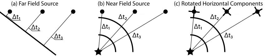
which is correlated with the observed data. Hence, it estimates the power contributions of plane waves in the data. The vectorrnpoints from thenth station to a reference point (usually one of the stations). A schematic
Figure 1.(a) The common assumption of plane wave beamforming, where a plane wave approaches the array. (b) Equivalent schematic example of a near-field source or arbitrary wave form and (c) the rotation of horizontal component required for three-component matched field processing. The wave front of the source-induced signal is displayed as the thick black line, raypaths as thin black lines, black dots as receivers, and the black stars as sources.
power of the signal. To account for this possibility one can reformulate the steering vector to be dependent on travel times instead of the slowness and sensor location
aqn(t) =e−2𝜋iftqn, (3)
wheretqnis the travel time between sourceqand receivernand illustrated in Figure 1. If the source is far away,
the wave front passes over the array as a (nearly) straight line and is equivalent to the previously discussed plane wave steering vector. With this modification, the beamforming process samples the power contribution of spatial locations. If we consider a single-component beamformer, this change alone would be sufficient to estimate near-field contributions. For the three-component case, where horizontal components are of inter-est, it is required to rotate the horizontal components into the direction of the back azimuth of the source (one horizontal direction looks toward the back azimuth of source, while the other is perpendicular) as shown in Figure 1c. This is common practice in the simplest three-component beamforming approaches where the horizontal components are rotated by an angle to estimate a far-field source (e.g., Haubrich & McCamy, 1969). In the case of a near-field source, each receiver is required to be rotated by an individual angle (see Figure 1c) for one specific source location.
We choose the three-component beamformer proposed by Wagner (1996) for our study. It has the advantage over the conventional approach (Haubrich & McCamy, 1969) in that it takes coherent polarization propagation into account, that is, power is estimated by means of coherent phase and polarization summation. We first give a brief introduction to the underlying equations, followed by the necessary modifications for the MFP case. The three-component data vector (of 3Kdimension) can be written as
x3C(t) = [
xZ(t),xN(t),xE(t) ]T
(4)
and the three-component cross-spectral density matrix (CSDM) can be calculated from its Fourier transformed partX3C(f)as
R3C(f) =X3C(f)XH
3C(f). (5)
The CSDM is a 3Kby 3KHermitian matrix, whereKis the number of stations. From here one can obtain the 3 by 3 polarization covariance matrix
Y3C(s,f) =eH(s,f)R3C(f)e(s,f) (6)
whereeis the orthogonal steering matrix
e(s,f) =
⎡ ⎢ ⎢ ⎣
a1,Z … aK,Z 0 … 0 0 … 0
0 … 0 a1,N … aK,N 0 … 0 0 … 0 0 … 0 a1,E … aK,E
⎤ ⎥ ⎥ ⎦ T
. (7)
on all components. An eigenvalue decomposition can be used to determine the principal components of this matrix, which in this case are the polarization states of the analyzed wavefield. The eigenvalues𝜆idetermine the power contribution of a certain polarization which is given by the corresponding eigenvectorsui(s,f). The power of the signal with the strongest polarization, which is determined by the corresponding eigenvector u0(s,f)of the largest eigenvalue𝜆0, is given as
⎡ ⎢ ⎢ ⎣
PZ(s,f)
PN(s,f)
PE(s,f) ⎤ ⎥ ⎥ ⎦ = ⎡ ⎢ ⎢ ⎣
|u0Z(s,f)|2 |u0N(s,f)|2 |u0E(s,f)|2 ⎤ ⎥ ⎥ ⎦𝜆0.
(8)
The power for the radial and transverse component can be obtained by rotating the horizontal components of the eigenvector into the desired direction
[
uR
uT ]
=M(𝛼)
[ uN uE ] = [
cos𝛼 sin𝛼
−sin𝛼 cos𝛼
] [
uN
uE ]
, (9)
where𝛼is the angle by which the components are rotated. More detail with regard to the beamformer can be found in Gal et al. (2016).
The extension to the MFP approach requires, as a first step, the rotation of the horizontal traces toward the direction of the source (north component pointing toward the source, which automatically will make it the radial component) following the illustration in Figure 1c and can be accomplished by the rotational matrixM, whereas the direction of the source is obtained from the raypaths calculated via fast marching. The rotated radial and transverse components are then placed into the data vector defined in equation (4) substitut-ing the north-south and east-west component. The rotated data vector is then used to compute the CSDM as in equation (5). A final modification is to replace the plane wave steering vectors in the steering matrix (equation (7)) with the fast marching travel time guided vectors from equation (3). The MFP steering matrix for theqth source is then
eq(s,f) =
⎡ ⎢ ⎢ ⎣
aq1,Z … aqK,Z 0 … 0 0 … 0
0 … 0 aq1,N … aqK,N 0 … 0
0 … 0 0 … 0 aq1,E … aqK,E ⎤ ⎥ ⎥ ⎦ T . (10)
For vertical and radial steering vectors we use the travel times derived from a Rayleigh wave phase velocity map, while for the transverse component we use the ones derived from a Love wave map. The beam power obtained for theqth source is in this case already in vertical, radial, and transverse coordinates and does not require additional rotation
⎡ ⎢ ⎢ ⎣
Pq,Z(f)
Pq,R(f)
Pq,T(f)
⎤ ⎥ ⎥ ⎦ = ⎡ ⎢ ⎢ ⎣
|u0,qZ(f)|2
|u0,qR(f)|2
|u0,qTf)|2
⎤ ⎥ ⎥ ⎦𝜆0.
(11)
2.2. Synthetic Test
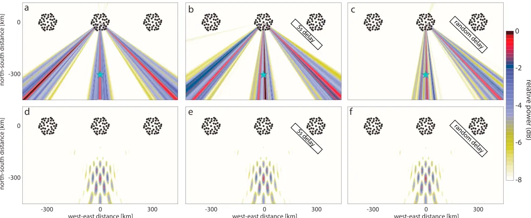
The synthetic test presented here is designed to demonstrate how plane wave beamforming behaves in con-ditions that strongly deviate from the plane wave assumption and how MFP is not bound by these restrictions. The test is carried out for single-component beamforming as the three-component case follows a similar logic. The synthetic array configuration is shown in Figure 2. The array is composed of three clusters, where the centers are 300 km apart. A synthetic point source is placed 300 km to the south off the middle cluster. We generate seismic traces of 800-s length at each receiver asxn(t) =cos(2𝜋f(tn+ Δt)), wheretnis the travel time
between thenth receiver and synthetic source, andΔtdenotes a travel time delay and use them as the input for our synthetic tests.
Figure 2.Synthetic tests which demonstrate the characteristics of plane wave beamforming (a–c) under conditions that violate the underlying propagation assumptions and matched field processing (d–f ), which accounts for arbitrary wave front geometries and their associated delay times (e,f ). Receivers are shown as black dots and the synthetic source as a blue star.
The resulting beam power for the plane wave approach is shown in Figure 2a. The approach identifies three back azimuths with increased beam power which are 135∘, 180∘, and 225∘. They are a direct result of the near-field source, where the curved wave front approaches each cluster with a differing back azimuth. It is clear in this example where the source location is known, that the power estimated at 135∘is due to the left cluster while the power estimated at 225∘is due to the right cluster. Hence, it is important to keep in mind that plane wave beamforming estimates power at back azimuths where partial plane wave coherence over an array area is given. Without the knowledge of the synthetic source location, this result might be misinterpreted as three equally strong far-field sources. An option would be to analyze each cluster on its own and infer the true source location, which in this synthetic case where the clusters are spatial separated is an easy task. In real-world array analysis, finding the spatially coherent parts of an array would involve many permutations on smaller subarrays to identify which combination of stations estimate a coherent wavefield. In addition to the above complications, the estimated power from the plane wave approach is∼0.16 which is roughly a factor of 6 lower than the true source power which was set as 1.
To simulate path propagation effects caused by a slow-velocity zone, we delay the phases of the right clus-ter by 5 s (Figure 2b). Even though the individual clusclus-ters are still relatively coherent, the overall resolution slightly degrades and a delay for one cluster affects the resolution of the remaining two. In the extreme case where phase delays for each station of the right cluster are assigned randomly (e.g., a large aperture array with strongly varying phase velocity), there is little power estimated at 225∘(Figure 2c), but a reduction of the remaining beam power is still visible.
In the case of MFP for the near-field source (Figure 2d), the source location and power are accurately esti-mated. Apart from the global beam power maximum, we see multiple local maxima in close proximity to the true source location, which are a result of imperfect spatial sampling given by the array configuration, appar-ent seismic velocity, and the chosen frequency. For the case of a 5-s and random delay (Figures 2e and 2f ), MFP obtains the same solution since we can account for the delays and do not have to follow a plane wave model. In real-world applications, where the phase delays are induced by velocity heterogeneities of the seis-mic propagation medium and they are accurately known (e.g., through a fast marching estimation of phase velocity maps), more precise estimate of source power and location will be obtained.
3. Data and Preliminary Testing
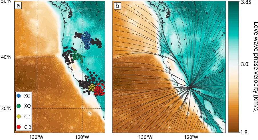
Figure 3.(a) Study area with four seismic networks where we use only the colored stations (blue = part of XC network; green = part of FAME array; yellow = part of SCSN; and red = combination of ANZA and SCSN). As the background, the Love wave phase velocity map at 8 s is shown, where the offshore regions are interpolated into the constant velocity of 3.2 km/s. (b) Raypaths for a single receiver in the center of CI1 and multiple sources distributed at the edges of the study area. It demonstrates path propagation effects due to velocity heterogeneities calculated with fast marching. XC = High Lava Plains Broadband Seismic Experiment; FAME = Mendocino Experiment-EarthScope Flex Array; SCSN = Southern California Seismic Network; ANZA = ANZA regional network.
A well-studied area is chosen, where phase velocity maps for Rayleigh and Love waves in the desired frequency range exist and a seismic array for the intended task is available. Fast marching (Rawlinson & Sambridge, 2005) is applied to the Rayleigh and Love phase velocity maps to calculate travel times and bearing angles (back azimuth between all source-receiver pairs that account for velocity heterogenities) on a source-receiver grid. The calculated travel times and bearing angles are used as input parameters to steer the three-component beamformer (Wagner, 1996).
3.1. Area and Phase Velocity Maps
A suitable area for our study is the west coast of the United States, which has been subject of multiple seismic-phase velocity tomography studies (e.g., Ekström, 2014; Lin et al., 2009; Shen & Ritzwoller, 2016) and hosts a range of seismic networks which can be utilized to study microseisms. As the underlying Rayleigh and Love phase velocity maps, we use the results from the eikonal tomography at 8 and 16 s generated by Lin et al. (2009), which cover the peak period range of primary and secondary microseisms.
The phase velocity maps cover the majority of the United States but need to be extended to cover the ocean areas where microseisms are generated. For primary microseisms (16 s) this is achieved by smoothly interpo-lating the velocity map edges into a constant value. All original values of the eikonal tomography are retained and a smooth transition toward missing values is achieved. At 16 s the interpolation velocities are 3.7 km/s and 3.5 km/s for Love and Rayleigh waves, respectively. The values are chosen as a compromise to minimize the velocity gradient toward the edges of the original tomography map. This approximation using an empirical offshore velocity is justified for primary microseims where little velocity difference between land and offshore regions was observed (Bowden et al., 2016). Additionally, raypaths from the seismic array converge toward a source, and hence, all raypaths between the source and receivers are likely to experience the same velocity heterogeneities in the oceanic environment, which can be approximated with a constant velocity. The pre-cise velocity offshore does not have to be known, as the beamformer depends on the time delays between stations and not on the actual travel time.
with Bowden et al., 2016) and an example of the Love wave phase velocity map is shown in Figure 3a. Rayleigh and Love wave maps at 8 s are constructed in a two-stage approach. First, the respective tomography maps at 8 s are extended by a constant velocity on land where no phase velocity is defined (Rayleigh = 3.05 km/s and Love = 3.2 km/s) and smoothed toward the original tomography map in order to remove discontinuities.
In a second step the velocity in offshore regions is calculated as
v(x,y) =vc−
d(x,y)
4,000, (12)
wherevcis the 3.05 and 3.2 km/s for Rayleigh and Love waves, respectively, andd(x,y)is the spatially depen-dent bathymetry in meters withxandybeing the spatial coordinates. The right-hand side term reduces the velocity linearly with depth and at 4-km depth the velocity is reduced by 1 km/s, which yields the observed Rayleigh wave phase velocity (Bowden et al., 2016). Love waves are assumed to be roughly 9% faster (Lin et al., 2009), which is in agreement with the above equation.
3.2. Seismic Arrays
The west coast of the United States offers a wide range of seismic arrays (temporary and permanent). The choice of array for this study is based on maximizing the spatial coverage at a given time period which involves a suitable time overlap of operating permanent and temporary networks (early 2009 is found to be suitable). The four arrays are the Southern California Seismic Network (SCSN; California Institute of Technology (Caltech), C. I., 1926), the ANZA regional network (ANZA; Vernon & Diego, 1982), the High Lava Plains Broadband Seis-mic Experiment (XC; James & Fouch, 2006), and the Mendocino Experiment - EarthScope Flex Array (FAME; Levander, 2007). Only parts of some arrays are suitable given their operational time period or data availability, and all stations are shown in Figure 3a. We use only parts of the available arrays to either prevent overestima-tion of certain direcoverestima-tions due to the array configuraoverestima-tion (e.g., FAME array) or to prevent near-coastal staoverestima-tions from entering the MFP procedure, which has been shown to degrade the beam power in preliminary test-ing. Four arrays are formed and denoted as CI1, CI2, XC, and XQ where CI1 is part of SCSN, CI2 is part of SCSN and ANZA, XC is part of the High Lava Plains Broadband Seismic Experiment, and XQ is part of FAME (for more details see Figure 3a). All of these arrays have three-component sensors and instruments that have a flat response (LHZ/N/E) in the microseism range.
3.3. Source-Receiver Grid and Path Effect Parameters
The source grid is constructed between 135–115∘W longitude and 25–50∘N latitude. The area is discretized into a 0.25∘by 0.25∘source grid, which was chosen as a compromise between computational burden and suf-ficient resolution. The source-receiver grid is then constructed as a permutation between all source-receiver pairs.
The source-receiver grid in combination with the phase velocity maps is used as the input for the fast marching method (Rawlinson & Sambridge, 2005), which is a grid-based eikonal solver that tracks first-arriving wave fronts. For each source-receiver pair, a synthetic circular wave front is simulated that progressively evolves outward from the source. The synthetic wave front will be distorted by the seismic velocity heterogeneities of the phase velocity map, and hence accounts for travel time deviations from a constant velocity model and wave front bending, that is, propagation path effects. An example is shown in Figure 3b, where raypaths for a single receiver are shown for 180 sources placed at the edges of our study area. The output that we require from the fast marching approach are the travel times and bearing angles for each source-receiver pair.
3.4. Seismic Data and Processing
If a receiver has a median power that is larger or smaller by a factor of 20 on any specific day, the receiver is excluded from any further calculation.
We use the travel times and bearing angles obtained at an earlier stage from fast marching as input parameters for MFP. For each source pointqthe observed data vector is rotated to form a radial and transverse component
⎡ ⎢ ⎢ ⎣
xZ(t)
xR,q(t)
xT,q(t)
⎤ ⎥ ⎥ ⎦←
−M(𝛼q)←−
⎡ ⎢ ⎢ ⎣
xZ(t)
xN(t)
xE(t)
⎤ ⎥ ⎥ ⎦.
(13)
This will ensure that for a given source the polarization at all receivers will be coherent as long as the prop-agation model is accurately estimated. Unlike in plane wave beamforming where the rotation angle𝛼 is identical for all stations, in MFP𝛼is determined by fast marching and is likely to differ for all stations. Addi-tionally we modify the steering matrixe, where travel times derived from fast marching are inserted for each source-receiver pair as shown in equation (10).
The data, sampled at 1 Hz, are cut into 800-s-long windows with 50% overlap. In contrast to plane wave beam-forming, a well-resolved frequency spectrum is of higher importance to guarantee accurate coherent phase summation. In plane wave beamforming, inaccuracies in the spectral estimation lead to a bias in the appar-ent slowness estimation. In MFP, where the phase velocity of the propagation medium is predefined, a poorly estimated frequency spectrum results in a degradation of beam power, and hence an inaccurate represen-tation of the observed wavefield. With decreasing frequency, this effect become less important (wavelength increases and a deviation from the predicted travel time has a smaller effect on phase), and hence, we use the same window length for the primary microseism analysis as well.
Each window is tapered by the Hann window function to reduce spectral leakage and rotated into the direc-tion of the source before applying the Fourier transform. Each spectral windowiis normalized by the total power of all three components
̃
Xi,3C(f) =
Xi,3C(f)
Li
with Li= √
||Xi,Z(f)||
2
+||Xi,R(f)||
2
+||Xi,T(f)||
2
. (14)
This is especially important for seismic arrays with large apertures to reduce spurious amplitude features induced by, for example, earthquakes, path propagation effects, and sensor faults. The CSDM is then averaged over time to obtain an average daily representation of the wavefield
R3C(f) =
1 N
∑
i ̃
Xi,3C(f)X̃Hi,3C(f), (15)
whereNis the number of windows.
For our MFP approach we chose the frequency wave number (f-k) approach as the underlying beamformer. We have tested higher-resolution algorithms such as MVDR (Capon, 1969) and MUSIC (Schmidt, 1986) but did not find any significant performance increase when analyzing fundamental Rayleigh and Love waves. This is likely due to the robust nature of the f-k approach, while MVRD and MUSIC have stronger penalization in the case of a synthetic versus observed field phase mismatch. With higher-quality-phase velocity maps, the higher-resolution approaches are likely to become the preferred methods in the future.
3.5. Sensitivity of the Approach
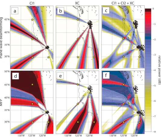
Figure 4.Resolution and sensitivity tests using four synthetic sources (yellow stars) for plane wave beamforming (top row) and MFP (bottom row). The sensitivity is demonstrated with the CI1 array (a, d), the XC array (b, e), and an incoherently combined result of CI1+CI2+XC (c, f ). We used travel times obtained with fast marching from the 8-s Rayleigh wave map to generate the synthetic data. Sensitivity maps for Love waves follow a similar pattern. MFP = matched field processing; XC = High Lava Plains Broadband Seismic Experiment.
Figure 5.Analysis of the Chino Hills earthquake in California with a part of the SCSN (a, b) and XC (c, d). Results from plane wave beamforming (left column) and MFP (right column) are shown. The true earthquake location is marked by the two red circles. SCSN = Southern California Seismic Network; XC = High Lava Plains Broadband Seismic Experiment; MFP = matched field processing.
3.6. Earthquake Source
To verify the applicability of our approach to observed data, we analyze the Chino Hills earthquake (magnitude 5.5Mw) which occurred in Southern California on 29 July 2008. The earthquake is analyzed with the available
This simple test shows that the radial resolution (radial-outgoing from the array center) is poorer than the perpendicular resolution, which can be explained by the bearing angles. A virtual source that is moved away from the array will induce strong bearing angle changes in the near field that asymptotically diminish with increasing source-array distance until the far-field approximation is reached. Hence, the farther the source is away from the array, the less accurate it can be constrained in distance. This manifests as streaks of beam power in the radial direction. In MFP, this is addressed by a modification of the steering vector to weaken beam power with distance. While this modification is useful for the very near field case and point sources, it does not perform well at our scales and is therefore not implemented. If used, it would lead to an over amplification of the near field given that multiple sources with differing azimuths are present in the microseism wavefield.
Ideally we would like to use all available seismic stations simultaneously to increase the radial resolution. For the example of an earthquake, this is possible since the earthquake can be approximated by a single point source with a well-defined signal onset. The spectral properties of the observed wavefield at each station are representative of the earthquake source, and phase coherent summation will be applicable. For microseisms the sources are spatially extended and while they can be modeled as a superposition of multiple point sources, the resulting wavefield is dependent on the spatial distribution of the individual point sources and their indi-vidual source function. Hence, the spectral phases calculated from the observed wavefield are modified for each propagation direction and coherent summation is unlikely to succeed. An example demonstrating the issue with a coherent summation for two point sources is displayed in Figure S3. We therefore chose to ana-lyze microseisms separately by each seismic array and incoherently average the resulting normalized beam powers.
Additionally, we process an offshore earthquake with conventional plane wave f-k beamforming and MFP to estimate the accuracy of our approach for the offshore environment (Figure S2) at 8 s where we use the depth-dependent phase velocity. The earthquake epicenter is accurately located with our MFP approach using Rayleigh and Love waves, and hence validates the accuracy of our approach.
4. Results
4.1. Primary Microseims
The combined beam power maps from MFP for the three days are shown in Figure 6. For each day, we display the ocean wave height and dominant swell direction (Figures 6a, 6d, and 6g) for a comparison with the com-bined beam power maps from all four arrays. For completeness, all the results from each array are displayed in the supporting information (Figure S4–S6). The beam power in deeper parts of the ocean was empirically reduced given that the effective excitation of 16 s primary microseisms is distributed around a depth of 30 m (Ardhuin et al., 2015). We observe that primary microseisms do not show significant spatial changes in the combined result even though the spatial swell distribution and wave height differ on all three days. The wave heights do not correlate with the relative beam powers, which point toward the same areas for all three days. This is not surprising since the transfer of swell energy to primary microseism is bathymetry and sea bottom slope dependent (for bathymetry information, see Figure S7). The areas where bathymetry and slope config-uration are favorable show the highest beam power. The southwestern coast line of Vancouver Island with many shallow continental shelf regions generates the strongest Rayleigh and Love waves. Additionally, the island’s coastline is in line with the seismic arrays, and hence the power contribution from sources are added constructively to increase the power.
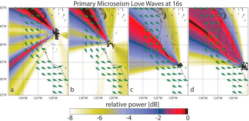
Figure 7.Detailed beam maps from all four arrays for primary microseisms on 28 March. The green arrows denote the mean swell direction as in Figure 6.
The two remaining arrays (Figures 7c and 7d) also observe Love waves which could originate from the same source. If they originate from the same coastline, it would be in violation of the assumed directional radiation. However, it is not clear whether they are generated in the same place. They could be generated farther down the coast which faces west. Given that both CI1 and CI2 observe primary microseism Rayleigh waves from the south west (Figure S6a and S6b) while no Love waves are detected (Figures S6e and S6f ), the generation mechanism proposed by Saito (2010) appears to be valid.
Another striking feature is the difference in beam power maps between the two arrays in Figures 7c and 7d. The centers of the two arrays are only∼200 km apart, but CI1 observes only weak energy from Vancouver Island compared to CI2. This example shows that path propagation effects can strongly influence the observed wavefield even within a few hundred kilometers.
We estimate the Rayleigh to Love wave ratio from the radial to transverse component between the strongest primary microseism sources for each day (only beam power from oceanic grid points is counted). The ratios are XC 0.7±0.02, XQ 0.35±0.08, CI1 0.3±0.03, and CI2 0.32±0.06. They were estimated as the mean from the three days of data used for analysis along with their respective standard deviations used as confidence inter-vals. This is in accordance with previous studies which show that Love waves dominate the primary microseism range (e.g., Nishida et al., 2008).
4.2. Secondary Microseisms
Secondary microseisms are not generated by direct coupling between ocean waves and the solid Earth, but require second-order ocean gravity wave pressure fluctuations that are created by two swell trains with similar frequency and opposite direction. The IFREMER model is capable of hindcasting these pressure fluctuations, which excite secondary microseisms. Hence, instead of using wave heights to gauge the source regions we utilize the model-predicted pressure fluctuations to calculate the displacement as seen from each array and combine it to obtain an average result which is displayed in Figures 8a, 8d, and 8g for the three days. We use the hindcast with coastal reflection coefficients of 10/20/40% for resolved land (anything bigger than 0.5∘), unresolved land (smaller than 0.5∘) and icebergs. Additionally, we use the ocean site effects as given by Longuet-Higgins (1950). For the attenuation term, we choose a group velocityvg = 2.6km/s and a quality factorQ=150. While the group velocity is a realistic value in our region, the quality factor is chosen empir-ically. We used previously estimated products ofvgQ(Stutzmann et al., 2012) as a guideline for the bounds
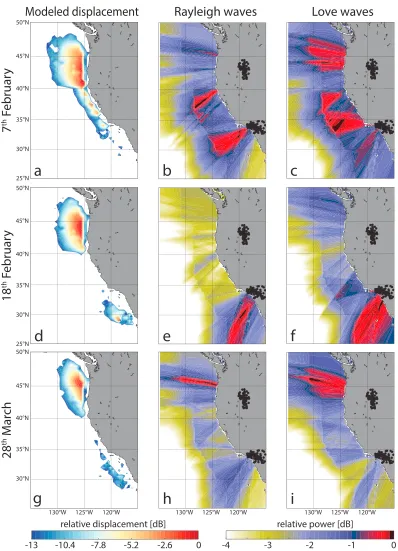
Figure 8.Combined results for secondary microseisms following the same outline as Figure 5, with the exception of the first column which replaces wave heights by displacement associated with secondary microseism excitation.
CI1 and CI2 first, normalize the beam map, and then average with XC to produce the final result displayed in Figure 8. The beam map cutoff boundary in deeper ocean is extended to account for reasonable distances aided by the predicted displacements from the IFREMER model. This is a reasonable assumption given that displacement contributions from regions farther from the coast are predicted to be negligible (see Figures 8a, 8d, and 8g).
The observed source regions correlate well with the model-predicted regions with the exception of the 40∘N–45∘N/130∘W–125∘W quadrant where strong displacement is predicted but not observed. The general trend shows that Rayleigh and Love wave generation regions are closely related; however, the beam map reveals differences as well. On 7 February (Figures 8a–8c) differences offshore of California are visible between Rayleigh and Love waves. The same spatial region is also more pronounced for Love waves on 18 February.
A good opportunity to study the differences between Rayleigh and Love waves is identified on 18 February, where a strong and spatially constrained source is predicted by the model (Figure 8d). The observed Rayleigh waves are estimated from the expected region and match the model well. For Love waves the estimated source region is broader and around the Rayleigh wave source maximum. A similar but less pronounced pat-tern can be found on 28 March where Love wave maxima are distributed around the Rayleigh wave source region.
The Rayleigh to Love wave ratios, calculated between the strongest source in the ocean of the radial and transverse component, are XC 0.86±0.13, CI1 1.28±0.14 and CI2 1.24±0.19. Hence, the southern arrays show a dominance toward Rayleigh waves and the northern array shows a slightly higher Love wave power distribution between the horizontal components of Love and Rayleigh waves.
5. Discussion
The following section is divided into the discussion of the technique and the results. We discuss the optimal way MFP can be applied to the observation of microseisms and possible ongoing developments. Then, we discuss the differences between the ocean hindcast and the observed wavefield, differences between source regions of Rayleigh and Love waves and their ratios, and potential Love wave generation mechanisms.
We observe in our study that MFP of surface wave microseisms works best if the seismic array location is not in the immediate near field of extended sources. This is directly linked to the spatial extent of the source area and the resulting frequency spectrum which yields an average phase of the source. The ill-conditioned Fourier spectrum is likely to degrade the performance of the beamformer and might lead to beam power estimates with low confidence. This problem could be addressed by spatial averaging to decorrelate the spatial source with the help of a very dense uniform linear array (Goldstein & Archuleta, 1991). Another option to increase confidence in the results is to use arrays with a large number of sensors. With an increasing number of sen-sors a better estimate of the spatial Fourier spectrum can be achieved. We have experimented with different temporal windows lengths (200–8,000 s) but have found little difference in the results. While a large window will give a better Fourier spectrum estimation, more sources are present in the estimated seismic trace. By contrast, a short trace will have less sources but a poorer frequency resolution.
Another factor for the accurate estimation of the wavefield are the phase velocity maps. They are currently at a precision where f-k MFP yields consistent results that correlate well with a hindcast. In the future, where new or improved phase velocity maps will be generated for more regions, the access to MFP will potentially allow higher-resolution techniques to be applied. With the deployment of OBS stations, the phase velocity cover-age of offshore regions will be extended and allow for better source location of microseism surface waves. Additionally, one could substitute the fast marching method with a finite difference or finite element method for solving the full elastic wave equation in order to account for finite frequency effects in the propagation medium. This will be especially beneficial for local models where the seismic structure is well constrained and amplitude sensitive MFP will be available. On the other hand, the current approach with fast marching is sev-eral orders of magnitude faster in terms of computational time (travel times and bearing angles for this study were calculated under an hour on a single CPU core).
of model errors and path propagation effects. We have tested different settings for the predicted microseism excitation (Ardhuin & Roland, 2012), which are wave height, period, and bottom slope of the shore face depen-dent and displayed the results in Figure S11, but found little difference which would explain the mismatch between model and observation. The observational absence for predictions of strong displacement from the 40∘N–45∘N/130∘W–125∘W quadrant (Figurea 8b, 8e, and 8h) could be due to increased sediment thickness (Divins, 2003; Wong & Grim, 2015) in the generation area, which has been shown to trap and successively reduce the microseism energy propagating toward the receiver (Gualtieri et al., 2015). Additionally, we have tried to analyze earthquake surface waves originating from this quadrant. We were not able to find any sur-face waves with the XC array for multiple earthquakes with a magnitude>5 mb. Hence, it is very likely that a large part of the energy from this region is blocked on its path to the array. For California the improved param-eterization of the microseismic displacement model (Ardhuin & Roland, 2012) shows an increase in modeled displacement in the southern regions (Figures S11c and S11d), which fits well for 18 February and 28 March but is absent on 7 February.
A general agreement between source regions of secondary microseism Rayleigh and Love waves is observed, but on a smaller scale differences are identified. Love waves whose generation mechanism in the secondary microseism range is to date unclear, have in the past been identified to originate from similar azimuths as Rayleigh waves (e.g., Haubrich & McCamy, 1969; Lacoss et al., 1969); however, a recent high-resolution study showed that the azimuths can differ (Gal et al., 2017). With the current study we are able to estimate the generation regions with the help of multiple arrays and can further constrain the potential generation mechanisms.
A suggested conversion from oceanic Rayleigh waves to continental Love waves (Gregersen, 1978) seems unlikely to be a major contributor. The conversion is predicted to be more important with an increasing seabed slope and long wavelength of Rayleigh waves. Such conversion for primary microseisms is on multiple occa-sions not observed (Figures S4b, S4c, S4f, S4g, S5a, S5c, S5e, S5g, S6a, S6b, S6e, and S6f ), and hence, it is unlikely that it would have a significant effect in the secondary microseism range. The only exceptions are arrays XQ and XC, which observe Rayleigh and Love waves from the direction of Vancouver Island, but the continental slope in this region is very small and hence it is unlikely that a conversion takes place. Further, a proposed excitation via seamounts would require the generation regions to be identical or at least confined within the generation areas of Rayleigh waves. This type of generation is not observed for Love waves which seem to originate from a broader region than Rayleigh waves.
Other proposed excitations are via a type of scattering or interaction with a sedimentary basin. Of these two scenarios, scattering from Rayleigh to Love waves seems to be the more likely mechanism, as Rayleigh waves radiate from the source omnidirectionally and scattering into Love waves during their propagation would create a larger source area for Love waves. An interesting observation is that Love wave source maxima seem to lie around that of Rayleigh waves (Figures 8e, 8f, 8h, and 8i). A similar observation has been observed for SH waves by Liu et al. (2016) in their Figure 5d, which could point to a similar excitation for Love and SH waves.
The energy ratio between Rayleigh and Love waves has been under increasing investigation in recent years (e.g., Gal et al., 2017; Juretzek & Hadziioannou, 2016; Nishida et al., 2008; Tanimoto et al., 2015, 2016). Our observations confirm prior findings that Love waves are stronger in the primary microseism range and equal or weaker on average in the secondary microseism range. The ratios depend on the geographical location (Juretzek & Hadziioannou, 2016) and also differ in back azimuth for the respective array (Gal et al., 2017). In this study we find that different source locations result in different Rayleigh to Love wave ratios, and hence, the ratio is a function of source location, path propagation effects, and geographical position of the array. Given that secondary microseism source locations change with time, the Rayleigh-Love wave ratio also varies with time.
6. Conclusions
When applied to the microseism wavefield in the western United States, we find primary microseisms to be dominated by Love waves, which show directional characteristics as predicted by theory. In the secondary microseism range, Rayleigh waves are on average equal or stronger to Love waves and both originate from similar regions. On smaller scales, a difference between the generation regions is observed, where Love waves show excitation in a broader area compared to Rayleigh waves. The most likely excitation mechanism of Love waves seems to be scattering from Rayleigh to Love waves. We observe a pattern where source maxima of Love waves lie around the source maxima of Rayleigh waves, which agrees with the pattern of previously observed secondary microseism SH waves located around thePwave source.
References
Ardhuin, F., Gualtieri, L., & Stutzmann, E. (2015). How ocean waves rock the Earth: Two mechanisms explain microseisms with periods 3 to 300 s.Geophysical Research Letters,42, 765–772. https://doi.org/10.1002/2014GL062782.1
Ardhuin, F., & Roland, A. (2012). Coastal wave reflection, directional spread, and seismoacoustic noise sources.Journal of Geophysical Research,117, C00J20. https://doi.org/10.1029/2011JC007832
Ardhuin, F., Stutzmann, E., Schimmel, M., & Mangeney, A. (2011). Ocean wave sources of seismic noise.Journal of Geophysical Research,116, C09004. https://doi.org/10.1029/2011JC006952
Baggeroer, A., Kuperman, W., & Mikhalevsky, P. (1993). An overview of matched field methods in ocean acoustics.IEEE Journal of Oceanic Engineering,18(4), 401–424. https://doi.org/10.1109/48.262292
Baggeroer, A., Kuperman, W. A., & Schmidt, H. (1988). Matched field processing: Source localization in correlated noise as an optimum parameter estimation problem.Journal of the Acoustic Society of America,83, 571–587.
Behr, Y., Townend, J., Bowen, M., Carter, L., Gorman, R., Brooks, L., & Bannister, S. (2013). Source directionality of ambient seismic noise inferred from three-component beamforming.Journal of Geophysical Research: Solid Earth,118, 240–248. https://doi.org/10.1029/2012JB009382
Beyreuther, M., Barsch, R., Krischer, L., Megies, T., Behr, Y., & Wassermann, J. (2010). Obspy: A Python toolbox for seismology.Seismological Research Letters,81(3), 530–533. https://doi.org/10.1785/gssrl.81.3.530
Boue, P., Poli, P., Campillo, M., Pedersen, H., Briand, X., & Roux, P. (2013). Teleseismic correlations of ambient seismic noise for deep global imaging of the Earth.Geophysical Journal International,194(2), 844–848. https://doi.org/10.1093/gji/ggt160
Bowden, D. C., Kohler, M. D., Tsai, V. C., & Weeraratne, D. S. (2016). Offshore Southern California lithospheric velocity structure from noise cross-correlation functions.Journal of Geophysical Research: Solid Earth,121, 3415–3427. https://doi.org/10.1002/2016JB012919 Bromirski, P., & Duennebier, F. (2002). The near-coastal microseism spectrum: Spatial and temporal wave climate relationships.Journal of
Geophysical Research,107(B8), 2166. https://doi.org/10.1029/2001JB000265
Bromirski, P. D., Duennebier, F. K., & Stephen, R. A. (2005). Mid-ocean microseisms.Geochemistry, Geophysics, Geosystems,6, Q04009. https://doi.org/10.1029/2004GC000768
Bromirski, P. D., Stephen, R. A., & Gerstoft, P. (2013). Are deep-ocean-generated surface-wave microseisms observed on land?Journal of Geophysical Research: Solid Earth,118, 3610–3629. https://doi.org/10.1002/jgrb.50268
Brooks, L., Townend, J., Gerstoft, P., Bannister, S., & Carter, L. (2009). Fundamental and higher-mode Rayleigh wave characteristics of ambient seismic noise in New Zealand.Geophysical Research Letters,36, L23303. https://doi.org/10.1029/2009GL040434
Bucker, H. (1976). Use of calculated sound fields and matched-field detection to locate sound sources in shallow-water.The Journal of the Acoustical Society of America,59(2), 368–373. https://doi.org/10.1121/1.380872
California Institute of Technology (Caltech), C. I. (1926). Southern California Seismic Network. International Federation of Digital Seismo-graph Networks. Other/Seismic Network. https://doi.org/10.7914/SN/CI
Capon, J. (1969). High-resolution frequency-wavenumber spectrum analysis.Proceedings of the IEEE,57(8), 1408–1418. https://doi.org/10.1109/PROC.1969.7278
Capon, J. (1973). Analysis of microseismic noise at LASA, NORSAR and ALPA.Geophysical Journal of the Royal Astronomical Society,35, 39–54.
Cessaro, R. K. (1994). Sources of primary and secondary microseisms.Bulletin of the Seismological Society of America,84(1), 142–148. Chevrot, S., Sylvander, M., Benahmed, S., Ponsolles, C., Lefèvre, J. M., & Paradis, D. (2007). Source locations of secondary
micro-seisms in western Europe: Evidence for both coastal and pelagic sources.Journal of Geophysical Research,112, B11301. https://doi.org/10.1029/2007JB005059
Corciulo, M., Roux, P., Campillo, M., Dubucq, D., & Kuperman, W. A. (2012). Multiscale matched-field processing for noise-source localization in exploration geophysics.Geophysics,77(5), KS33–KS41. https://doi.org/10.1190/geo2011-0438.1
Cros, E., Roux, P., Vandemeulebrouck, J., & Kedar, S. (2011). Locating hydrothermal acoustic sources at old faithful geyser using matched field processing.Geophysical Journal International,187(1), 385–393. https://doi.org/10.1111/j.1365-246X.2011.05147.x
Divins, D. (2003). Total sediment thickness of the world’s oceans & marginal seas. NOAA National Geophysical Data Center, Boulder, CO, (Viewed 08 February 2017). Retrieved from https://www.ngdc.noaa.gov/mgg/sedthick/sedthick.html
Ekström, G. (2014). Love and Rayleigh phase-velocity maps, 5–40 s, of the western and central USA from USArray data.Earth and Planetary Science Letters,402, 42–49. https://doi.org/https://doi.org/10.1016/j.epsl.2013.11.022
Euler, G. G., Wiens, D., & Nyblade, A. A. (2014). Evidence for bathymetric control on the distribution of body wave microseism sources from temporary seismic arrays in Africa.Geophysical Journal International,197(3), 1869–1883. https://doi.org/10.1093/gji/ggu105
Farra, V., Stutzmann, E., Gualtieri, L., Schimmel, M., & Ardhuin, F. (2016). Ray-theoretical modeling of secondary microseismPwaves.
Geophysical Journal International,206(3), 1730–1739. https://doi.org/10.1093/gji/ggw242
Friedrich, A., Klinge, K., & Krüger, F. (1998). Ocean-generated microseismic noise located with the Graefenberg array.Journal of Seismology,
2(1), 47–64.
Gal, M., Reading, A. M., Ellingsen, S. P., Gualtieri, L., Koper, K. D., Burlacu, R., & Tkalˇci´c, H. (2015). The frequency dependence and loca-tions of short-period microseisms generated in the Southern Ocean and West Pacific.Journal of Geophysical Research: Solid Earth,120, 5764–5781. https://doi.org/10.1002/2015JB012210
Gal, M., Reading, A. M., Ellingsen, S. P., Koper, K. D., & Burlacu, R. (2017). Full wavefield decomposition of high-frequency secondary micro-seisms reveals distinct arrival azimuths for Rayleigh and Love waves.Journal of Geophysical Research: Solid Earth,122, 4660–4675. https://doi.org/10.1002/2017JB014141
Acknowledgments
Gal, M., Reading, A. M., Ellingsen, S., Koper, K. D., Burlacu, R., & Gibbons, S. J. (2016). Deconvolution enhanced direction of arrival estima-tion using one- and three-component seismic arrays applied to ocean induced microseisms.Geophysical Journal International,206(1), 345–359. https://doi.org/10.1093/gji/ggw150
Gerstoft, P., Shearer, P. M., Harmon, N., & Zhang, J. (2008). Global P, PP, and PKP wave microseisms observed from distant storms.Geophysical Research Letters,35, L23306. https://doi.org/10.1029/2008GL036111
Goldstein, P., & Archuleta, R. J. (1991). Deterministic frequency-wavenumber methods and direct measurements of rupture propagation during earthquakes using a dense array: Theory and methods.Journal of Geophysical Research,96(B4), 6173–6185.
Gregersen, S. (1978). Possible mode conversion between Love and Rayleigh waves at a continental margin.Geophysical Journal of the Royal Astronomical Society,54(1), 121–127. https://doi.org/10.1111/j.1365-246X.1978.tb06759.x
Gualtieri, L., Stutzmann, E., Capdeville, Y., Farra, V., Mangeney, A., & Morelli, A. (2015). On the shaping factors of the secondary microseismic wavefield.Journal of Geophysical Research: Solid Earth,120, 6241–6262. https://doi.org/10.1002/2015JB012157
Gualtieri, L., Stutzmann, E., Farra, V., Capdeville, Y., Schimmel, M., Ardhuin, F., & Morelli, A. (2014). Modelling the ocean site effect on seismic noise body waves.Geophysical Journal International,197(2), 1096–1106. https://doi.org/10.1093/gji/ggu042
Hadziioannou, C., Gaebler, P., Schreiber, U., Wassermann, J., & Igel, H. (2012). Examining ambient noise using colocated measurements of rotational and translational motion.Journal of Seismology,16, 787–796. https://doi.org/10.1007/s10950-012-9288-5
Harris, D. B., & Kvaerna, T. (2010). Superresolution with seismic arrays using empirical matched field processing.Geophysical Journal International,182(3), 1455–1477. https://doi.org/10.1111/j.1365-246X.2010.04684.x
Hasselmann, K. (1963). A statistical analysis of the generation of microseisms.Reviews of Geophysics,1(2), 177–210. Haubrich, R. A., & McCamy, K. (1969). Microseisms: Coastal and pelagic sources.Reviews of Geophysics,7(3), 539–571.
Haubrich, R., Munk, W., & Snodgrass, F. (1963). Comparative spectra of microseisms and swell.Bulletin of the Seismological Society of America,
53(1), 27–37.
James, D., & Fouch, M. (2006). Collaborative research: Understanding the causes of continental intraplate tectonomagmatism: A case study in the Pacific Northwest. International Federation of Digital Seismograph Networks. Other/Seismic Network. https://doi.org/10.7914/SN/XC_2006
Juretzek, C., & Hadziioannou, C. (2016). Where do ocean microseisms come from? A study of Love-to-Rayleigh wave ratios.Journal of Geophysical Research: Solid Earth,121, 6741–6756. https://doi.org/10.1002/2016JB013017
Juretzek, C., & Hadziioannou, C. (2017). Linking source region and ocean wave parameters with the observed primary microseismic noise.
Geophysical Journal International,211(3), 1640–1654. https://doi.org/10.1093/gji/ggx388
Kedar, S., Longuet-Higgins, M., Webb, F., Graham, N., Clayton, R., & Jones, C. (2008). The origin of deep ocean microseisms in the North Atlantic Ocean, Proceedings of the Royal Society A: Mathematical.Physical and Engineering Sciences,464(2091), 777–793. https://doi.org/10.1098/rspa.2007.0277
Kelly, E. J. (1967). Response of seismic signals to wide-band signals. Lincoln Lab. Tech. Note, 30.
Kennett, B. (2005). Seismological tables: Ak135. Research School of Earth Sciences, The Australian National University, Australia.
Koper, K. D., de Foy, B., & Benz, H. (2009). Composition and variation of noise recorded at the Yellowknife Seismic Array, 1991–2007.Journal of Geophysical Research,114, B10310. https://doi.org/10.1029/2009JB006307
Koper, K. D., Seats, K., & Benz, H. (2010). On the composition of Earth’s short-period seismic noise field.Bulletin of the Seismological Society of America,100(2), 606–617. https://doi.org/10.1785/0120090120
Lacoss, R., Kelly, E., & Toksöz, M. (1969). Estimation of seismic noise structure using arrays.Geophysics,34(1), 21–38.
Landès, M., Hubans, F., Shapiro, N. M., Paul, A., & Campillo, M. (2010). Origin of deep ocean microseisms by using teleseismic body waves.
Journal of Geophysical Research,115, B05302. https://doi.org/10.1029/2009JB006918
Legaz, A., Revil, A., Roux, P., Vandemeulebrouck, J., Gouédard, P., Hurst, T., & Boléve, A. (2009). Self-potential and passive seismic monitoring of hydrothermal activity: A case study at Iodine Pool, Waimangu Geothermal Valley, New Zealand.Journal of Volcanology and Geothermal Research,179(1), 11–18. https://doi.org/10.1016/j.jvolgeores.2008.09.015
Levander, A. (2007). Seismic and geodetic investigations of Mendocino triple junction dynamics. International Federation of Digital Seismograph Networks. Other/Seismic Network. https://doi.org/10.7914/SN/XQ_2007
Lin, F.-C., Ritzwoller, M. H., & Snieder, R. (2009). Eikonal tomography: Surface wave tomography by phase front tracking across a regional broad-band seismic array.Geophysical Journal International,177(3), 1091–1110. https://doi.org/10.1111/j.1365-246X.2009.04105.x Liu, Q., Koper, K. D., Burlacu, R., Ni, S., Wang, F., Zou, C., et al. (2016). Source locations of teleseismic P, SV, and SH waves
observed in microseisms recorded by a large aperture seismic array in China.Earth and Planetary Science Letters,449, 39–47. https://doi.org/10.1016/j.epsl.2016.05.035
Longuet-Higgins, M. (1950). A theory of the origin of microseisms.Philosophical Transactions of the Royal Society of London. Series A. Mathematical and Physical Sciences,243(857), 1–35.
NCEDC (2014). Northern California earthquake data center. UC Berkeley Seismological Laboratory. Dataset. https://doi.org/10.7932/NCEDC Neale, J., Harmon, N., & Srokosz, M. (2017). Monitoring remote ocean waves using P-wave microseisms.Journal of Geophysical Research:
Oceans,122, 470–483. https://doi.org/10.1002/2016JC012183
Nishida, K., Kawakatsu, H., Fukao, Y., & Obara, K. (2008). Background Love and Rayleigh waves simultaneously generated at the Pacific Ocean floors.Geophysical Research Letters,35, L16307. https://doi.org/10.1029/2008GL034753
Nishida, K., & Takagi, R. (2016). Teleseismic S wave microseisms.Science,353(6302), 919–921. https://doi.org/10.1126/science.aaf7573 Obrebski, M. J., Ardhuin, F., Stutzmann, E., & Schimmel, M. (2012). How moderate sea states can generate loud seismic noise in the deep
ocean.Geophysical Research Letters,39, L11601. https://doi.org/10.1029/2012GL051896
Obrebski, M., Ardhuin, F., Stutzmann, E., & Schimmel, M. (2013). Detection of microseismic compressional (p) body waves aided by numeri-cal modeling of oceanic noise sources.Journal of Geophysical Research: Solid Earth,118, 4312–4324. https://doi.org/10.1002/jgrb.50233 Pyle, M. L., Koper, K. D., Euler, G. G., & Burlacu, R. (2015). Location of high-frequency P wave microseismic noise in the Pacific Ocean using
multiple small aperture arrays.Geophysical Research Letters,42, 2700–2708. https://doi.org/10.1002/2015GL063530
Rawlinson, N., & Sambridge, M. (2005). The fast marching method: An effective tool for tomographic imaging and tracking multiple phases in complex layered media.Exploration Geophysics,36(4), 341–350. https://doi.org/10.1071/EG05341
Reading, A. M., Koper, K. D., Gal, M., Graham, L. S., Tkalˇci´c, H., & Hemer, M. A. (2014). Dominant seismic noise sources in the Southern Ocean and West Pacific, 2000–2012, recorded at the Warramunga Seismic Array, Australia.Geophysical Research Letters,41, 3455–3463. https://doi.org/10.1002/2014GL060073
Roux, P., Sabra, K. G., Kuperman, W. A., & Roux, A. (2005). Ambient noise cross correlation in free space : Theoretical approach.The Journal of the Acoustical Society of America,117(1), 79–84. https://doi.org/10.1121/1.1830673
Saito, T. (2010). Love-wave excitation due to the interaction between a propagating ocean wave and the sea-bottom topography.
Geophysical Journal International,182(3), 1515–1523. https://doi.org/10.1111/j.1365-246X.2010.04695.x
Schmidt, R. O. (1986). Multiple emitter location and signal parameter estimation.IEEE Transactions on Antennas and Propagation,AP-34(3), 276–280.
Schulte-Pelkum, V., Earle, P. S., & Vernon, F. L. (2004). Strong directivity of ocean-generated seismic noise.Geochemistry, Geophysics, Geosystems,5, Q03004. https://doi.org/10.1029/2003GC000520
Shen, W., & Ritzwoller, M. H. (2016). Crustal and uppermost mantle structure beneath the United States.Journal of Geophysical Research: Solid Earth,121, 4306–4342. https://doi.org/10.1002/2016JB012887
Stehly, L., Campillo, M., & Shapiro, N. M. (2006). A study of the seismic noise from its long-range correlation properties.Journal of Geophysi-cal Research,111, B10306. https://doi.org/10.1029/2005JB004237
Stutzmann, E., Ardhuin, F., Schimmel, M., Mangeney, A., & Patau, G. (2012). Modelling long-term seismic noise in various environments.
Geophysical Journal International,191(2), 707–722. https://doi.org/10.1111/j.1365-246X.2012.05638.x
Tanimoto, T., Hadziioannou, C., Igel, H., Wasserman, J., Schreiber, U., & Gebauer, A. (2015). Estimate of Rayleigh-to-Love wave ratio in the secondary microseism by colocated ring laser and seismograph.Geophysical Research Letters,42, 2650–2655. https://doi.org/10.1002/2015GL063637
Tanimoto, T., Hadziioannou, C., Igel, H., Wassermann, J., Schreiber, U., Gebauer, A., & Chow, B. (2016). Seasonal variations in the Rayleigh-to-Love wave ratio in the secondary microseism from colocated ring laser and seismograph.Journal of Geophysical Research: Solid Earth,121, 2447–2459. https://doi.org/10.1002/2016JB012885
Toksöz, M. N., & Lacoss, R. T. (1968). Microseisms: Mode structure and sources.Science,159, 872–873.
Tolman, H. (2009). User manual and system documentation of WAVEWATCH-III version 3.14. NOAA/NWS/NCEP/MMAB Tech. Rep., 276, 220 pp.
Traer, J., Gerstoft, P., Bromirski, P. D., & Shearer, P. M. (2012). Microseisms and hum from ocean surface gravity waves.Journal of Geophysical Research,117, B11307. https://doi.org/10.1029/2012JB009550
Vandemeulebrouck, J., Roux, P., Gouédard, P., Legaz, A., Revil, A., Hurst, A., et al. (2010). Application of acoustic noise and self-potential local-ization techniques to a buried hydrothermal vent (Waimangu Old Geyser Site, New Zealand).Geophysical Journal International,180(2), 883–890. https://doi.org/10.1111/j.1365-246X.2009.04454.x
Vernon, M., & Diego, U. S. (1982). ANZA Regional Network. International Federation of Digital Seismograph Networks. Other/Seismic Network. https://doi.org/10.7914/SN/AZ
Wagner, G. (1996). Resolving diversly polarized, superimposed signals in three-component seismic array data.Geophysical research letters,
23(14), 1837–1840.
Walter, F., Roux, P., Roeoesli, C., Lecointre, A., Kilb, D., & Roux, P.-F. (2015). Using glacier seismicity for phase velocity measurements and Green’s function retrieval.Geophysical Journal International,201(3), 1722–1737. https://doi.org/10.1093/gji/ggv069
Wong, F. L., & Grim, M. S. (2015). Depth-to-basement, sediment-thickness, and bathymetry data for the deep-sea basins offshore of Wash-ington, Oregon, and California. USGS Report. https://doi.org/https://pubs.usgs.gov/of/2015/1118/ofr20151118.pdf - accessed 22th June 2018.
Zhang, J., Gerstoft, P., & Bromirski, P. D. (2010). Pelagic and coastal sources of P-wave microseisms: Generation under tropical cyclones.
Geophysical Research Letters,37, L15301. https://doi.org/10.1029/2010GL044288