255
Improving Type II Diabetes Prediction using
Bayesian Optimization
Parvathy Dharmarajan, B Rajathilagam
Abstract— Nowadays, one of the prominent diseases prevalent around the world is diabetes. Within which there are of two main kinds, namely Type I and Type II. The objective of this study is to evaluate various Neural Networks (NN) based algorithms for the detection of Type II diabetes. Experiments was conducted on different training algorithms for the predictive ability. In the process, fine-tuning was done upon different parameters such as the number of neurons, number of hidden layers, etc. to determine the performance of the neural network. The main focus was to minimize the error rate in the training sample by using the neural network models. This study helps the researchers working on the domain to select the optimal algorithm for the design of models based on Neural networks.
Index Terms— Neural Network, Levenberg-Marquardt, Bayesian Regularization, Type II diabetes, Error Analysis.
—————————— ——————————
1 I
NTRODUCTION Diabetes is one of the severe diseases rampant flourishing around the world. That is when inadequate level of insulin is produced in the body. Insulin play a crucial role in the human body, by supplying glucose to all the cells of the body through human blood. Failure in this process could lead to high sugar level, as well as low sugar level. In either case, late detection of the unbalanced sugar level ensues in severe health problems such as stroke or kidney failure. Diabetes is caused by many factors such as genetics, obesity, and life habits. Diabetes manifests in one of three types: Type I, Type II and Gestational diabetes. Type I is caused when pancreas is unable to release sufficient amount of insulin. Type 1 diabetes is commonly found in children and young adults under the age of 20 years. Type II diabetes results when the insulin level is high; occurs mainly in elderly and obese people. The gestational diabetes is mostly found in women in their six months of pregnancy. Diabetes is said to be a chronic disease, but at the same time could be avoided with proper monitoring of health symptoms. For a non-diabetic person, the normal blood sugar level is in the range of 90 -130 mg/dL [1].This demands timely diagnosis and early treatments with the active support of skilled professionals. Significant researches were carried out for the diagnosis of diabetes. Using techniques, such as decision tree, support vector machine (SVM), artificial intelligence, fuzzy system. In [1] the authors reviewed the rule-based C4.5 classification algorithm for the diabetes dataset. Comparative study on predictive models involving logistic regression, random forest, SVM was reported in [2].
Linear SVM and k-fold cross-validation techniques were used in [3]. Linear Discriminant Analysis (LDA) and Adaptive Network Fuzzy Inference System (ANFIS) were applied for classification in [4]. Therefore, the main concert while working with the medical data is in the efficiency of the algorithm to
give the correct inference, which must be a significant factor. Therefore, compared to the other techniques Machine Learning algorithms seems to be one among the most preferable techniques used in terms of performance.
In this paper, we have applied artificial neural network based on backpropagation algorithm. Using this method, we have compared the performance of different algorithms used for the detection of Type II diabetes, on the Pima dataset. This paper will help the researchers in the domain for the selection of optimal algorithms for the detection of Type II diabetes, based on a standard set of inputs. The organization of the paper is as follows: section 2 reviews related works. The proposed methodology is discussed in Section 3. Section 4 provides the experiment setup. Results and discussion are conversed in Section 5. Section 6 concludes the paper with closing remarks.
2 R
ELATEDW
ORKSMachine learning algorithms are used mostly in the medical field for the prediction of disease. Artificial intelligence has been following a prominent way of solving the problems in the best and most efficient ways [5]. Multi-Layer Perceptron (MLP) architecture based on backpropagation algorithm was used for the design of the NN model. In order to improve the accuracy, the Pima dataset (normalized) on the Type II diabetes dataset has been used. The NN model in [1] could give a predication accuracy of 82%, compared to the other expectation- maximization algorithms. Experiments were conducted using two-class neural networks upon the same dataset, which was normalized using standard deviation and mean calculations. In [6] the prediction rate of the systems is close to 83.3% and also provides timely medication for the patients. A comparative study on various algorithms based on a neural network along with performance measures like Mean Square Error (MSE) is provided in [7]. Where they suggest chirp signal estimation could be used in future for better performance of LM. In [8] probabilistic neural network based on a recurrent neural network (RNN) is used without any kinds of pre-processing steps to predict diabetes with an accuracy of 81.49%. In paper [9] anomaly detection, they have used oversampling Principal Component Analysis (PCA) methods for the same Pima ————————————————
Parvathy Dharmarajan
Department of Computer Science and Engineering, Amrita School of Engineering, Coimbatore, Amrita Vishwa Vidyapeetham, India. E-mail: [email protected]
B Rajathilagam
256 dataset and have attained the Area Under Curve (AUC) score
of 0.97%. Prediction accuracy of 81% is attained in [10], while validated the case study based on type II diabetes dataset. The features were formulated based on the hierarchical order. Logistic regression and ANN-based techniques were used in [11] and semi-supervised learning is used in [12] for data modelling and analysis. Techniques based on Hybrid Latent Dirichlet Allocation (HLDA) and the fuzzy system is used in [4] with a superior accuracy of 86.6% using Pima Dataset. LDA algorithm was used to separate the type of patient that’s is healthy and unhealthy. Those data variables are sent to the fuzzy system as their inputs and have attained an accuracy of 86.61%. In [13] they have used a hybrid ANN-Genetic Algorithm (ANN-GA) for stimulation with an accuracy rate of 84.5%.
3 P
ROPOSEDM
ETHODOLOGYThis paper proposes a system that helps to reduce the error rate, that is to correctly classify diabetes patients. Various NN algorithms were used, in this study, for better analysis of error reduction. A multi-layered network architecture is considered in this experiment has both input and output parameters. The number of neurons in the hidden layers determines the complexity of the system. Studies were conducted on various backpropagation algorithm.
3.1 Diabetes Dataset
The Pima dataset was collected from female patients in the age group of 21 to 81 years. The people involved in this study were monitored regularly, since 1965, due to the high-risk occurrence of diabetes mellitus.
The Pima dataset is composed of 768 instances, which include 268 diabetics and 500 non-diabetics patients. Pima dataset is constituted of values 1 and 0, where 1 indicates the classes listed for positive (diabetic) test case, and 0 indicates the classes for the negative (non-diabetic) test case. Initially, the dataset was split into training, testing, and validation instances, in ratios of 70 %,15 %, and 15 % respectively. The classification of the proposed model was done based on the confusion matrix. Parameters used for the matrix - true positive, false positive, true negative and false negative.
Dataset was comprised of 8 features relevant to the prediction of diabetic symptoms is shown in table 1.
Table 1: ANALYSIS OF PIMA DIABETES DATASET [14]
No Attributes Range
1 Number of times pregnant
(NTP) 0 to 17
2 Plasma glucose concentration (PGC) mm Hg
0 to 199
3 Diastolic blood pressure (BP) mm Hg
0 to 122
4 Triceps skinfold thickness (SF)mm
0 to 99
5 2- hour serum insulin (2-HIS) ml
0 to 846
6 Body mass index (BMI)kg/ 0 to 67.1 7 Diabetes pedigree function
(DPF)
0.078 to 2.42
8 Age (years) 21 to 81
9 Diagnosis of type 2 diabetes disease
[0,1]
3.2 Neural Network Architecture
Multi-Layered Perceptron (MLP) is a feed-forward network, derived from perceptron models [3]. Networks are considered to have at least a minimum of one hidden layer in their network. MLP is used for solving complex and diverse problems that are supervised with a backpropagation algorithm. The backpropagation algorithm is used mainly to adjust the weights for minimizing the error between actual and predicted results. The biases and weights are adjusted repeatedly, to reduce network performance. In this paper, the performance function used for the feed-forward network is MSE.
Multilayer perceptron model is comprised of input vectors NTP, PGC, … Age, as shown in Fig. 1. Network architecture is commonly known as a layered feed-forward neural network. In Fig. 1 consist of two hidden layers. Each neuron is the network is connected to the previously connected layers through a network weight
that is weight from the first neuron to the first layer of the neural network. Learning mode is carried out when the modification of the network is done during the training state. Learning mode is when the input and the desired output are presented to the network, where the weight factor is the adjustable parameter that produces the desired output.
-
Figure 1. Neural Network Architecture for Type II Diabetes Dataset.
4 E
XPERIMENTALS
ETUP257 function used was TANSIG, for the hidden layer, and linear, for
the output layer.
4.1 Neural Network Algorithm
The experiments mainly focus on Bayesian Regularization algorithms [4]. The performance of these algorithms was compared with other algorithms such as Levenberg-Marquardt ,Conjugate Gradient Fletcher (CGF), BFGS Quasi-Newton (BFGS), Scaled Conjugate Gradient (SCG)[5] have been discussed in the result section.
The BR method was used, as it could attain significantly better accuracy, compared to the other neural network algorithm. Regularization algorithms have been used for improving the performance function. Bayesian approach to regularize feed-forward neural networks is presented in [15]. The Bayesian approach provides automatic determination of the regularization parameters. It was observed that, the improved Bayesian approach performs well compared with classical regularization approach. Algorithm based on Probabilistic neural approach for the detection of Type-II diabetes is presented in [8]. The training and testing accuracies of the proposed systems were 89.6% and 81.5% respectively. Initially, they are generated from the feed-forward neural network architecture, where the input is
where R is the real number, activation function
and output is
̂ . Once the weights
wand basis b are connected to the hidden layer (1) is attained:
∑
(1)
Therefore, the output through the hidden layer with a probability estimated:
̂
∑
(2)
Bayesian approach was implemented in the feed-forward network using an interpolating function for the input function
∑
[15]. Here
is the coefficientfrom data, is basis function, so the target function is
, is the gaussian random variable. Initially, we have minimized the target error using the sum of the squared error as given in (3).
∑
̂
(3)
is the cost function for minimizing the actual error using the sum of square network weight as shown in (4)
∑
̂
or
∑
(4)
Here the framework is based on the probability distribution, therefore to minimize the objective function gradient descent was performed.
𝐹 𝛼 𝑀 𝛽 𝐷 𝑀 (5)
w is the network weight assigned to the hidden layer, D denotes the input to the training set and M is a certain neural network used. 𝛼 and 𝛽are parameters used for estimating the function and are called as hyperparameters.
Once the posterior distribution for the neural network weight is assigned to the Bayes rules by:
𝐷 𝛽 𝑀
( (
) ( ))
(6)
Where, P (D/ (w, β, M)) is the probability of the likelihood function, P (w/ (α, M),) is the weight of the prior distribution and P (D/α, β, M) is the predictor probability.
Therefore, Bayesian regularization attains an optimal weight that maximizes the posterior probability from (6). Which in turn minimize the regularization function for finding least MSE:
(
)
( )
(7)
Equation (7) is known as Laplace approximation[16]. Here,
n is the total number of observations and m total network parameters.
𝑍 𝛽 ⍺ |𝑯 | exp 𝐹 (8)
where 𝐻 refers to as Hessian matrix MAP stands for
maximum a posterior. Along with which Jacobian matrix is applied H 𝐽𝐽.
[ 𝐽 𝐽 𝜇𝐼] 𝐽 𝑒 (9)
258 Figure 2. Evaluation of training performance of Bayesian regularization
(BR) and Levenberg-Marquardt (LM) using a varying number of epochs.
The training performances of LM and BR algorithms are shown in Fig. 2. From Fig. 2, it is observed that the MSE is obtained on the training process when the number of epochs is at 500. In order to validate the same, a model is created and evaluated. The training error obtained for the case of BR is 0.11429, whereas for LM is 0.156.
Figure 3. Performance Validation graph of Bayesian Regularization algorithm.
The plot of training performance is provided in Fig. 3. The best training performance obtained was 0.11426 at 285 epochs. Though the training process indicates a maximum number of epochs as 500, the optimal MSE was obtained in 285, which may be an unbiased condition towards the dataset considered for training.
Figure 4. Training state performance for Bayesian regularization algorithm.
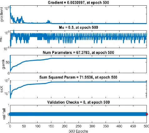
Fig. 4 represents the training state for the neural network
model. As indicated earlier, the number of error iteration is equivalent to 500. The network is processed for 500 epochs, at which 285 epoch attains the best validation.
Figure 5. Evaluation of the testing performance of Bayesian regularization (BR) and Levenberg-Marquardt (LM) using a varying
number of epochs
From Fig. 5, we can clearly state that the Bayesian regularization algorithm performs better than the Levenberg-Marquardt algorithm in terms of error reduction and compilation time. As the error rate across the different epochs from 1 to1000 consistently gives a minimum value for BR compared to LM. Fig. 6 clearly shows that at epoch 500 the minimum error rate is found for the Bayesian Regularization algorithm.
Figure 6. Error graph for Bayesian Regularization algorithm
4.2 Performance Comparison Based on Different NN Algorithms
The performance measures of precision, recall, accuracy and error rate were considered for the evaluation of NN algorithms. The accuracy refers to the degree of closeness of the true value with the measured value. The precision refers to the performance of the algorithm with highly relevant values. The recall refers to the inclination towards providing more relevant results.
259 various neural network algorithms. Comparative tests are
done using different algorithms such as CGF, BFQS, SCG and their performance matrices are discussed hereunder.
Table 2: Bayesian Regularization Confusion Matrix Predict Positiv
e
Negativ e
Actual
Positive 204 64
Negativ
e 36 464
Levenberg-Marquardt (LM) algorithm is mainly used for solving the minimization problems for non-linear least squared values. LM algorithm works with the combination of the Gauss-Newton method along with the gradient descent method. The performance of LM algorithm is superior in terms of MAE, RMSE etc. compared with other algorithms for a multilayer perceptron (MLP) neural network used for the accurate prediction of the post-dialysis blood urea concentration [17]. The proposed algorithm could achieve a predictive accuracy of 0.269% in a 6-11-1 network topology with linear AFs (Activate Functions) in the input layer and log-Sigmoid AFs in the output layer. Models based on Feed-forward neural network for the prediction of Type I diabetes is presented in [18]. The models use LM algorithm for the training process, which gives 82% accuracy upon validation. Prediction of Blood Glucose levels based on the history of the glucose level, meal intake and insulin injections is presented in [19]. The proposed algorithm uses of Artificial Neural Networks, based on LM algorithm. For the Gauss-Newton approach, the error value is reduced based on finding the least quadrant. Whereas, gradient descent they update the parameters of the steepest-descent direction. From table 3, the number of correctly classified data is seen as 611.
Table 3: Levenberg Marquardt Confusion Matrix Predict
Positive Negative
Actual
Positive 150 118
Negativ
e 93 461
A scaled conjugate gradient (SCG) is a feed-forward neural network based on a supervised learning algorithm. The supervisory learning algorithm Scaled Conjugate Gradient (SCG) was introduced by Martin F Moller in 1991 [20]. The algorithm doesn’t contain any of the user dependent parameters. As the algorithm avoids a time-consuming line search per learning iteration, the performance of the algorithm is superior compared with Standard Back propagation algorithm, Conjugate Gradient Algorithm with line search and Broyden– Fletcher–Goldfarb–Shanno (BFGS) algorithm. SCG algorithm is based on a time-consuming methodology for line search. The idea is to combine the model-trust region approach combined with the conjugate gradient. Among the other conjugate algorithm, SCG may require a greater number of iterations, but lesser computational complexity. From table 4, the number of correctly classified data can be found as 590,
using the SCG algorithm.
Table 4: Scaled Conjugate Gradient Confusion Matrix Predict
Positive Negative
Actual
Positive 153 115
Negativ
e 63 437
Conjugate Gradient using Fletcher is used (CGF) is the norm for the squared of the present gradient to the squared of the prior gradient. Compared to the other algorithms, CGF works much faster but this totally depends on the problem being carried out. From table 5 the number of correctly classified data is identifiable as 602.
Table 5: Fletcher Conjugate Gradient Confusion Matrix Predict
Positive Negative
Actual
Positive 147 121
Negativ
e 45 455
Broyden Fletcher Goldfarb Shanno (BFGS) is main adapted using the quasi-newton method. BFGS algorithm mainly focuses on the data with minimum storage, using linear algebra. BFGS method is used on optimization based on unconstrained fields. From table 6, the number of correctly classified data can be found as 602.
Table 6: BFGS Quasi-Newton Confusion Matrix Predict
Positive Negative
Actual
Positive 157 111
Negativ
e 55 445
5 R
ESULT ANDD
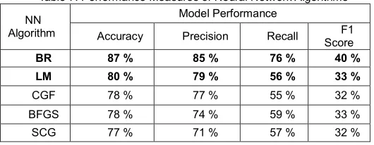
ISCUSSIONThe performance measures (accuracy, precision, recall, and F1 score) were computed for the Type II diabetes dataset, using different NN algorithms.
Table 7: Performance Measures of Neural Network Algorithms
NN Algorithm
Model Performance
Accuracy Precision Recall Score F1
BR 87 % 85 % 76 % 40 %
LM 80 % 79 % 56 % 33 %
CGF 78 % 77 % 55 % 32 %
BFGS 78 % 74 % 59 % 33 %
260 Table 7 demonstrates the accuracy score for BR at 87%, that’s
the accuracy percentage our model is able to predict. Followed by which the precision value that’s 85%, which indicates the accuracy in prediction of True positive values. The recall value here is 76%, where it identifies the actual positive value. The F1 score is 40%, which is the best measure to identify the relation between both precision and recall.
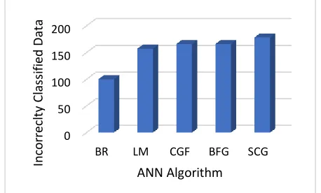
Figure 7. Comparative chart that describes the incorrectly classified data across various NN algorithms
We have analyzed the learning rate and created the network that best fits the problem. Fig. 7 illustrates a comparative study based on incorrect classification of other neural network algorithms has been shown. Compared to other algorithms Bayesian Regularization (BR) sustains the least number of misclassifications.
Table 8: Error Rate of Neural Network Algorithms
BR 36.08
LM 39.15
CGF 45.15
BFGS 55.15
SCG 63.14
The performance in table 8 above indicates that the number of false positives varies between 36.08 to 63.14. SCG algorithm has the largest number of false positives, while the Bayesian Regularization has the smallest number. Accuracy of the system is closely related to the number of learning samples used for the training process.
Figure 8. Comparative chart that describes the correctly classified data across various NN algorithms
Fig. 8 indicates the correctly classified cases for each algorithm. Compared to the other algorithms, Bayesian regularization shows a considerably high number of 668 instances being correctly classified. Classification chart identifies the number of instances that are correctly classified across various algorithms, based on the predicted accuracy. Feedforward neural network approaches have been discussed in this paper, for performance evaluation and error rate. The results of this study validate the premise that Bayesian Regularization attains better performance rate than other neural network algorithms. Cross-validation nature of LM could be reduced or eliminated using BR. It is more robust as well as works with nonlinear problems. Therefore, compared to the other methods BR is found to be an optimal solution both in terms of predictive ability and error reduction.
6 C
ONCLUSIONIn this paper, the Bayesian Neural Network architecture is used for predictive analysis of type II diabetes. With an intention to select the optimal algorithm, a comparative study over the Pima diabetes dataset using various neural network algorithm was performed. Bayesian Regularization showed the best results against the other algorithms, in terms of accuracy and error minimization. The architecture gained up to 87 % accuracy at the error rate of 0.11429, at epoch 285. Different neural network algorithms were tested for comparative study based on the proposed architecture to clearly identify the difference in the error value and computational values. Future works can be carried out by using different deep learning and ANFIS techniques. Then a strong evaluation of various Machine Learning algorithms could be ensembled and various techniques can be compared with respect to its strengthens.
R
EFERENCES[1] E. O. Olaniyi and K. Adnan, ―Onset Diabetes Diagnosis Using Artificial Neural Network,‖ Int. J. Sci. Eng. Res., vol. 5, no. 10, pp. 754–759, 2014.
[2] D. Dutta, D. Paul, and P. Ghosh, ―Analysing Feature Importances for Diabetes Prediction using Machine Learning,‖ 2018 IEEE 9th Annu. Inf. Technol. Electron. Mob. Commun. Conf. IEMCON 2018, pp. 924–928, 2019.
[3] H. Abbas, L. Alic, M. Rios, M. Abdul-Ghani, and K. Qaraqe, ―Predicting diabetes in healthy population through machine learning,‖ Proc. - IEEE Symp. Comput. Med. Syst., vol. 2019-June, pp. 567–570, 2019.
[4] E. Dogantekin, A. Dogantekin, D. Avci, and L. Avci, ―An intelligent diagnosis system for diabetes on Linear Discriminant Analysis and Adaptive Network Based Fuzzy Inference System: LDA-ANFIS,‖ Digit. Signal Process. A Rev. J., vol. 20, no. 4, pp. 1248–1255, 2010.
[5] R. C. Deo, ―Machine learning in medicine,‖ Circulation, vol. 132, no. 20, pp. 1920–1930, 2015.
[6] D. R. Sarvamangala and R. V. Kulkarni, ―Swarm intelligence algorithms for medical image registration: A comparative study”,Proc. of International Conference on Computational Intelligence, Communications, and
0 50 100 150 200
BR LM CGF BFG SCG
In
co
rr
ecl
ty
C
las
si
fi
ed
D
at
a
ANN Algorithm
540 560 580 600 620 640 660 680
BR LM CGF BFG SCG
C
o
rr
ect
ly
C
las
si
fi
ed
D
at
a
261
Business Analytics, vol. 776, pp. 451-465, 2017. [7] S. Larabi-Marie-Sainte, L. Aburahmah, R. Almohaini,
and T. Saba, ―Current techniques for diabetes prediction: Review and case study,‖ Appl. Sci., vol. 9, no. 21, 2019.
[8] Z. Soltani and A. Jafarian, ―A New Artificial Neural Networks Approach for Diagnosing Diabetes Disease Type II,‖ Int. J. Adv. Comput. Sci. Appl., vol. 7, no. 6, pp. 89–94, 2016.
[9] A. Ashok, S. Smitha, and M. H. K. Krishna, ―Attribute reduction based anomaly detection scheme by clustering dependent oversampling PCA,‖ 2016 Int. Conf. Adv. Comput. Commun. Informatics, ICACCI 2016, pp. 1298–1304, 2016.
[10] H. Balaji, N. C. S. . Iyengar, and R. D. Caytiles, ―Optimal Predictive analytics of Pima Diabetics using Deep Learning,‖ Int. J. Database Theory Appl., vol. 10, no. 9, pp. 47–62, 2017.
[11] P. Rahimloo and A. Jafarian, ―Prediction of Diabetes by Using Artificial Neural Network, Logistic Regression Statistical Model and Combination of Them,‖ Bull. la Société R. des Sci. Liège, vol. 85, pp. 1148–1164, 2016.
[12] A. Manghat and A. Ashok, ―Abnormality prediction in high dimensional dataset among semi supervised learning approaches,‖ 2017 Int. Conf. Adv. Comput. Commun. Informatics, ICACCI 2017, vol. 2017-Janua, pp. 1494–1499, 2017.
[13] S. Mortajez and A. Jamshidinezhad, ―An Artificial Neural Network Model to Diagnosis of Type II Diabetes.‖
[14] ―Pima-Indians-Diabetes.‖ [Online]. Available: archive.ics.uci.edu.
[15] E. Sariev and G. Germano, ―Bayesian regularized artificial neural networks for the estimation of the probability of default,‖ Quant. Financ., vol. 20, no. 2, pp. 311–328, 2020.
[16] M. Kayri, ―Predictive abilities of Bayesian regularization and levenberg-marquardt algorithms in artificial neural networks: A comparative empirical study on social data,‖ Math. Comput. Appl., vol. 21, no. 2, 2016 [17] Azar, A. Taher. "Fast neural network learning
algorithms for medical applications." Neural Computing and Applications. vol. 23, no.3-4, pp. 1019-1034, 2013. [18] Zhang, Yinghui, Z. Lin, Y. Kang, R. Ning, and Y. Meng.
"A feed-forward neural network model for the accurate prediction of diabetes mellitus." Int. J. of Scientific and Technology Research, vol. 7, no. 8, pp. 151-155, 2018. [19] Robertson, Gavin, D. Lehmann, W. Sandham, and D. Hamilton. "Blood glucose prediction using artificial neural networks trained with the AIDA diabetes simulator: a proof-of-concept pilot study." Journal of Electrical and Computer Engineering, 2011.
![Table 1: ANALYSIS OF PIMA DIABETES DATASET [14] Attributes Range](https://thumb-us.123doks.com/thumbv2/123dok_us/8635439.1425147/2.612.333.559.337.483/table-analysis-pima-diabetes-dataset-attributes-range.webp)