promoting access to White Rose research papers
White Rose Research Online
[email protected]
Universities of Leeds, Sheffield and York
http://eprints.whiterose.ac.uk/
This is an author produced version of a paper published in
Neural Computing
and Applications
.
White Rose Research Online URL for this paper:
Published paper
Camastra, F., Filippone, M. (2009)
A comparative evaluation of nonlinear
dynamics methods for time series prediction
, Neural Computing and Applications,
18 (8), pp. 1021-1029
A comparative evaluation of Nonlinear Dynamics
Methods for Time Series Prediction
Francesco Camastra
Department of Applied Science, University of Naples Parthenope Centro Direzionale Isola C4 - 80133 Napoli, Italy
e-mail: [email protected]
Maurizio Filippone
Department of Computer Science, University of Sheffield
Regent Court, 211 Portobello Street, Sheffield, S1 4DP, United Kingdom e-mail: [email protected]
Abstract
A key problem in time series prediction using autoregressive models is to fix the model order, namely the number of past samples required to model the time series adequately. The estimation of the model order using cross-validation may be a long process. In this paper, we inves-tigate alternative methods to cross-validation, based on nonlinear dy-namics methods, namely Grassberger-Procaccia, K´egl, Levina-Bickel and False Nearest Neighbors algorithms. The experiments have been performed in two different ways. In the first case, the model order has been used to carry out the prediction, performed by a SVM for regres-sion on three real data time series showing that nonlinear dynamics methods have performances very close to the cross-validation ones. In the second case, we test the accuracy of nonlinear dynamics methods in predicting the known model order of synthetic time series. In this case most of the methods have yielded a correct estimate and when the estimate was not correct, the value was very close to the real one.
1
Introduction
in time series prediction is to fix themodel order, namely the number of past samples required to model the time series adequately. In principle, cross-validation[6, 26] is the simplest solution, just picking the model order which gives the lowest prediction error. The computational cost of cross-validation, however, may be high; an estimate of the model order can be helpful, either to be used directly, or to narrow down the range for cross-validation. The problem of estimating the order of a model is crucial not only in time series analysis, but in data modeling in general. Popular approaches to model order estimation are based on concepts of Information Theory and Statis-tics, such as the Akaike Information Criterion (AIC) [2], methods based on the Minimum Description Length (MDL) principle [21], Bayesian Informa-tion Criterion (BIC) [23], and hypothesis testing [3, 16]. Although these methods have a solid theoretical foundation, the model assumption plays a key role, and a deviation from the real model can lead to a degradation of their performances [9]. A robust approach to the model order estimation in the framework of uncertain statistics can be found in [9]. In this paper, we focus on the time series prediction problem. In this context, the False Nearest Neighbors algorithms has already been used in several time series prediction applications [4] to estimate the model order. Here, we compare a set of methods for model order estimation based on nonlinear dynamics the-ory, namely Grassberger-Procaccia, K´egl, Levina-Bickel, and False Nearest Neighbors algorithms. The model order is used to carry out the prediction by means of a Support Vector Machine for Regression (SVM) [20, 22, 30]. We assess the performances of the estimators on the basis of the prediction accuracy achieved by the SVMs trained using the selected model order. We also investigate the effectiveness of nonlinear dynamics methods comparing their performances with those obtained by cross-validation. Finally, we test the accuracy of nonlinear dynamics methods in predicting the known model order of synthetic time series. The paper’s structure is as follows: in Section 2 a description of the nonlinear dynamics methods investigated is provided; in Section 3 some experimental results are reported; in Section 4 conclusions are drawn.
2
Nonlinear Dynamics Methods
the model order (d−1). Nonlinear Dynamics methods can be used for the
model reconstruction of the time series. This is performed by the method of delays [7, 19]. The time series can be represented as a series of a set of points
{X~(t) :X~(t) = [x(t), x(t−1), . . . , x(t−d+ 1)]}in ad-dimensional space. If
dis adequately large, between the manifold1 M obtained by the pointsX~(t)
and the attractorU of the dynamic system that generated the time series, there is a diffeomorphism2. TheTakens-Ma˜n´e embedding theorem3 [15, 27] states that to obtain a faithful reconstruction of the system dynamics, it must be
2S+ 1≤d (1)
whereS is the dimension of the system attractor U and dis called the em-bedding dimensionof the system. Hence it is adequate to measureSto infer the embedding dimensiondand the model orderd−1. A unique definition of the dimension has not been given yet. Popular definitions of set dimensions are the Box-Counting Dimension [18] and the Correlation dimension [8]. In the next sections, we shall discuss three methods to estimate attractor dimension (Grassberger-Procaccia, Levina-Bickel and K´egl methods) and a method to estimate the embedding dimension, without using Takens-Ma˜n´e embedding theorem (False Nearest Neighbors method).
2.1 K´egl’s algorithm
Let Ω ={~x1, ~x2, . . . , ~xℓ} be a set of points inRn of cardinality ℓ. The Box-Counting dimension (orKolmogorov capacity)DB of the set Ω is defined as follows [18]: if ν(r) is the number of the boxes (i.e. hypercubes) of size r
needed to cover Ω, then DB is
DB = lim r→0
ln(ν(r))
ln(1r) (2)
1A manifold [34] is a mathematical space in which every point has a neighborhood which
resembles Euclidean space, but in which the global structure may be more complicated. In a one-dimensional manifold (e.g. a line, a circle) every point has a neighborhood that looks like a segment of a line. In a two-dimensional manifold (e.g. a plane, the surface of a sphere) the neighborhood looks like a disk. Rnis a n-dimensional manifold.
2M is
diffeomorphic to U iff there is a differentiable map m:M 7→U whose inverse
m−1exists and is also differentiable.
3Takens-Ma˜n´e embedding theorem is a consequence of a
Whitney Embedding The-orem [32] stating that a generic map from an S-dimensional manifold to a (2S +
1)-dimensional Euclidean space is anembedding, i.e. the image of the S-dimensional mani-fold is completely unmani-folded in the larger space. Therefore two points in theS-dimensional
Recently K´egl [14], has proposed a fast algorithm (K´egl’s algorithm) to esti-mate the Box-Counting dimension. The algorithm was originally proposed for intrinsic data dimensionality estimation. In this paper, we propose a novel application of K´egl’s algorithm, consisting in the dimension estima-tion of an attractor. K´egl’s algorithm is based on the observaestima-tion that
ν(r) is equivalent to the cardinality of the maximum independent vertex set M I(Gr) of the graph Gr(V, E) with vertex set V = Ω and edge set
E ={(~xi, ~xj)|d(~xi, ~xj) < r}. K´egl has proposed to estimate M I(G) using the following greedy approximation. Given a data set Ω, we start with an empty set C. In an iteration over Ω, we add to C data points that are at distance of at leastr from all elements of C. The cardinality of C, after ev-ery point in Ω has been visited, is the estimate ofν(r). The Box-Counting dimension estimate is given by:
DB =−
lnν(r2)−lnν(r1) lnr2−lnr1
(3)
wherer2 and r1 are values that can be set up heuristically.
It can be proven [14] that the complexity of Kegl’s algorithm is given by
O(DBℓ2), whereℓandDB are the cardinality and the dimensionality of the data set, respectively.
2.2 Grassberger-Procaccia algorithm
TheCorrelation dimension [8] of a set Ω is defined as follows. If the corre-lation integral Cm(r) is defined as:
Cm(r) = lim ℓ→∞
2
ℓ(ℓ−1) ℓ
X
i=1
ℓ
X
j=i+1
I(k~xj−~xik ≤r) (4)
whereI is anindicator function4, then the Correlation dimensionDof Ω is:
D= lim r→0
ln(Cm(r))
ln(r) (5)
It can be proved that the Correlation Dimension is a lower bound of the Box-Counting Dimension. The most popular method to estimate Corre-lation dimension is the Grassberger-Procaccia algorithm [8]. This method consists in plotting ln(Cm(r)) versus ln(r). The Correlation dimension is the slope of the linear part of the curve (see Figure 1a). For increasing values
4I
of d one can notice a saturation effect. The limit value is the correlation dimension.
The computational complexity of the Grassberger-Procaccia algorithm is
O(ℓ2s) whereℓis the cardinality of the data set andsis the number of differ-ent times that the integral correlation is evaluated, respectively. This imple-mentation was adopted for the experiments reported in Section 3. However, there are efficient implementations of the Grassberger-Procaccia algorithm whose complexity does not depend on s. For these implementations, the computational complexity is O(ℓ2).
2.3 Levina-Bickel Algorithm
The Levina-Bickel algorithm provides a maximum likelihood estimate of the correlation dimension. Like the K´egl’s algorithm, the Levina-Bickel algo-rithm was proposed for the estimation of the intrinsic data dimensionality. Therefore the application of the Levina-Bickel algorithm for estimating the dimension of an attractor is a novelty. The Levina-Bickel algorithm derives the maximum likelihood estimator (MLE) of the intrinsic dimensionalityD
of a manifold Ω = (~x1, . . . , ~xℓ). The dataset Ω represents an embedding of a lower-dimensional sample, i.e. ~xi =g(Yi) where Yi are sampled from an unknown smooth density f on RD with D < n, g is a smooth mapping. This last assumption guarantees that close datapoints inRD are mapped to close neighbors in the embedding.
That being said, we fix a data point ~x ∈ Rn assuming that f(~x) is con-stant in a sphere S~x(r) centered in ~x of radius r and we view Ω as a homogeneous Poisson process in S~x(r). Given the inhomogeneous process
{P(t, ~x),0≤t≤r}
P(t, ~x) = ℓ
X
i=1
I(~xi∈S~x(t)), (6)
which counts the datapoints whose distance from ~x is less than t. If we approximate it by means a Poisson process and we neglect the dependence on~x, the rate λ(t) of the process P(t) is given by:
λ(t) =f(~x)V(D)DtD−1
, (7)
whereV(D) is the volume of aD-dimensional unit hypersphere.
θ=logf(~x), the log-likelihood of the processP(t) [25] is:
L(D, θ) =
Z r
0
logλ(t)dP(t)−
Z r
0
λ(t)dt. (8)
The equation describes an exponential family for which a maximum like-lihood estimator exists with probability that tends to 1 as the number of samples ℓ tends to infinity. The maximum likelihood estimator is unique and must satisfy the following equations:
∂L ∂θ =
Z r
0
dP(t)−
Z r
0
λ(t)dt=P(r)−eθV(D)rD = 0. (9)
∂L ∂D = 1 D + V′
(D)
V(D)
P(r) +
Z r
0
log t dP(t) +
−eθV(D)rD
log r+V
′
(D)
V(D)
= 0. (10)
If we plug the equation (9) into the equation (10) we obtain the maximum likelihood estimate for the dimensionalityD:
ˆ
Dr(~x) =
1
P(r, ~x) P(r,~x)
X
j=1
log r Tj(~x)
−1
, (11)
whereTj(~x) denotes the Euclidean distance between ~x and its j-th nearest neighbor.
Levina and Bickel suggest to fix the number of the neighborsk rather than the radius of the spherer. Therefore the estimate becomes:
ˆ
Dk(~x) =
1
k−1 k−1 X
j=1
logTk(~x) Tj(~x)
−1
. (12)
The estimate of the dimensionality is obtained averaging on all points of the data set Ω, that is :
ˆ
Dk= 1 ℓ ℓ X i=1 ˆ
Dk(~xi) (13)
The estimate of the dimensionality depends on the value of k. Levina and Bickel suggest to average over a range of values of k=k1, . . . , k2 obtaining the final estimate of the dimensionality, i.e.
ˆ
D= 1
k2−k1+ 1 k=k2
X
k=k1 ˆ
Regarding the computational complexity, the Levina-Bickel algorithm re-quires a sorting algorithm5, whose complexity isO(ℓlogℓ), where ℓdenotes
the cardinality of the data set. Hence the computational complexity for es-timating ˆDk is O(kℓ2logℓ), where k denotes the numbers of the neighbors that have to be considered. Besides, Levina and Bickel suggest to consider an average estimate repeating the estimate Dk s times, where s is the dif-ference between the maximum and the minimum value that k can assume, i.e. k2 and k1, respectively. Therefore the overall computational complexity
of the Levina-Bickel algorithm isO(sℓ2logℓ).
The Levina-Bickel algorithm provides an optimal estimate of the correlation dimension. This topic has been widely investigated in nonlinear dynamics, e.g. [24, 28]. In particular, Takens proposed an algorithm that provides a maximum likelihood estimate, like the Levina-Bickel algorithm. The dif-ference between the Takens and Levina-Bickel algorithms is the following. The former provides an estimate that depends on a radiusr that has to be fixed properly; the latter depends on the number, chosen appropriately, of the neighbors that have to be taken into account for each datapoint of the manifold.
2.4 Method of False Nearest Neighbors
The K´egl, Grassberger-Procaccia and Levina-Bickel algorithms estimate the attractor dimension and compute the model order of the time series by the Takens-Ma˜n´e embedding theorem. An alternative approach is proposed by theFalse Nearest Neighbors method [4, 13]. This method estimates directly the embedding dimension without using the Takens-Ma˜n´e theorem. The False Nearest Neighbors method is based on a simple geometric concept. If the dimensiondused to reconstruct the attractor is too small, many points that appearnear will become widely separated whend+ 1 dimensions are used in the attractor reconstruction. Nearest neighbor points that show this wide separation when comparing their distance in dimension d and d+ 1 are calledFalse Nearest Neighbors in dimensiond. Conversely, true nearest neighbors will remain near each other in attractor reconstructions of bothd
and d+ 1 dimensions. More formally a pair of points are considered False Nearest Neighbors in dimension d if R
2
d+1(j) R2
d(j)
> α where Rd(j) andRd+1(j)
are respectively the Euclidean distance between thejth point and its nearest neighbors indandd+ 1 dimensions andα is an heuristic threshold. Typical
5The complexity of effective sorting algorithms (e.g. mergesort and heapsort) isℓlogℓ,
values for α are suggested in [4]. The adequacy of dimension d for recon-structing an attractor can be evaluated by calculating for each data point of the attractor the nearest neighbors in dimension d and then evaluating the percentage of False Nearest Neighbors. Then the percentage of False Nearest Neighbors is plotted versus the dimensiond. The lowest dimension corresponding to this minimum value of the percentage of False Nearest Neighbors is the embedding dimension. The main operation involved in the method is the nearest neighbor search. The time complexity of finding the nearest neighbor of a point in addimensional set of cardinalityℓ, isO(dℓ). Since we are interested in computing the the nearest neighbors for all the
ℓ points of the set, we can simply use the nearest neighbor algorithm for all the ℓ points, that is O(dℓ2) in total. It is worth noting, however, that the complexity of this approach can be reduced6 by storing the data in suit-able data structures [31]. Once we obtain the nearest neighbors for the ℓ
data points, we need to compute the distances in the augmented space and compute the percentage of false nearest neighbors; these operations have a complexity that is lower than O(dℓ2). Finally, the procedure has to be repeated for all the values ofdfor which we are interested in computing the percentage of False Nearest Neighbors (FNN).
It is necessary to remark that in literature [4] when the FNN method is applied, the obtained result is used directly as the model order estimate. In the rest of the manuscript this procedure is used.
3
Experimental Results
The False Nearest Neighbors, Grassberger-Procaccia, K´egl and Levina-Bickel algorithms have been tested on three synthetic time series and on three benchmarks of real data.
3.1 Real Data Time Series
The False Nearest Neighbors, Grassberger-Procaccia, K´egl and Levina-Bickel algorithms have been tested on three real data time series, e.g. the Data Set A [10] of the Santa Fe time series competition, the Paris-14E Parc Montsouris [33] and theDSVC1 [1] time series7. On the real data sets, we
have compared the prediction accuracy obtained by cross-validation with
6In our implementation, we use the linear search having complexityO(dℓ2). 7
Paris-14E Parc Montsouris and DSVC1 time series can be downloaded from www.knmi.nl/samenw/eca and www.cpdee.ufmg.br/∼MACSIN/services/data/data.htm,
the SVM for regression trained using the model order estimated by the pre-sented methods. In these experiments, we have used 10-fold cross-validation. We recall that inK-fold cross-validation, the training set is partitioned into
K subsets. Of the K subsets, a single subset is retained as the validation data for testing the model, and the remaining K −1 subsets are used as training data. The cross-validation process is then repeated K times, i,e. the folds, with each of the K subsets used exactly once as the validation data. TheK results from the folds then can be averaged to produce a single estimation.
3.1.1 Data Set A
Data Set A is a real data time series, formed by 1000 samples, generated by a Lorenz-like chaotic system, implemented by NH3-FIR lasers. Firstly the
-4 -3 -2 -1 0 ln r
-12 -10 -8 -6 -4 -2 0
ln C
1 2 3 4 5
d 0
0.2 0.4 0.6 0.8
[image:11.595.134.487.171.331.2]rate
Figure 1: The Grassberger-Procaccia (a) and False Nearest Neighbors (b) algorithms on Data Set A.
0 50 100 150 200 250 300
0 25 50 75 100 125 150 175
0 50 100 150 200 250 300
0 25 50 75 100 125 150 175
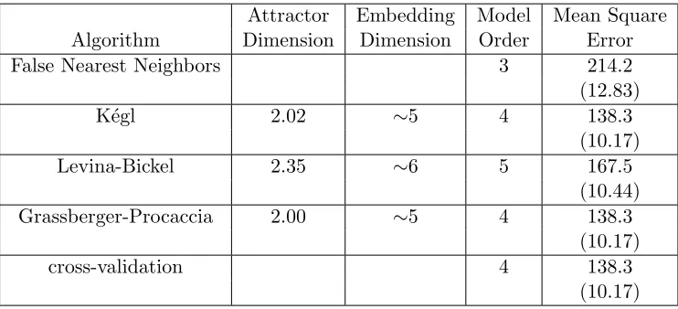
[image:11.595.132.486.470.579.2]Attractor Embedding Model Mean Square
Algorithm Dimension Dimension Order Error
False Nearest Neighbors 3 214.2
(12.83)
K´egl 2.02 ∼5 4 138.3
(10.17)
Levina-Bickel 2.35 ∼6 5 167.5
(10.44)
Grassberger-Procaccia 2.00 ∼5 4 138.3
(10.17)
cross-validation 4 138.3
[image:12.595.126.497.129.298.2](10.17)
Table 1: The False Nearest Neighbors, K´egl, Grassberger-Procaccia and cross-validation method on Data Set A. Average error is reported in brackets.
3.1.2 Paris-14E Parc Montsouris
Paris-14E Parc Montsouris is a real data time series formed by the daily average temperatures, expressed in tenths of Celsius degrees, in Paris. The time series covers the whole period from January 1 1958 to December 31 2001 and has 15706 samples. The former 64% of time series (10043 samples) has been used for the training set, while the latter one has been used for the test set, formed by 5663 samples. We have estimated the model order using the False Nearest Neighbors, Grassberger-Procaccia, K´egl and Levina-Bickel algorithms and we have performed the prediction stage using SVM-Light. Even in this case, we have used the gaussian kernel, setting the variance using cross-validation. As a comparison we have also estimated the model order by means of the cross-validation. The results on the test set, expressed in terms of quadratic loss, are reported in the table 2 and shown in figure 3.
3.1.3 DSVC1
Attractor Embedding Model Mean
Algorithm Dimension Dimension Order Square Error
False Nearest Neighbors 5 436.5
(16.66)
K´egl 4.03 ∼9 8 434.3
(16.65)
Levina-Bickel 5.96 ∼13 12 434.6
(16.65)
Grassberger-Procaccia 4.91 ∼11 10 429.6
(16.53)
cross-validation 10 429.6
[image:13.595.126.496.129.298.2](16.53)
Table 2: The False Nearest Neighbors, K´egl, Grassberger-Procaccia and cross-validation method on the Data Set Paris-14E Parc Montsouris. Aver-age error is reported in brackets.
and Levina-Bickel algorithms. The prediction stage was performed using SVM-Light. Even in this case, we have used the gaussian kernel, setting the variance using cross-validation. The estimates of the attractor dimen-sion using Grassberger-Procaccia, K´egl and Levina-Bickel algorithms are respectively 2.20, 2.14 and 2.26. Since the attractor dimension of data set A is∼2.26, the estimates of the algorithms can be considered satisfactory. As a comparison the model order was also estimated by means of cross-validation. The results expressed on the test set are reported in the table 3
0 100 200 300 400 500
-50 0 50 100 150 200 250
0 100 200 300 400 500
0 50 100 150 200 250
[image:13.595.137.486.502.611.2]and are shown in figure 4. Finally, the average CPU times required by all
Attractor Embedding Model Mean
Algorithm Dimension Dimension Order Square Error
False Nearest Neighbors 6 0.10
(0.23) K´egl 2.14 [5. . .6] [4. . .5] [0.10. . .0.075]
([0.26. . .0.20])
Levina-Bickel 2.26 ∼6 5 0.075
(0.20) Grassberger-Procaccia 2.20 [5. . .6] [4. . .5] [0.10. . .0.075]
([0.26. . .0.20])
cross-validation 5 0.075
[image:14.595.125.510.154.323.2](0.20)
Table 3: The False Nearest Neighbors, K´egl, Grassberger-Procaccia and cross-validation method on DSVC1 Time Series. Average error is reported in brackets. Since the model order estimated by Grassberger-Procaccia and Kegl is between 4 and 5, mean square error is between 0.10 and 0.075, and average error is between 0.26 and 0.20.
nonlinear methods for estimating the model order are reported in table 4. Note that in the FNN method, percentage of false neighbors has been com-puted up to a maximum dimension of 12. The experiments were performed on a Windows Vista8 PC with a Dual Core 1,83 GhZ Intel Processor and 3 GByte RAM. False Nearest Neighbors, Grassberger-Procaccia and cross-validation were implemented in C/C++, whereas K´egl and Levina-Bickel were implemented using Mathematica9.
8
Windows Vista is a registered trademark of Microsoft Inc.
9
0 100 200 300 400 500 -3
-2 -1 0 1 2 3
0 100 200 300 400 500
[image:15.595.134.487.127.240.2]-3 -2 -1 0 1 2
Figure 4: Chua Time Series. The original target data and the results yielded by SVM (model order = 5) are shown on the left and the right respectively.
Data Set A Paris-14E DSVC1
Algorithm Parc Montsouris
False Nearest Neighbors 1 65 5
K´egl 32 1230 202
Levina-Bickel 30 1170 189
Grassberger-Procaccia 16 536 106
cross-validation 125 2810 756
Table 4: Average CPU Time, measured in seconds, required by False Nearest Neighbors, K´egl, Grassberger-Procaccia and cross-validation methods for estimating the model order on Data Seta A, Paris-14E Parc Montsouris and DSVC1 benchmarks.
3.2 Synthetic Time Series
The synthetic time series10 have been generated with a fixed and known model order, and we were interested in evaluating the ability of the presented methods to estimate it. We generated three time series in the following way:
x(t+ 1) = d
X
i=1
a(i)x(t−i+ 1) +a(0) +ε
The vector~acontains the coefficients of the linear combination of the past
d samples, and ε ∼ N(0, σ) is a white Gaussian noise term. The time se-ries have been generated using the parameters shown in table 5. The sese-ries have been generated starting from few random numbers between −1 and
10
[image:15.595.137.473.295.397.2]a(0) σ ~a
d= 4 -0.2 0.005 (-0.38, 0.493, 0.485, -0.535)
d= 5 -0.05 0.005 (-0.5, 0.3, 0.4, 0.25, -0.35)
[image:16.595.160.453.126.187.2]d= 6 -0.3 0.005 (0.22, 0.38, -0.26, -0.23, -0.126, 0.4)
Table 5: Parameters of the three synthetic data sets.
1 (that have been discarded), and have length 10000. Tables 6, 7 and
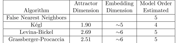
Attractor Embedding Model Order
Algorithm Dimension Dimension Estimated
False Nearest Neighbors 4
K´egl 1.66 ∼4 3
Levina-Bickel 1.95 ∼5 4
[image:16.595.135.473.418.501.2]Grassberger-Procaccia 1.98 ∼5 4
Table 6: The False Nearest Neighbors, K´egl, Grassberger-Procaccia methods on a Synthetic Data series, whose model order is 4.
Attractor Embedding Model Order
Algorithm Dimension Dimension Estimated
False Nearest Neighbors 5
K´egl 1.90 ∼5 4
Levina-Bickel 2.69 ∼6 5
Grassberger-Procaccia 2.51 ∼6 5
Table 7: The False Nearest Neighbors, K´egl, Grassberger-Procaccia methods on a synthetic time series, with model order 5.
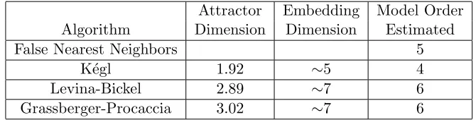
Attractor Embedding Model Order
Algorithm Dimension Dimension Estimated
False Nearest Neighbors 5
K´egl 1.92 ∼5 4
Levina-Bickel 2.89 ∼7 6
[image:17.595.137.472.129.214.2]Grassberger-Procaccia 3.02 ∼7 6
Table 8: The False Nearest Neighbors, K´egl, Grassberger-Procaccia methods on a synthetic time series, with model order 6.
in all time series.
4
Conclusion
In this paper, we have investigated four nonlinear dynamics methods, i.e. False Nearest Neighbors, Grassberger-Procaccia, K´egl and Levina-Bickel al-gorithms, to estimate the model order of a time series, namely the number of past samples required to model the time series adequately. The experiments have been performed in two different ways. In the first case, the model order has been used to carry out the prediction, performed by a SVM for regression on three real data time series. The experiments have shown that the model order estimated by nonlinear dynamics methods is quite close to the one estimated using cross-validation. In the second case the experiments have been performed on synthetic time series, generated with a fixed and known model order, and we were interested in evaluating the ability of the presented methods to estimate it. In this case most of the methods have yielded a correct estimate and when the estimate was not correct, the value was very close to the real one.
References
[1] L.A. Aguirre, G.G. Rodrigues, E.M. Mendes, “Nonlinear identification and cluster analysis of chaotic attractors from a real implementation of Chua’s circuit”, International Journal of Bifurcation and Chaos 6(7), 1411-1423, 1997.
[2] H. Akaike, “A new look at the statistical model identification,” IEEE Transactions on Automatic Control, vol.19, no.6, pp. 716-723, Dec 1974
[3] T. W. Anderson, (1963). “Determination of the order of dependence in normally distributed time series”, in Time series Analysis (M. Rosen-blatt, Ed.), John Wiley & Sons, 1963, pp. 425-446.
[4] H.D.I. Arbabanel,Analysis of Observed Chaotic Data, Springer-Verlag, 1996.
[5] L.O. Chua, M. Komuro, T. Matsumoto, “The double scroll”, IEEE Transactions on Circuits and Systems, 32(8), 797-818, 1985.
[6] R.O. Duda, P.E. Hart and D.G. Stork, Pattern Classification, Wiley Classification, John Wiley and Sons, New York, 2000.
[7] J.P. Eckmann and D. Ruelle, “Ergodic Theory of Chaos and Strange Attractors”,Review of Modern Physics, 57, 617-659, 1985.
[8] P. Grassberger and I. Procaccia, “Measuring the Strangeness of Strange Attractors”,Physica, D9, 189-208, 1983.
[9] D. Hirshberg and N. Merhav, “Robust methods for model order es-timation”. IEEE Transactions on Signal Processing 44, pp. 620-628, 1996.
[10] U. H¨ubner, C.O. Weiss, N.B. Abraham and D. Tang, “Lorenz-Like Chaos in NH3-FIR Lasers”, Time Series Prediction. Forecasting the
Future and Understanding the Past, 73-104, Addison Wesley, 1994.
[11] T. Joachim, “Making large-Scale SVM Learning Practical”, Advances in Kernel Methods - Support Vector Learning, MIT Press, 1999.
[13] M.B. Kennel, R. Brown and H.D.I. Arbabanel, “Determining Embed-ding Dimension for Phase-Space Reconstruction using a Geometrical Construction”, Physical Review A, 45(6), 3403-3411, 1992.
[14] B. K´egl, “Intrinsic Dimension Estimation Using Packing Numbers”,
Advances in Neural Information Processing 15, MIT Press, 2003.
[15] R. Ma˜n´e, “On the dimension of compact invariant sets of certain nonlin-ear maps”,Dynamical Systems and Turbolence, Warwick 1980, Lecture Notes in Mathematics no. 898, 230-242, Springer-Verlag, 1981.
[16] N. Merhav, “The estimation of the model order in exponential families”.
IEEE Transactions on Information Theory 35(5): 1109-1114, 1989.
[17] K-R. M¨uller, G. R¨atsch, J. Kohlmorgen, A. Smola, B. Sch¨olkopf, V. Vapnik, “Time Series Prediction using support vector regression and neural network”, in T. Higuchi and Y. Takizawa (eds.) Proceedings of Second International Symposium on Frontiers of Time Series Mod-elling: Nonparametric Approach to Knowledge Discovery, Institute of mathematical statistic publication, 2000.
[18] E. Ott, Chaos in Dynamical Systems, Cambridge University Press, 1993.
[19] N. Packard, J. Crutchfield, J. Farmer and R. Shaw, “Geometry from a time series”, Physical Review Letters, 45(1), 712-716, 1980.
[20] B. Sch¨olkopf and A. Smola,Learning with Kernels, MIT Press, 2002.
[21] J. Rissanen, ”Modeling by shortest data description,” Automatica , vol. 14, no. 5, pp. 465-471, 1978.
[22] J. Shawe-Taylor, N. Cristianini, Kernel Methods for Pattern Analysis, Cambridge University Press, 2004.
[23] G. Schwarz, ”Estimating the dimension of a model,” Annals of Statis-tics, vol. 6, no. 2, pp. 461-464, 1978.
[24] R. L. Smith, Optimal Estimation of Fractal Dimension. Nonlinear Mod-eling and Forecasting, M. Casdagli, S. Eubank (eds.). SFI Studies in the Sciences of Complexity vol. XII, Addison-Wesley, New York, 1992, 115-135.
[26] M. Stone, “Cross-validatory choice and assessment of statistical predic-tion”, Journal of the Royal Statistical Society, 36(1), 111-147, 1974.
[27] F. Takens, “Detecting strange attractor in turbolence”,Dynamical Sys-tems and Turbolence, Warwick 1980, Lecture Notes in Mathematics no. 898, 366-381, Springer-Verlag, 1981.
[28] F. Takens, On the Numerical Determination of the Dimension of an At-tractor. Dynamical Systems and Bifurcations, Proceedings Groningen 1984, B. Braaksma, H. Broer and F. Takens (eds.), Lecture Notes in Mathematics No. 1125, Springer-Verlag, Berlin, 1985, 99-106.
[29] H. Tong, Nonlinear Time Series, Oxford University Press, 1990.
[30] V.N. Vapnik.Statistical Learning Theory, John Wiley and Sons, New York, 1998.
[31] P. M. Vaidya, “An O(n log n) Algorithm for the All-Nearest-Neighbors Problem”, Discrete and Computational Geometry 4(1): 101-115, 1989.
[32] H. Whitney, “Differentiable manifolds”, Annals of Mathematics 37, 645-680, 1936.
[33] J.B. Wijngaard , A.M.G. Klein Tank and G.P. Konnen, “Homogeneity of 20th century European daily temperature and precipitation series”, International Journal of Climatology, 23, 679-692, 2003.