This is a repository copy of
Forced oscillations of coronal loops driven by external EIT
waves
.
White Rose Research Online URL for this paper:
http://eprints.whiterose.ac.uk/10487/
Article:
Ballai, I., Douglas, M. and Marcu, A. (2008) Forced oscillations of coronal loops driven by
external EIT waves. Astronomy & Astrophysics, 488 (3). pp. 1125-1132. ISSN 0004-6361
https://doi.org/10.1051/0004-6361:200809833
[email protected] https://eprints.whiterose.ac.uk/ Reuse
Unless indicated otherwise, fulltext items are protected by copyright with all rights reserved. The copyright exception in section 29 of the Copyright, Designs and Patents Act 1988 allows the making of a single copy solely for the purpose of non-commercial research or private study within the limits of fair dealing. The publisher or other rights-holder may allow further reproduction and re-use of this version - refer to the White Rose Research Online record for this item. Where records identify the publisher as the copyright holder, users can verify any specific terms of use on the publisher’s website.
Takedown
If you consider content in White Rose Research Online to be in breach of UK law, please notify us by
DOI:10.1051/0004-6361:200809833
c
ESO 2008
&
Astrophysics
Forced oscillations of coronal loops driven by EIT waves
⋆
I. Ballai
1, M. Douglas
1, and A. Marcu
21 Solar Physics and Space Plasma Research Centre (SP2RC), Dept. of Applied Mathematics, University of Sheffield, Hicks Building,
Hounsfield Road, Sheffield, S3 7RH, UK e-mail:[email protected]
2 Babes-Bolyai University, Dept. of Theoretical and Computational Physics, 1 Kogalniceanu, 400084 Cluj-Napoca, Romania
Received 24 March 2008/Accepted 9 July 2008
ABSTRACT
Aims.We study the generation of transversal oscillations in coronal loops represented as a straight thin flux tube under the effect of an external driver modelling the global coronal EIT wave. We investigate how the generated oscillations depend on the nature of the driver, and the type of interaction between the two systems.
Methods.We consider the oscillations of a magnetic straight cylinder with fixed-ends under the influence of an external driver modelling the force due to the global EIT wave. Given the uncertainties related to the nature of EIT waves, we first approximate the driver by an oscillatory force in time and later by a shock with a finite width.
Results.Results show that for a harmonic driver the dominant period in the generated oscillation belongs to the driver. Depending on the period of driver, compared to the natural periods of the loop, a mixture of standing modes harmonics can be initiated. In the case of a non-harmonic driver (modelling a shock wave), the generated oscillations in the loop are the natural periods only. The amplitude of oscillations is determined by the position of the driver along the tube. The full diagnosis of generated oscillations is achieved using simple numerical methods.
Key words.magnetohydrodynamics (MHD) – Sun: corona – waves
1. Introduction
Latest high-resolution coronal observations have shown that coronal structures are very dynamic entities with flows and waves propagating along them. Waves and oscillations in coro-nal loops have received increased attention in the last few years due to the possibility to use the observed properties to diagnose not only the magnetic field in these structures, but also the sub-resolution space distribution of loops, plasma properties, etc. (e.g. Roberts et al.1984; Aschwanden et al.1999; Nakariakov et al. 1999; Banerjee et al. 2007; Verth et al. 2007; Arregui et al.2008; Verth & Erélyi2008). One specific type of oscil-lations observed in coronal loops is the fast kink mode which disturbs the symmetry axis of the loop (for a full description of these waves see, e.g. Edwin & Roberts1983) and it is nearly incompressible.
Many of kink waves and oscillations have their origin in the interaction of coronal loops with various external sources and drivers (see, e.g. Hindman & Jain 2008; Erdélyi & Hargreaves2008). One of the possible explanations of oscilla-tions in coronal loops and/or prominence fibrils is that they have their origin in the interaction of these loops with global coronal waves, e.g. EIT waves. EIT waves (Thompson et al.1999) are waves generated by sudden energy releases (flares, coronal mass ejections, etc.) and they are able to propagate over very large distances in the solar low corona.
Observational evidence for large-scale coronal impulses ini-tiated during the early stage of a flare and/or CME has been provided by the EIT instrument onboard SOHO, TRACE/EUV,
⋆ EIT: Extreme-Ultraviolet Imaging Telescope.
STEREO/EUVI. EIT waves propagate in the quiet Sun with speeds of 250–400 km s−1 at an almost constant altitude. At a later stage in their propagation EIT waves can be considered as a freely propagating wavefront which is observed to interact with coronal loops (see, e.g. Wills-Davey & Thompson1999). Using TRACE/EUV 195 Å observations, Ballai et al. (2005) have shown that EIT waves – seen in this wavelength – are waves with average periods of the order of 400 s. Since at the height where the EUV lines are formed, the magnetic field can be considered vertical, EIT waves were interpreted as fast mag-netohydrodynamic (MHD) waves. This interpretation was con-firmed using multi-wavelength STEREO/EUVI observations by Long et al. (2008). Recently, Attrill et al. (2007a,b) proposed that the diffuse EIT coronal bright fronts are due to driven magnetic reconnections between the skirt of the expanding CME mag-netic field and the favorably orientated quiet Sun magmag-netic field. According to this latter model, the propagation process of the front consists of a sequence of successive reconnection events.
Although a large consensus was reached on the trigger mech-anism of these global coronal waves and effects EIT waves can generate, the nature of these large scale disturbances is still un-known, despite the multitudes of models. The main reason of this uncertainty is the lack of high temporal and spatial resolution as well as the limited field of view (in the case of TRACE/EUV).
The present paper investigates the temporal and spatial vari-ations of transversal oscillvari-ations in a coronal loop under the in-fluence of an external driver representing the coronal global EIT waves. Strictly speaking a coronal loop application would re-quire the consideration of an external magnetic field. However, we consider this study as a starting point in a much more
1126 I. Ballai et al.: Forced oscillations of coronal loops driven by EIT waves
t
g
F
EITx
z
y
B
l
Photosphere
[image:3.595.60.286.71.270.2]Photosphere
Fig. 1.A schematic representation of the working model. The straight flux tube, arbitrarily inclined with respect to the vertical direction, is under the influence of different forces which will generate transversal oscillations in the coronal loop which has fixed ends in the dense pho-tosphere.
complex analysis. Due to the uncertainties in resolving the na-ture of EIT waves, we will discuss separately the cases of a harmonic driver and a driver of a finite width with a pulse-like temporal distribution. It should be noted here that the study of the present papers apply not only to EIT waves as external driver, but it could be applied to any external source.
In the next section we introduce the working model and de-rive the governing equation of transversal oscillations based on the principle of force equilibrium in conjunction with the con-tinuity of mass and magnetic flux. The governing equation is solved for the a driving force when its particular form is not specified. Section 3 is devoted to the study of the periodical mo-tion of the coronal loop under the influence of a few particular drivers. Finally, in Sect. 4 we summarize our results and dis-cuss some possible key extensions which were neglected here but they could be added to this model in subsequent studies.
2. Wave equations and solutions
Let us suppose that a flux tube is situated in a magnetic free environment and it is under the effect of gravity. This model could approximate (in the first order) a magnetic loop in the solar corona. We consider the magnetic rope in the thin-flux-tube approximation inclined at an arbitrary angle with respect to the vertical. Let us suppose the directionslandtto be oriented along the loop and in a transversal direction. We assume that the EIT wave is acting with a forceF(per unit volume) on the tube and the direction of this force is directed along thex-axis. For the sake of simplicity all dissipative effects are neglected. A schematic representation of the model is shown in Fig.1. Part of the discussion of this paper is using the model and derivation de-veloped by Spruit (1981) where the transversal waves were stud-ied in a magnetic flux tube in the convective zone/photosphere.
Any vectoracan be decomposed with respect to the parallel and perpendicular direction of the tube such as
a=(lˆ·a)lˆ, a⊥=(lˆ×a)×lˆ.
The forces acting on the tube are the pressure force, the Lorentz force, the gravitational force and the force from the EIT wave.
These forces are going to be decomposed along the two charac-teristic directions. We suppose that the homogeneous magnetic field is untwisted and it has a single component, along the tube, i.e.B=Bˆl.
The parallel component of the motion is driven by the paral-lel components of acting forces. Since the Lorentz force has no field aligned component, it will appear only in the perpendicular direction. The parallel force equilibrium requires that
ρi
du
dt
=−∂lp+ρig·lˆ+F·ˆl (1)
where the operator∂lis defined as∂l = lˆ· ∇andρiis the den-sity inside the loop. Along the perpendicular direction the forces acting on the tube will be
F⊥ = −ˆl× ∇p+B2/µ×lˆ+
(B· ∇)B
µ
⊥
+ρi(ˆl×g)×lˆ+(ˆl×F)׈l. (2)
According to Spruit (1981), the Lorentz force can be simply written as
(B· ∇)B
µ
⊥
= B
2
µ t. (3)
We suppose that the tube is in equilibrium with its environment and the total pressure inside the tube is balanced by the external pressure, i.e.
∇(p+B2/µ)=∇pe=ρeg, (4)
wherepeandρeare the pressure and density outside the tube. With this in mind, the perpendicular component of the forces acting on the tube becomes
F⊥ = B
2
µ t+(ρi−ρe)(lˆ×g)׈l+(ˆl×F)׈l. (5)
The perpendicular component of forces acts to move the plasma mass (per unit volume) of (ρi+ρe) in the tube and in the exterior. Therefore the equilibrium of forces in the transversal direction can be simply given as
(ρi+ρe)
du
dt
⊥
=v2Aρit+(ρi−ρe)(lˆ×g)׈l+(lˆ×F)×lˆ, (6)
where we introduced the internal Alfvén speedv2
A = B2/(µρi). It should be mentioned that in the original derivation by Spruit (1981) the appearance of the term containingρeon the left hand side of Eq. (6) was attributed to the apparent increase of tube’s inertia. Combining Eqs. (1) and (6), the total equation of motion is given by
du
dt =− 1 ρi∂lplˆ+
g·lˆlˆ+ 1 ρi
F·lˆlˆ+ ρi ρi+ρev
2 At
+ρi−ρe ρi+ρe
(ˆl×g)×lˆ+ 1 ρi+ρe
(ˆl×F)׈l. (7)
Let us write the Cartesian components of the unit vectorslˆ= (lx,ly,lz) and tˆ = (tx,ty,tz), so the cartesian components of
Eq. (7) can be written as
du
dt
x = −1
ρi
∂lplx+glxlz+ ρi ρi+ρe
v2Atx− ρi−ρe ρi+ρe
glxlz
+ F
ρi+ρe
+ Fρe ρi(ρi+ρe)
du
dt
y
= −1 ρi
∂lply+glylz+ ρi ρi+ρe
v2Aty−
ρi−ρe ρi+ρe
glylz
+ Fρe ρi(ρi+ρe)
lxly,
du
dt
z = −1
ρi
∂lplz+gl2z+ ρi ρi+ρe
v2Atz+ ρi−ρe ρi+ρe
g(1−l2z)
+ Fρe ρi(ρi+ρe)
lxlz. (8)
These equations must be supplemented by the continuity and in-duction equations which can be combined into a single equation of the form
d dt
ρ
B +
ρ
B(∂lul+u·t)=0, (9)
wherevl = u·lˆand t = ∂lˆl. Now suppose that the flux tube is nearly vertical and let us denote the horizontal displacement of the tube byξ(z,t). In order to simplify the mathematics we suppose that these displacements are small. According to Spruit (1981) the components of the unit vectorˆlandtˆcan be written as lx=
∂ξ
∂z, lz=1+O(ξ 2),
tx= ∂2ξ ∂z2 +O(ξ
2), t
z=O(ξ2). (10)
In addition we assume that the tube is in the xz-plane, so we choosely = ty = 0. Now the remaining two equations of the
system (8) reduce to du dt x = −1 ρi ∂p
∂z +g− ρi−ρe ρi+ρeg
∂ξ
∂z+ ρiv2A
ρi+ρe ∂2ξ ∂z2
+ F
ρi+ρe
+ Fρe ρi(ρi+ρe)
∂ξ ∂z 2 , (11) and du dt z =−1
ρi ∂p ∂z +g+
Fρe ρi(ρi+ρe)
∂ξ
∂z· (12)
In the above equations we restricted ourselves to linear motion only. Next we assume that the vertical displacements are small and of the same order asξ. In order to obtain a closed equation, in addition, we assume that the force,Facting externally on the tube is of the same order asξ. Collecting terms of the same order (with respect toξ) in the two equations we obtain that
du
dt
x =dvx
dt +O(ξ
2)=∂2ξ ∂t2 +O(ξ
2),
∂p
∂z =ρig+O(ξ
2). (13)
After inserting these two relations back into Eq. (11) we obtain ∂2ξ
∂t2 =− ρi−ρe ρi+ρe
g∂ξ ∂z+
ρiv2A
ρi+ρe ∂2ξ ∂z2 +
F ρi+ρe
· (14)
The above equation describes the propagation of transversal os-cillations of a vertical flux tube when the osos-cillations are driven by an external force,F. Similar to Spruit (1981), the first term
on the right hand side is due to stratification and is propor-tional to the buoyancy force, while the second term is due to the restoring force due to the magnetic tension in the tube. This equation (without the external force) has been originally derived by Lamb (1932). Equation (14) is similar to the equation de-rived by Spruit (his Eq. (29)) apart from the driving term on the right hand side of our equation. The propagation of kink modes described by a KG equation was studied earlier by, e.g. Musielak & Ulmschneider (2003), Erdélyi & Hargreaves (2008) & Hargreaves (2008).
In what follows we are going to solve Eq. (14) for a coro-nal loop when the driving force is due to the incident EIT wave. Before presenting the solutions we introduce a new function,Q, defined asξ=Qexp [λz] and we choose the value of the param-eterλsuch that all first derivatives with respect tozvanish. After a straightforward calculation we obtain that when
λ=gρi−ρe 2ρiv2A
the governing Eq. (14) reduces to ∂2Q
∂t2 − ρiv2A
ρi+ρe ∂2Q
∂z2 +g
2 (ρi−ρe)2 4(ρi+ρe)ρiv2A
Q= Fe
−λz
ρi+ρe
, (15)
which is a nonhomogeneous Klein-Gordon (KG) equation. A nonhomogeneous KG equation has been also derived earlier by Rae & Roberts (1982) and the inhomogeneous part described the effect of the external medium. In their analysis the inho-mogeneous part was neglected by considering a situation where the temporal variations of the parameters outside the loop are very slow compared to changes inside the tube. For kink modes, Roberts (2004) has obtained a similar equation.
The transversal waves described by Eq. (15) will propagate with the speed given by the second term on the left hand side
cK=
ρ
i ρi+ρe
vA (16)
which is thekink speed. This quantity has been previously dis-cussed within the context of wave propagation in magnetic flux tubes by, e.g. Edwin & Roberts (1983). The coefficient of the third term has dimension ofs−2and its square root is given by
ωc= g 2vA
(ρi−ρe)2 (ρi+ρe)ρi
, (17)
and constitutes the cut-off frequency for kink modes propa-gating in coronal loops. For typical coronal parameters (vA = 900 km s−1,ρi/ρe=10) the cut-offfrequency of kink oscillations is about 0.13 mHz. With these new notations, Eq. (15) becomes
∂2Q ∂t2 −c
2 K
∂2Q ∂z2 +ω
2
cQ=F, (18)
whereF =Fe−λz/(ρ i+ρe).
Employing a normal mode analysis (Q ∼ ei(ωt−kz)) for the homogeneous part of Eq. (18), the dispersion relation of these linear waves is given as
ω=±
k2c2
K+ω2c. (19)
1128 I. Ballai et al.: Forced oscillations of coronal loops driven by EIT waves
(shorterk) propagating faster. The group speed of these waves is given as
∂ω/∂k=± kc 2 K
k2c2 K+ω
2 c ,
so, waves with smaller wave number will have smaller group speed, the maximum of the group speed (atk→ ∞) beingcK.
Equation (18) has been studied in the context of pulse propagation in the solar photosphere and chromosphere (see, e.g. Roberts & Webb 1978; Rae & Roberts 1982; Kalkofen et al. 1994; Sutmann et al. 1998; Hassan & Kalkofen 1999; Musielak & Ulmschneider2001,2003; Hindman & Jain2008; Erdélyi & Hargreaves2008). The solution of the KG equation represents the propagation of a wave with the speedcKfollowed by a wake oscillating with the frequencyωc.
An extension of the KG equation has been discussed by Ballai et al. (2006) when the dissipation (kinematic vis-cosity in their analysis) modified the KG equation into a Klein-Gordon-Burgers equation where the dissipative term was given as a mixed (space and time) derivative.
In what follows we present an analytical solution to Eq. (18) in the most general form and particular solutions will be de-ducted. Let us suppose that the boundary and initial conditions used for solving Eq. (18) are given by
Q(0,t)=Q(L,t)=0,
Q(z,0)=u1(z), ∂Q
∂t (z,0)=u2(z). (20)
First we apply the Laplace transform to Eq. (18) and we obtain c2K∂
2Ψ
∂z2 −(s 2+ω2
c)Ψ =−Φ−su1(z)−u2(z), (21)
whereΨ(z,s) andΦ(z,s) are the Laplace transforms of the func-tionsQ(z,t) andF(z,t) defined as
Ψ(z,s)=
∞
0
Q(z,t)e−stdt, Φ(z,s)=
∞
0
F(z,t)e−stdt.
Given the nature of the boundary conditions we further apply a finite Fourier sine transform defined as
Fs[f(x)]= 1
L
L
0
f(x) sinαnxdx,
where we introduced
αn = nπ
L·
After applying the Fourier sine transform we obtain
(s2+ω2c+cK2α2n)Ψ(n,s)= Φ(n,s)+su1(n)+u2(n), (22)
where the functions with anoverlinerepresent the Fourier trans-formed functions. From Eq. (22) we obtain that
Ψ(n,s)=Φ(n,s)+su1(n)+u2(n)
s2+ω2 c+c2Kα2n
· (23)
Now we apply an inverse Fourier transform which results in
Ψ(z,s) = 2
L
∞
n=1
sinαnz s2+ω2
c+c2Kα2n
L
0
Φ(ζ,s) sinαnζdζ
+ s
L
0
u1(ζ) sinαnζ dζ+
L
0
u2(ζ) sinαnζdζ
.(24)
In order to obtainQ(z,t), we need to apply an inverse Laplace transform to the functionΨ(z,s). When calculating this trans-form we will take into account the results of the convolution theorem, i.e.
L−1f(s)g(s)=f ∗g=
t
0
f(τ)g(t−τ)dτ,
as well as the inverse Laplace transforms of the quantities
L−1
⎛ ⎜ ⎜ ⎜ ⎜ ⎝ 1 s2+ω2
c+c2Kα2n ⎞ ⎟ ⎟ ⎟ ⎟ ⎠= sin ω2
c+c2Kα2nt
ω2 c+c2Kα2n
= 1 ωn
sinωnt,
and
L−1
⎛ ⎜ ⎜ ⎜ ⎜ ⎝ s
s2+ω2 c+c2Kα2n
⎞ ⎟ ⎟ ⎟ ⎟ ⎠=cos
ω2
c+c2Kα2nt=cosωnt,
withωn =
ω2
c+c2Kα2nbeing the natural frequency of the loop and the mode corresponding ton=0 being the cut-offfrequency. It is interesting to note that the ratio of periods corresponding to the fundamental mode (n=1) and the first harmonic (n=2) is given by
T1 2T2
=1 2
ω2c+4c2Kπ2/L2
ω2
c+c2Kπ2/L2
· (25)
Due to the presence of the cut-offfrequency this period ratio is not 1 but is slightly smaller, however it can approach the ob-served period ratio (Verwichte et al.2004; McEwan et al.2006) if the cut-offis made unrealistically high. For typical coronal and loop conditions, the natural periods of a loop ofL = 200 Mm and cK = 1000 km s−1 are 400 s, 200 s, and 133 s, respec-tively while for a 300 Mm loop these periods will be in a ratio 600/300/200. If the length is fixed at 200 Mm and let the kink speed to be 1100 km s−1the periods of the first three modes will be 364/182/121. It should be pointed out that Eq. (25) is sim-ilar to the findings in McEwan et al. (2006) though their equa-tion was written for slow standing modes (see their Eq. (24)). However, observers have not reported harmonics for slow waves whereas reports on higher harmonics for kink modes are in abun-dance.
In the light of these relations, the inverse Laplace transform of, e.g. the first term in Eq. (24) will be of the form
L−1
⎛ ⎜ ⎜ ⎜ ⎜ ⎝
Φ(ζ,s) s2+ω2 n ⎞ ⎟ ⎟ ⎟ ⎟ ⎠= 1 ωn t 0
Φ(ζ, τ) sin (ωn(t−τ)) dτ. (26)
Applying a term-by-term inversion to the functionΨ(z,s) given by Eq. (24) we obtain
Q(z,t)= 2
L ⎧ ⎪ ⎪ ⎨ ⎪ ⎪ ⎩ ∞
n=1 sinαnz
ωn
L
0
sinαnζdζ t
0
Φ(ζ, τ)
× sin (ωn(t−τ)) dτ+
∞
n=1 sinαnz
cosωnt
L
0
u1(ζ) sinαnζdζ
+ sinωnt ωn
L
0
u2(ζ) sinαnζdζ
. (27)
particular cases and will investigate the possibility of generat-ing oscillations in coronal loops triggered by an incident wave modelling the coronal global EIT wave.
The simplest particular case is when we have zero initial con-ditions, i.e.u1(z)=u2(z)=0, and
F(z,t)= f(t)δ(z−z0), (28)
whereδ(z) is the Dirac-deltafunction. In this case the solution of the inhomogeneous KG equation is given by
Q(z,t) = 2
L2
∞
n=1
sinαnzsinαnz0 ωn
× t
0
f(τ) sin (ωn(t−τ)) dτ, (29)
where we used the property that
δ(z−z0) sinαnz=
sinαnz0, if 0≤z0≤L 0, otherwise.
When deriving Eq. (29) we took into account that theδ-function has a dimension ofL−1 and a variable change of the form ˜z =
z/L and ˜z0 = z0/Lis needed. The extra L in the denominator of Eq. (29) arises after we apply the property thatδ[L(˜z−˜z0)]= L−1δ(˜z−˜z0). If we further assume that f(τ)=δ(τ) (i.e. the source consists of an impulse acting atz=z0) the solutions describing the oscillations in a fixed-ends loop is given by
Q(z,t) = 2cKL
×
∞
n=1
sinαnzsinαnz0 ωn
sinωnt=G(z,t/z0), (30)
which constitute the Green function for the coronal loop mod-elled as a straight structure fixed atz = 0,L. Once the Green function is known, the solution of the inhomogeneous KG equa-tion for an arbitrary external acequa-tionF(z,t) can be written as
Q(z,t)=
L
0 dz′
t
0
Gz,t−τ/z′ F(z′, τ)dτ. (31)
The present analysis does not include any information about the radius of the tube geometrical or the internal structure of the tube and external magnetic field, factors which could be important. However, it is easy to estimate the magnitude of the external force required to induce oscillations in the tube. The magnetic tension force in the tube with constant circular cross-section is (B2/µ)πR2 whereR is the constant radius of the tube. The ex-ternal force must beat leastas large as the tension of the tube. Writing a simple force equilibrium equation in transversal di-rection to the axis fo the tube we obtain that the external force acting on the tube in a pointz0 along the tube has to be larger than
B2 µ πR
2 ⎡ ⎢ ⎢ ⎢ ⎢ ⎣
1 (1+λ2
ez20)1/2
+ 1
(1+λ2
e(L−z0)2)1/2 ⎤ ⎥ ⎥ ⎥ ⎥ ⎦,
where 1/λe is the maximum displacement of the tube and is given by (see, e.g. Edwin & Roberts1983)
λe=k
c2K−c2Se
c2Se ,
withcSe being the sound speed in the magnetic free region out-side the coronal loop andk=πn/Lis the longitudinal wavenum-ber. For a loop length of 200 Mm and cK = 1000 km s−1,
cSe = 200 km s−1 we obtain a maximum displacement of the fundamental mode of 12.9 Mm.
In the following section we are going to discuss a few partic-ular cases referring to the nature of the driver and find the equa-tion giving the transversal displacement of the loop as given by Eq. (27).
3. Drivers of particular form
The discussion of these separate particular cases is needed as the true nature of EIT waves is not known. As specified before, the force on the right hand side of Eq. (14) is the force which acts on the coronal loop and represents the effect of the incident EIT wave on the coronal loop. Obviously it is difficult to estimate the value (or the direction) of this force, however, some estima-tions can be made (see also the end of the previous section). If we suppose that the entire energy of the EIT wave (EEIT) is con-verted into inducing oscillations of the loop, the energy of the EIT wave will work toward displacing the loop. Therefore we can write that
EEIT= F λe ·
Obviously the energy of EIT waves is quantity which cannot be directly measured however, previous indirect estimations (Ballai
2007) show that these energies are in the range of 1016–1019J.
3.1. Harmonic drivers
Let us suppose that the EIT wave is a wave and its action of the coronal loop is described by a force of the form
F =EEITλe
δ(z−z0)e−λzeiωEITt ρi+ρe
, (32)
whereωEITis the frequency of EIT waves. This form of the ex-ternally acting force is inserted back into Eq. (27), yielding Q(z,t) = − 4EEITλe
L3(ρ i+ρe)
∞
n=1
e−λz0sinα
nzsinαnz0 (ω2EIT−ω2
n)
× '(
sin
ωn+ω EIT 2 t sin
ωn−ω EIT
2 t
)
+i(ωEITsinωnt−ωnsinωEITt)}. (33)
1130 I. Ballai et al.: Forced oscillations of coronal loops driven by EIT waves
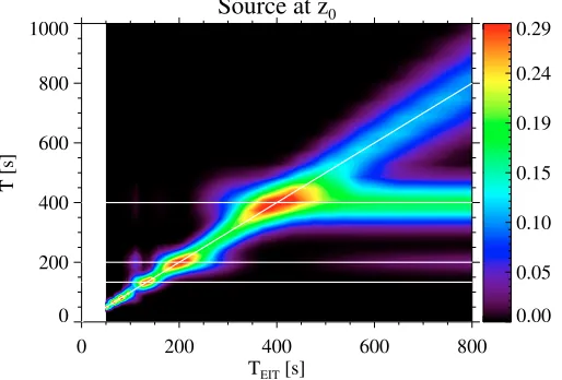
Source at z
00 200 400 600 800
TEIT [s]
0 200 400 600 800 1000
T [s]
[image:7.595.323.567.76.252.2]0.00 0.05 0.10 0.15 0.19 0.24 0.29
Fig. 2.The periods of oscillations generated by an EIT wave acting at
z = z0. The period of the driver is changed in the interval 50 to 800
s. The horizontal lines represent the natural periods of the loop, i.e.
Tn = 2π/ωn. The inclined line corresponds to the periods of the EIT wave, the driver of the oscillations in the coronal loop.
The pattern of oscillations which can be generated in the coronal loop depends on the characteristics of the driver. For each period of the driver (in between 50 and 800 s) a wavelet analysis has been carried out for the temporal part of Eq. (33). The power of the signal has been summed up inside the cone of influence set at a confidence level of 95% and the results are shown in Fig.2which is color-coded, the red color corresponds to the highest power, while the black color represents the lowest power. Depending on the period of the EIT wave, various oscilla-tion modes can be excited. For the example shown in Fig.2, the loop has a length of 200 Mm and a kink speed of 1000 km s−1. The natural periods corresponding to these values are in a ratio of 400/200/133, values represented by the horizontal lines.
Let us consider a driver which has a period larger than 600 s. In this case, the modes which can be excited will be the fun-damental mode (corresponding to 400 s) and the first harmonic but with a very low power. The oscillation pattern of the driver is still present but much weaker than the oscillation of the fun-damental mode. As the period of the driver becomes smaller, other harmonics can be excited. For a period between 200 and 400 s the pattern of the driver is preserved (see the inclined bright direction) but a considerable amount of the fundamental mode and first harmonic can be generated. Higher harmonics are also present but their power is very small. For a period of less than 200 s the dominant oscillations will be the first and second har-monics, while the fundamental mode is extremely weak. The red regions correspond to the cases when the period of the driver matches (or is very close) to one of the natural periods of the loop. In that case there is a resonance between the driver and the coronal loop.
In reality, however, if the EIT wave is an oscillating front colliding with the coronal loop, then the interaction occurs not only in one point, but in two, symmetrically situated from the ends of the loop. Let us suppose now that the driver is a front which interacts with the loopat the same timein two points, at z0and atL−z0. In this case, the driver will have the form
F =EEITλe
[δ(z−z0)+δ(z−L+z0)]e−λz ρi+ρe
eiωEITt.
Sources at z
0and L-z
00 200 400 600 800
TEIT [s]
0 200 400 600 800 1000
T [s]
0.00 0.05 0.10 0.14 0.19 0.24 0.29
Fig. 3.The same as in Fig. 2 but now the oscillations are generated by an EIT wave interacting with the coronal loop atz=z0andz=L−z0.
For this expression the resulting oscillations will be described by a similar function as given by Eq. (33) but now the spatial dependence will contain in the numerator the expression
eλz0sinα
nz0+e−λ(L−z0)sinαn(L−z0).
This situation can be achieved if the front of the EIT wave is per-fectly perpendicular to the coronal loop. For this particular driver the corresponding period-diagram is shown in Fig.3. According to expectations, in this case no modes corresponding to an even nwill be excited. In contrast to the first case, for driver’s period larger than the period corresponding to the first natural period (400 s) the EIT wave will excite modes which will carry predom-inantly the characteristic of the driver and in a smaller quantity the properties of the fundamental mode. No first harmonic can be generated, instead for a narrow range of the driver’s period, (a small interval around 200 s) the oscillations will comprise ad-dition from the fundamental mode and the second harmonic.
In reality it is more likely that the front of the incident EIT wave is not completely perpendicular to the axis of the loop, now the two interaction points between the loop and EIT wave will separated by a delay time, i.e. the time required for the front to reach the other half of the loop. The delay time can be easily calculated (see for details Ballai2007) and depends on the length of the loop, the speed of propagation of the EIT wave and the attack angle, i.e. the angle the front of the EIT wave makes with the vertical plane of the coronal loop. In this case, the acting force will have a spatial and temporal dependence of the form
δ(z−z0)eiωEITt+δ(z−L+z0)eiωEIT(t−Td)H(t−Td),
whereTdis the delay time andH(t) is the Heaviside step func-tion. After inserting this form back into Eq. (27) we obtain that the modified transversal displacement of the coronal loop is of the form
Q(z,t) = − 4EEITλe L3(ρ
i+ρe)
∞
n=1
sinαnz (ω2
EIT−ω2n)
×e−λz0sinα
nz0[cosωnt−cosωEITt]−e−λ(L−z0) ×sinαn(L−z0) [cosωn(t−Td)−cosωEIT(t−Td)]}.(34)
[image:7.595.48.305.79.253.2]T
delay= 2 T
EIT0 200 400 600 800
TEIT [s]
0 200 400 600 800 1000
T [s]
[image:8.595.34.282.77.253.2]0.00 0.05 0.10 0.15 0.20 0.24 0.29
Fig. 4.The same as in Fig.3but now the oscillations are generated by an EIT wave acting atz=z0andz=L−z0and the second interaction
is delayed by a time corresponding to the double of EIT waves’ period.
shown in Fig.4. It is obvious that the period of generated oscil-lations will contain the period of the EIT wave as the strongest component. For periods larger than the natural period of the fun-damental mode the generated oscillation will be dominated by the period of the fundamental mode with a weaker signal resem-bling the characteristics of the driver and a very weak period corresponding to the first harmonic. For periods of the driver situated between the natural periods of the loop, the possibility of mode generation goes parallel with the case explained in the case of a single driver. It can be easily shown that the distribution of possible periods in the coronal loop is similar even when the delay time is not an integer number of EIT waves’ period.
3.2. Non-harmonic driver
EIT waves have also been explained in terms of a non-wave feature (i.e. not having a harmonic behaviour). In this context we could list the models proposed by, e.g. Delanée (2000) and Attrill et al. (2007) where EIT waves were associated with de-formations and evolutions of magnetic fields resulted after the release of the CME. In order to include this possible explana-tion of EIT waves, let us suppose an external force acting on the coronal loop of the form
F =EEITλe
e−λzH(z−z
0)−H(z−z′0)
ρi+ρe
δ(t), (35)
which means that the external driving force is represented by a finite width (|z0−z′0|) front which has no temporal component other than a Dirac-delta function. If the form of external force given by Eq. (35) is inserted back into Eq. (27), we obtain that the temporal part of the transversal displacement of the magnetic tube modelling a coronal loop is given by
t
0
δ(t′) sinωn(t−t′)dt′∼sinωnt,
which means that this form of the EIT wave (a single finite width front) will produce oscillations in the coronal loop at the natural frequency of the loop only.
It is possible that the two forms of the external driver (the harmonic and non-harmonic) treated here coexist in the sense that they are the manifestation of the same phenomenon but at
different distance from the source, therefore a more careful anal-ysis will be needed in the future.
4. Conclusions
The generation and propagation of oscillations in coronal loops modelled by a straight magnetic cylinder with fixed ends is stud-ied when the coronal loop is under the effect of an EIT wave, as a driver. We found that if all forces acting on the flux tube are taken into account, the governing equation describing the propa-gation of standing transversal (kink) waves is described by an inhomogeneous Klein-Gordon-type equation and the inhomo-geneous part of the equation is represented by the force (over a unit volume) by EIT waves. The evolutionary equation con-tains information about the propagation speed of waves (here the kink speed) and the cut-offfrequency of kink modes. The cut-off value is determined by the densities inside/outside the loop and the Alfvén speed (i.e. magnetic field).
Using the combined Laplace and Fourier sine transform techniques, the governing equation is solved, such that the solu-tion takes into account general initial and boundary condisolu-tions.
Particular solutions have been found in the case of an EIT wave considered first as a wave with a frequencyωEIT, and later as a shock wave with finite front thickness (a non-harmonic driver). The results show that in case of a non-harmonic driver the periods of generated modes always belong to the natural pe-riods of the loop. On the other hand, in the case of a periodic driver – for an arbitrary period of the driver – there will be a mixture of standing modes which could explain on the observed period ratio. The analysis carried out here for different type of drivers show that the generated oscillations will carry predomi-nantly information about the driver rather than the loop itself.
The oscillations described in this paper were all modelled in the framework of ideal MHD. In reality coronal loop oscilla-tions are observed to decay relatively rapidly and several mech-anisms have been proposed to explain this damping (Ruderman & Roberts 2005; Terradas et al.2005,2007; Selwa et al.2007). The inclusion of a dissipative (or energy lost) mechanism in the present model will be addressed in a future study. It could be possible that in the case of a loop oscillating as a whole in the kink mode, the friction with the environment could be also an important factor whose inclusion in the model could result in a possible explanation of the damping of these oscillations.
The present study can be further extended to the case when the external EIT wave acts not only on a single magnetic loop but on a system of adjacent loops. In this case the primary displace-ment of the first coronal loop (generated by the incoming EIT wave) will be the driver for the oscillations in the second loop (and so on), leading to coupled loop oscillations. In order to de-scribe a realistic loop, the present model is going to be expanded to consider the effect of an external magnetic field. It is expected that the presence of this field will generate an additional force which will tend to suppress the oscillation of the tube.
Acknowledgements. I.B. acknowledges the financial support by NFS Hungary
(OTKA, K67746). I.B. and A.M. were supported by The National University Research Council Romania (CNCSIS-PN-II/531/2007). M.D. acknowledges the support from STFC.
References
Arregui, I., Terradas, J., Oliver, R., & Ballester, J. L. 2008, ApJ, 674, 1179 Aschwanden, M. J., Fletcher, L., Schrijver, C. J., & Alexander, D. 1999, ApJ,
1132 I. Ballai et al.: Forced oscillations of coronal loops driven by EIT waves
Attrill, G. D. R., Harra, L. K., van Driel-Gesztelyi, L., Démoulin, P., & Wüsler, J.-P. 2007a, Astron. Nachr., 328, 760
Attrill, G. D. R., Harra, L. K., van Driel-Gesztelyi, L., & Démoulin, P. 2007b, ApJ, 656, L101
Ballai, I. 2007, Sol. Phys., 247, 177
Ballai, I., Erdélyi, R., & Pintér, B. 2005, ApJ, 633, L145
Ballai, I., Erdélyi, R., & Hargreaves, J. 2006, Phys. Plasmas, 13, 042108 Banerjee, D., Erdélyi, R., Ramon, O., & O’Shea, E. 2007, Sol. Phys., 246, 3 Delanée, C. 2000, ApJ, 545, 512
Edwin, P., & Roberts, B. 1983, Sol. Phys., 88, 179 Erdélyi, R., & Hargreaves, J. 2008, A&A (in press)
Hargreaves, J. 2008, Ph. D. Thesis, University of Sheffield, 84 Hasan, S. S., & Kalkofen, W. 1999, ApJ, 519, 899
Hindman, B. W., & Jain, R. 2008, ApJ, 677, 899
Kalkofen, W., Rossi, P., Bodo, G., & Massaglia, S. 1994, A&A, 284, 976 Lamb,H. 1932, Hydrodynamics (Cambridge University Press), 138
Long, D. M., Gallagher, P. T., McAteer, R. T. J., & Bloomfield, D. S. 2008, ApJ, 680, 81
McEwan, M. P., Donnelly, G. R., Diaz, A. J., & Roberts, B. 2006, A&A, 460, 893
Musielak, Z. E., & Ulmschneider, P. 2001, A&A, 370, 541
Musielak, Z. E., & Ulmschneider, P. 2003, A&A, 400, 1057
Nakariakov, V. M., Ofman, L., DeLuca, E. E., Roberts, B., & Davila, J. M. 1999, Science, 285, 862
Rae, I. C., & Roberts, B. 1982, ApJ, 256, 761
Roberts, B. 2004, in Waves, oscillations and small-scale transient events in the solar atmosphere: a joint view from SOHO and TRACE, ESA SP-547, 1 Roberts, B., & Webb, A. R. 1978, Sol. Phys., 56, 5
Roberts, B., Edwin, P. M., & Benz, A. O. 1984, ApJ, 279, 857 Ruderman, M. S., & Roberts, B. 2002, ApJ, 577, 475
Selwa, M., Murawski, K., Solanki, S. K., & Wang, T. J. 2007, A&A, 462, 1127 Spruit, H.C 1981, A&A, 98, 155
Sutmann, G., Musielak, Z. E., & Ulmschneider, P. 1998, A&A, 340, 556 Terradas, J., Oliver, R., & Ballester, J. L. 2005, A&A, 441, 371 Terradas, J., Andries, J., & Goossens, M. 2007, Sol. Phys., 246, 231 Thompson, B. J., Gurman, J. B., Neupert, W. M., et al. 1999, ApJ, 517, 151 Verth, G., & Erdélyi, R. 2008, A&A, 486, 1015
Verth, G., van Doorselaere, T., Erdélyi, R., & Goossens, M. 2007, A&A, 457, 341
Verwichte, E., Nakariakov, V. M., Ofman, L., & Deluca, E. E. 2004, Sol. Phys., 233, 77