This is a repository copy of
Optimized Low Complexity Sensor Node Positioning in
Wireless Sensor Networks
.
White Rose Research Online URL for this paper:
http://eprints.whiterose.ac.uk/82376/
Version: Accepted Version
Article:
Salman, N, Ghogho, M orcid.org/0000-0002-0055-7867 and Kemp, AH (2014) Optimized
Low Complexity Sensor Node Positioning in Wireless Sensor Networks. IEEE Sensors
Journal, 14 (1). pp. 39-46. ISSN 1530-437X
https://doi.org/10.1109/JSEN.2013.2278864
[email protected] https://eprints.whiterose.ac.uk/
Reuse
Items deposited in White Rose Research Online are protected by copyright, with all rights reserved unless indicated otherwise. They may be downloaded and/or printed for private study, or other acts as permitted by national copyright laws. The publisher or other rights holders may allow further reproduction and re-use of the full text version. This is indicated by the licence information on the White Rose Research Online record for the item.
Takedown
If you consider content in White Rose Research Online to be in breach of UK law, please notify us by
Optimized Low Complexity Sensor Node
Positioning in Wireless Sensor Networks
Naveed Salman,
Student Member, IEEE,
Mounir Ghogho,
Senior Member, IEEE,
and A. H. Kemp,
Member, IEEE
Abstract—Localization of sensor nodes in wireless sensor networks (WSNs) promotes many new applications. Longer life time is imperative for WSNs, this requirement constrains the energy consumption and computation power of the nodes. In order to locate sensors at a low cost, the received signal strength (RSS)-based localization is favored by many researchers. RSS positioning does not require any additional hardware on the sensors and does not consume extra power. A low complexity solution to RSS localization is the linear least squares (LLS) method. In this paper, we analyze and improve the performance of this method. Firstly, a weighted least squares (WLS) algorithm is proposed which considerably improves the location estimation accuracy. Secondly, reference anchor optimization using a tech-nique based on the minimization of the theoretical mean square error (MSE) is also proposed to further improve performance of LLS and WLS algorithms. Finally, in order to realistically bound the performance of any unbiased RSS location estimator based on the linear model, the linear Cramer-Rao bound (CRB) is derived. It is shown via simulations that employment of the optimal reference anchor selection technique considerably improves system performance, while the WLS algorithm pushes the estimation performance closer to the linear CRB. Finally, it is also shown that the linear CRB has larger error than the exact CRB, which is the expected outcome.
Index Terms—Localization, Received signal strength (RSS), Cramer-Rao bound.
I. INTRODUCTION
W
IRELESS sensor networks (WSNs) consists of many small (up to several hundred) of low powered sensing nodes [1]. These nodes can be capable of sensing temperature, humidity, light intensity etc. In location aware WSNs, these nodes aside from sensing environmental conditions can also locate themselves. Thus promoting many new applications in the wireless communications industry. These applications may include firefighter tracking, cattle/wild life monitoring and logistics [2]. One way to locate the nodes is to use global positioning system (GPS), however deploying a GPS chip on every sensor node is expensive and energy consuming. Moreover, GPS assisted nodes can only be located when a guaranteed line of sight (LoS) is present with the navigational satellite. Hence nodes can be located using local positioning systems.Various techniques can be found in literature to locate wireless sensor nodes. Location algorithms, which are based on the absolute distance between nodes are known as range based algorithms. On the other hand, algorithms that do not require determining the actual inter-node distance for
The authors are with the School of Electronic and Electrical Engineering, University of Leeds, Leeds, U.K. M. Ghogho is also with International Uni-versity of Rabat, Morocco (e-mail: {elns, m.ghogho, a.h.kemp}@leeds.ac.uk).
localization are called range-free positioning algorithms [3], [4]. Range free algorithms are based on the number of hops for communications between two nodes as a distance metric. Range based algorithms are however more accurate than range free algorithms.
In the context of range based algorithm, distance can be estimated between nodes by making use of the angle of the impinging signal, this technique is more commonly known as the angle of arrival (AoA) technique [5], [6]. Apart from being very sensitive to errors due to multipath, AoA is not favored for low complexity WSN localization as an array of antennas or microphones are required on the sensor nodes to estimate the angle of the incoming signal. This increases the complexity and cost of the system. Absolute distance can be estimated using either the delay or attenuation of the signal. Systems capitalizing on the delay are more commonly known as time of arrival (ToA) systems. ToA localization, although more accurate, requires highly accurate clocks and hence are high in complexity [7], [8], [9]. On the other hand, received signal strength (RSS) based systems require no additional hardware and hence are more suitable for WSNs [10], [11], [12], [13]. For location estimation via RSS (and ToA) the so called trilateration technique is used. A number of nodes, usually high in resources and with known locations known as anchor nodes (AN) are used to estimate the locations of target nodes (TN). The location of ANs can be determined using GPS or they can be placed at predetermined positions. Readings from the TN is received at the ANs and are transmitted to a central station for processing.
Due to the non linear nature of the localization problem, location estimation via RSS (and also for ToA) can be achieved using maximum likelihood (ML) techniques [14], [15], [16] that commonly operate in an iterative fashion. Generally, a close initial estimate of location is required for the ML algorithm. Furthermore, the ML technique due to its iterative nature is high in complexity. On the other hand, location can also be estimated employing a low complexity linear least squares (LLS) approach [17].
2
degradation. Other techniques to linearize the system includes averaging the readings from all ANs and then pairing them with individual AN. Finally, pairing each AN with every other AN can be used for linearization. The system performance can be optimized by choosing an optimal reference AN and pairing it with all other ANs .
For ToA systems, the authors in [18] have formulated a technique to choose an optimal reference AN, however no such study has been done for RSS localization. In this paper we devise a technique for optimal reference AN selection using the RSS systems. In order to further improve the performance, the correlation between the (now linear) RSS readings is used and a weighted least squares (WLS) algorithm is proposed. For optimized performance the optimal AN selection for the WLS method is also given in the paper.
In order to compare the MSEs of estimators the Cramer-Rao bound has been extensively used as a benchmark. For ML algorithms, the CRB on location estimated has been derived for ToA in [19], [20] and for RSS systems in [12]. However, since the LLS method is note based on individual readings, the CRB given in [12] does not tightly bound the performance of the LLS-RSS estimator. For ToA LLS technique the CRB is given in [18]. In this paper we derive the linear CRB to tightly bound the performance of the LLS and WLS algorithm based on the RSS system.
To sum up, the main contributions of this paper are as follows:
• WLS algorithm for the linear model is proposed. • Optimal anchor selection for both LLS and WLS methods
is proposed.
• Linear CRB for RSS systems is derived.
Simulation results show that the linear CRB is significantly larger than the exact CRB and is thus more realistic in lower bounding the performance of RSS systems using the linear model. It is shown via simulations that the performance of the LSS estimator improves considerably when the optimal reference AN is used. The system performance is further improved using the WLS algorithm with optimal AN selection. The rest of the paper is organized as follows. Section II presents the problem statement and the system model. In Section III, the linear RSS model and the LLS solution is presented. In section IV, the WLS algorithm is proposed. In section V, the optimal reference AN selection technique is presented. In section VI, linear CRB is derived. Finally, in section VII, we discuss the simulation results which are followed by conclusions.
II. SYSTEMMODEL
For future use, we define the following notations.
Rn
is the set of ndimensional real numbers. T r(M) and
det(M)represent the trace and determinant of the matrix M
respectively. (.)T is the transpose operator.E(.)refers to the
expectation operator.(M)ijrefers to the element at theithrow
andjthcolumn of matrixM.N(µ, σ2)represents the normal
distribution with mean µ and variance σ2. 1N×N represents
the (N×N) matrix of all ones.
A two dimensional (2-D) network is considered, consist-ing of a TN which has unknown coordinates θ = [x, y]T
θ∈ R2
that are to be estimated, andM ANs with known locations θi = [xi, yi]T θi∈ R2 for i = 1, ..., M. The
received power at the ANs due to random shadowing is log-normally distributed. This model is based on empirical results obtained in [21], [22]. Thus the distancedi between the TN
and theithAN, is related to the path-loss at theithAN,Li,
and the path-loss exponent (PLE),αi, as [23]
Li =L0+ 10αilog
10di+wi, (1)
whereL0 is the path-loss at the reference distance d0 (d0<
di, and is normally taken as 1 m) and wi is a zero-mean
Gaussian random variable with known variance representing the log-normal shadowing effect, i.e. wi ∼ N 0, σi2
. The PLEs are assumed to be known via prior channel modeling or accurate estimation [25]. The path-loss is calculated as
Li = 10 log
10P−10 log10Pi (2)
whereP is the transmit power at the TN andPiis the received
power at the ithAN. The distance d
i is given by
di=
q
(x−xi)2+ (y−yi)2.
The observed path-loss (in dB) from d0 todi, zi =Li−L0,
can be expressed as
zi =fi(θ) +wi, i= 1, ..., M (3)
wherefi(θ) =γαilndi and γ = ln 1010 . In a vector form,
we have
z=f(θ) +w, (4)
wherez= [z1, ..., zM]T is the vector of the observed path
loss.f(θ) = [f1(θ), ..., fM(θ)]Tis the actual path-loss vector
andw= [w1, ..., wM]T is the noise vector.
Since the noise is Gaussian and assuming independence of the noise components, the joint conditional probability density function (pdf) ofzis given by
p(z|θ) =
M
Y
i=1
1
p
2πσ2
i
exp
(
−(zi−fi(φ)) 2
2σ2
i
)
. (5)
Thus, the maximum likelihood (ML) estimate of (5) is equivalent to the nonlinear least square (NLS) solution of the cost function
ε(θ) = (z−f(θ))T(z−f(θ)). (6) The solution to (6) is obtained using high complexity iterative techniques such as the Gauss-Newton or Levenberg-Marquardt techniques [15], [16]. Due to its iterative nature, the ML techniques can converge to local minimum instead of global minimum if given an initial seed that is far from the actual node location. Hence a close initial guess is essential to the reliability of the ML technique. In addition to the high complexity of the ML method, it can suffer from various other challenging issues detailed in [26].
can be estimated using a low complexity linear least squares technique explained in the next section.
III. LINEAR MODEL
The idea behind the LLS is to first linearize the RSS measurements and then use ordinary least squares (OLS) to estimate the unknown parameters. This idea was first intro-duced for ToA systems in [24] and analyzed for the same in [18]. However, for RSS measurements the the linearization is somewhat different due to additional parameters such as the PLEs. The non-linear system of path-loss equations can be linearized as follows. From (3), it can be readily shown that
E
1
βi
exp
2
zi
γαi
=d2i, whereβi = exp
2σ2
i
(γαi)2
. Similarly choosing a reference AN, it can be shown
E
1
βr
exp
2
zr
γαr
=d2r where βr = exp
2σ2
r
(γαr)2
. For linearization, the square of each distance equation is subtracted from the square of a reference distance equationd2r. This results in a linear system which is represented in matrix form as
b=Aθ+v, (7)
whereb= [b1, ..., bN]T,is the observation vector and is given
by
b=
δr−δ1−κr+κ1 δr−δ2−κr+κ2
.. .
δr−δN −κr+κN
for δr= β1rexp
2zr
γαr
andδi= β1iexp
2zi
γαi
. While
κr=x2r+y2randκi=x2i +yi2
for i6=r, i= 1, ..., N andN =M −1; andA is theN×2
data matrix
A= 2
x1−xr y1−yr
x2−xr y2−yr
..
. ...
xN−xr yN −yr
.
v is the noise vector which has zero mean and variance given by
ˇ
σi2=Eh δr−δi−d2r+d2i
2i
=d4iexp 4σ
2
i
(γαi)
2 !
−d4i +d4rexp 4σ
2
r
(γαr)
2 !
−d4r (8) and covariance
E
δr−δi−d2r+d2i
δr−δj−d2r+d2j
=
(
d4rexp 4σ
2
r
(γαr)
2 !
−d4r
)
. (9)
The solution to the LLS problem in is obtained by minimizing the cost function
εLLS(θ) = (b−Aθ)T(b−Aθ)
and is given as [27]
ˆ
θLLS=A†b, (10)
where A† is Moore–Penrose pseudoinverse i.e.
A†= (ATA)−1AT. The LLS can be implemented in
three different ways
1) LLS-ref: In this implementation, dr is the distance of
the TN from a reference AN as shown above.
2) LLS-avg: Instead of choosing a reference distance,dris
taken as the average of all distances from the ANs. Thus in this case,d2r= 1
N
PN
i=1d2i.
3) LLS-comb: In this case, combination of all pairs of ANs is considered and subtracted from each other. This results in M× M−1
2
equations. This technique is studied for ToA case in [28]. The elements of data matrix Aare now given by
A= 2
x1−x2 y1−y2
..
. ...
x1−xN y1−yN
x2−x3 y2−y3
..
. ...
xN−1−xN yN−1−yN
Similarly element of vector b are given as bij =
δi−δj−κi+κj
for for i, j = 1, ..., M and i < j. It should be noted that the number of equations increase considerably for large number of ANs. Hence LLS-comb is not favorable for large number of ANs.
We will compare the performance of all variants of the LLS algorithm in the simulation section.
IV. WEIGHTED LEAST SQUARES ALGORITHM
For the LLS solution obtained in (10), no knowledge about the reliability of each measurement is used. If this information is present, links that are more reliable are given more weigh-tage than others. Thus utilizing the information present in the covariance matrix, a weighted least square (WLS) algorithm is proposed in this section.
For a given covariance matrix C(θ) the WLS solution is obtained by minimizing the cost function
εW LS(θ) = (b−Aθ)TC(θ)−
1
(b−Aθ),
where the elements of C(θ) are given by (8) and (9). It is however noted that the elements of theC(θ)are dependent on the actual distance of the target node from the anchors, which is unknown, hence the estimated distance is used to estimated the covariance matrix Cθˆ. The WLS estimate is obtained as follows
ˆ
θW LS =A‡b‡, (11)
where A‡ =
AThCθˆi−1A−1AT and b‡ =
h Cθˆi
4
It is noted that similar to LLS, the WLS algorithm can also be implemented in three different modes i.e. ref, WLS-avg and WLS-comb. It is however seen that the covariance matrix is different for the three implementations. For WLS-ref, the diagonal and non diagonal terms of C(θ)are given by (8) and (9). For WLS-avg, where the reference anchor is the mean of all anchors, the M×M covariance is matrix is given below.
C(θ) = diagnd41exp
4σ2 1
(γα1)2
−d41+, ...,+d4Nexp
4σ2
N
(γαN)2
−d4No
+1M×M
(
d4rexp 4σ
2
r
(γαr)2
! −d4r
)
, (12)
where d4r = M1 PM
i=1d4i , σ2r =
1
M
PM
i=1σi2 and αr =
1
M
PM
i=1αi.
For the WLS-comb, development of the of theM22−M×
M2−M
2
covariance matrix becomes slightly complicated. As for WLS-ref and WLS-avg, the non-diagonal elements are same, however this is does now hold for WLS-comb for which the diagonal terms are given as
˜
σi2=Eh δi−δj−d2i +d2j
2i
=d4iexp 4σ
2
i
(γαi)2
!
−d4i +d4jexp 4σ
2
j
(γαj)2
!
−d4j (13) for i, j= 1, ..., M andi < j.
On the other hand, the non-diagonal terms are given by
E
δi−δj−d2i +d2j
δk−δl−d2k+d2l
for i, j= 1, ..., M andi < j andk, l= 1, ..., M andk < l
=
(
d4iexp 4σ
2
i
(γαi)2
! −d4i
)
fori=k.
=
(
d4jexp 4σ
2
j
(γαj)2
! −d4j
)
forj=l.
=− (
d4iexp 4σ
2
i
(γαi)2
! −d4i
)
fori=l.
=− (
d4jexp 4σ
2
j
(γαj)
2 !
−d4j
)
forj =k.
= 0 fori6=landj6=k.
V. OPTIMAL REFERENCE ANCHOR NODE SELECTION
Generally, the performance of LLS-avg and LLS-comb is slightly better than LLS-ref implementation due to the averaging effect of all ANs. Similarly, the performance of WLS-avg and WLS-comb is better than WLS-ref. However, in its basic form, LLS/WLS-ref randomly selects a reference AN. This could at times lead to degraded system performance as the accuracy of the location estimate depends on factors
such as the true distance dr from the TN, shadowing noise
variance σr2 and the PLEαr of a particular reference AN. In
this section, a technique to select the optimal reference AN is proposed. The optimal reference AN is chosen to be the AN that minimizes the MSE of the location estimates. Thus
θiopt = arg minθ i
(M SE). (16)
where
M SEθˆ=T r
E
ˆ
θ−θ0 θˆ−θ0
T
, (17)
whereˆθ is the estimated location via LLS or WLS andθ0
is the true location coordinates. The theoretical MSE is given for the LLS and WLS algorithm in the following subsections.
Theoretical MSE for LLS
For LLS, the estimated location ˆθ is given by ˆθLLS =
A†bwhile θ
0 can be represented byθ0 =A†b0, whereb0
represents the noise free observation vector and is given by
b0=
d2r−d21−κr+κ1 d2r−d22−κr+κ2
.. . d2
r−d22−κr+κN
.
Putting elements of θˆLLS and θ0 in (17) and after some
manipulation we obtain
M SEˆθLLS
=T r
A†K A†T ,
(18) where
K=EbbT−2E(b)bT0 +b0bT0
whereE(b) =b0. The diagonal and off diagonal elements
of EbbT are given by (14) and (15) respectively. Theoretical MSE for WLS
For the MSE of the WLS algorithm we use the estimated
ˆ
θW LS (11) in (17) to obtain the following MSE expression.
M SEθˆW LS
= T r
(
A‡C(θ)−1EbbT hC(θ)−1i
T
A‡T
−2hA‡C(θ)−1b0bT0 A† Ti
+hA†b0bT0 A† Ti
)
.
(19) It is noted that the theoretical MSE depends on the actual distances which are unknown, hence their estimates are used to estimate the MSE in (18) and (19). Once the optimal AN is selected, it is used again in the LLS solution (10) or WLS solution (11) to provide the final estimate of the TN location. This will be referred to as LLS-opt and WLS-opt respectively.
n
EbbTo
ii = κ
2
r + κ2i + d4
r
β2
r exp
8σ2
r
(γαr)2
+ d4i
β2
i exp
8σ2
i
(γαi)2
− 2d2r
βr exp
2σ2
r
(γαr)2
− 2d2i
βi exp
2σ2
i
(γαi)2
− 2κrκi −
2d2id2r
βiβr exp
2
σ2r
(γαr)2
exp 2σ2i
(γαi)2
+2d2rκi
βr exp
2
σ2r
(γαr)2
+2d2iκr
βi exp
2
σi2
(γαi)2
.
(14)
n
EbbTo
ij = κ
2
r + d4r
β2
rexp
8
σ2r
(γαr)2
− d2jd2r
βjβrexp
2σ2
j
(γαj)2
exp 2σ2r
(γαr)2
− d2id2r
βiβr exp
2
σi2
(γαi)2
exp 2σ2r
(γαr)2
+
d2
id2j
βiβj exp
2σ2
i
(γαi)2
exp 2σ2j
(γαj)2
− 2d2rκr
βr exp
2σ2
r
(γαr)2
+ d2rκj
βr exp
2σ2
r
(γαr)2
+ d2jκr
βj exp
2σ2
j
(γαj)2
+ d2rκi
βr exp
2σ2
r
(γαr)2
+
d2iκr
βi exp
2
σi2
(γαi)2
−d2iκj
βi exp
2
σ2i
(γαi)2
−d2jκ
βj exp
2σ2
j
(γαj)2
−κrκi−κrκj+κiκj.
(15)
Result 1. Equal PLEs and equal distances : In case of equal PLEs and equal distances of the TN from all ANs i.e αi=α,di=d∀i, the AN with the smallest noise variance
σi2is selected as the reference AN.
Result 2. Equal PLEs and equal noise variance : For equal PLEs and equal noise variance from all ANs i.e αi =
α, σ2i =σ2∀i, the AN with the shortest distancedi from the
TN is selected as the reference AN.
Result 3. Equal distance and equal noise variance: For equal noise variance and equal distances of the TN from all ANs i.eσ2
i =σ2, di=d∀i, the AN with the largest PLEαi
is chosen as the reference AN.
VI. PERFORMANCE BOUND
The CRB lower bounds the MSE performance of any unbiased estimator. For 2-D TN location, the CRB on the estimation MSE is given by
M SEθˆ≥ [I(θ)]11+ [I(θ)]22
det [I(θ)] , (20)
where [I(θ)] is the Fisher information matrix (FIM), and its elements are given by
[I(θ)]ij =−E
∂2lnp(p|θ)
∂θi∂θj
. (21)
To lower bound the ML algorithms, the elements of the FIM are given by
[I(θ)] =
PM
i=1
γ2α2
i(x−xi)2
d4
iσ2i
PM
i=1
γ2α2
i(x−xi)(y−yi)
d4
iσi2
PM
i=1
γ2α2
i(x−xi)(y−yi)
d4
iσ2i
PM
i=1
γ2α2
i(y−yi)2
d4
iσi2
.
(22) The CRB as obtained from the FIM in (22) only tightly bounds the performance of ML type algorithms. Since the LLS method is different from the ML approach, the exact CRB for RSS-based localization in [12] does not accurately predict the performance of estimators based on the linear model. Unlike the conventional CRB, which is based on the observations taken from individual ANs, the linear CRB is based on the observations
pi =
1 βr exp 2 zr γαr − 1 βi exp 2 zi γαi .
Clearly, β1 r,iexp
2
zr,i
γαr,i
represents a log-normal distribution; a closed form expression for the difference of two log-normal random variables is however not known. Although the summation of two log-normal random variables can be approximated by another log-normal random variable [29], [30],pi can be approximated by a Gaussian random variable
i.e.
pi∼N µiσˇ2i
where
µi=d2r−d
2
i (23)
and
ˇ
σi2=d4rexp 4σ
2
r
(γαr)
2 !
−d4r+d4iexp 4σ
2
i
(γαi)
2 !
−d4i. (24) In vector form,
p(p|θ)∼N(µ(θ),C(θ)), (25)
where µ(θ) = [µ1(θ), µ2(θ), ..., µN(θ)]T is the vector
constituting the means, and C(θ) is the N ×N covariance matrix whose elements are given by (9) and (12).
In order to prove the validity of the Gaussian assumption, the empirical cumulative distribution function (CDF) of pi
and the theoretical Gaussian CDF are plotted in Fig. 1. It is observed that even for a relatively large variance of σi2 = σr2 = 6, the empirical CDF closely fits the Gaussian CDF. The plot shows two cases, fordr> di and fordr< di.
It is clear that for both cases the Gaussian assumption holds true.
For the multivariate Gaussian distribution in (25), the ele-ments of the FIM are given by1
[I(θ)]ij =
∂µ(θ)
∂θi
T
C−1(θ)
∂µ(θ)
∂θj
+
0.5T r
C−1(θ)C(θ)
∂θi
C−1(θ)C(θ)
∂θj
. (26)
6
−80000 −6000 −4000 −2000 0 2000 4000 6000 0.1
0.2 0.3 0.4 0.5 0.6 0.7 0.8 0.9 1 1
pi
C
u
m
u
lat
iv
e
p
rob
ab
il
it
y
Empirical CDF dr= 50m, di= 40m
Theoretical Gaussian
dr= 50m, di= 40m
Empirical CDF
dr= 50m, di= 60m
Theoretical Gaussian
dr= 50m, di= 60m
Figure 1. Empirical CDF ofpiand theoretical Gaussian CDF.σ2i =σ2r= 6.
where
∂µi,j(θ)
∂x = 2 (x−xr)−2 (x−xi,j)
and
∂µi,j(θ)
∂y = 2 (y−yr)−2 (y−yi,j). (27)
The derivatives of C(θ)are given by (28) and (29).
VII. SIMULATION RESULTS
For performance comparison, we consider a circular de-ployment of 5 ANs around the origin of a 2-D coordinate system with radiusR. To evaluate the average performance at various TN positions, 20 TNs are randomly deployed inside the network. For simplicity, the noise variance associated with all ANs is kept the same i.e σ2
i = σ2r = σ2. A different
PLE value (given by vector α) is given to each AN, while the root mean square error (RMSE) is compared when the shadowing noise varianceσ2in the path-loss is increased. The simulations are run independently η times. The network AN and TNs deployment is shown in Fig. 2.
In Fig. 3, we analyze the performance of opt and LLS-ref. For LLS-ref, the RMSE is given while choosing each AN as a reference AN at a time for all 20 TNs. It is seen that the selection of some ANs as reference ANs exhibits better performance than others, this is primarily due to larger PLE value for that particular AN. However, since the simulations show the average performance for all 20 TNs, a larger PLE does not guarantee a particular AN to be an optimal reference AN, since it also depends on the actual distance from the TN. On the other hand, the performance of LLS-opt supersedes that of LLS-ref.
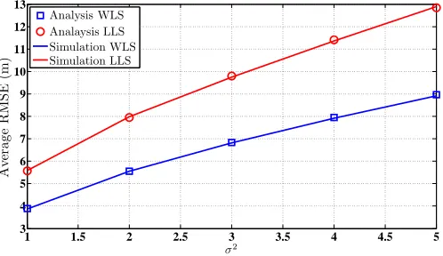
In Fig. 4, we compare the results obtained for the theo-retical MSE for LLS and WLS to the simulation for both algorithm respectively. It can be seen that that theoretical MSEs accurately predicts the performance of the LLS and WLS algorithms.
In Fig.5, performances of the variants of LLS and WLS are compared with LLS-opt and WLS-opt. The linear CRB is also plotted for comparison. For LLS-ref and WLS-ref, we randomly select AN-3 as the reference AN. As expected
−50 −40 −30 −20 −10 0 10 20 30 40 50 −50
−40 −30 −20 −10 0 10 20 30 40 50
X Axis
Y
Ax
is
Anchor Node
[image:7.612.55.562.57.200.2]Target Node
Figure 2. Network deployment
1 1.5 2 2.5 3 3.5 4 4.5 5 4
6 8 10 12 14
σ2
Av
er
a
g
e
R
M
S
E
(m
)
[image:7.612.59.565.60.389.2]AN 1 = Reference anchor AN 2 = Reference anchor AN 3 = Reference anchor AN 4 = Reference anchor AN 5 = Reference anchor LLS-opt
Figure 3. Performance comparison between LLS-ref for each AN as reference AN and LLS-opt. R = 50 m, η = 900, M = 5, α =
[2.4,2.6,2.8,3,3.2]T.
performance of avg and comb exceeds that of LLS-ref. However, the performance the LLS-opt surpasses all the other three LLS implementations. Interestingly, WLS-ref with reference AN-3 outperforms LLS-opt. However, the three variants of WLS algorithms perform similarly. While the WLS-opt performs better and approaches linear CRB.
1 1.5 2 2.5 3 3.5 4 4.5 5 3
4 5 6 7 8 9 10 11 12 13
σ2
Av
er
a
g
e
R
M
S
E
(m
)
Analysis WLS Analaysis LLS Simulation WLS Simulation LLS
Figure 4. Performance comparison between theoretical MSE for LLS and WLS with simulation. R = 50 m, η = 900, M = 5, α =
[image:7.612.313.562.558.702.2]∂C(θ)
∂x = diag
n
4d21(x−x1) h
exp 4σ12 (γα1)2
−1
i
+, ...,+4d2N(x−xN)
h
exp 4σ2N
(γαN)2
−1
io
+1N×N
n
4d2r(x−xr)
h
exp 4σr2
(γαr)2
−1
io
(28)
∂C(θ)
∂y = diag
n
4d21(y−y1) h
exp 4σ21 (γα1)2
−1
i
+, ...,+4d2N(y−yN)
h
exp 4σ2N
(γαN)2
−1
io
+1N×N
n
4d2r(y−yr)
h
exp 4σ2r
(γαr)2
−1
io
(29)
1 1.5 2 2.5 3 3.5 4 4.5 5 2
4 6 8 10 12 14
σ2
Av
er
a
g
e
R
M
S
E
(m
)
[image:8.612.49.299.177.316.2]LLS-ref LLS-avg LLS-comb LLS-opt WLS-ref WLS-avg WLS-comb WLS-opt Linear CRB
Figure 5. Performance comparison between different LLS and WLS implementations, linear CRB. R = 50 m, η = 900, M = 5, α =
[2.4,2.6,2.8,3,3.2]T.
1 1.5 2 2.5 3 3.5 4 4.5 5 3
4 5 6 7 8 9
σ2
Av
er
a
g
e
R
M
S
E
(m
)
Linear CRB Linear CRB-opt CRB
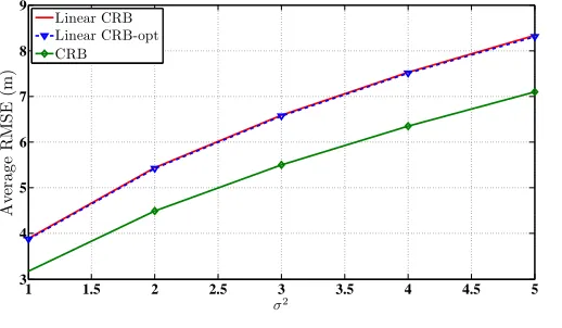
Figure 6. Performance comparison between linear CRB, linear CRB with optimal reference anchor and CRB. R= 50m, η = 900,M = 5,α=
[2.4,2.6,2.8,3,3.2]T.
In Fig.6, the CRB is compared with the linear CRB and as expected the performance the linear CRB shows larger error than the exact CRB. Thus the linear CRB is a more realistic bound for the linear RSS estimator. On the other hand, the linear CRB changed little with optimal reference anchor selection.
VIII. CONCLUSIONS
The RSS based LLS localization algorithm is a low com-plexity technique for node positioning for WSN positioning. In this paper, we have carried out a performance analysis and proposed improvements to the LLS method. The linear model was introduced and modified for three different LLS
variants. Performance was improved with a WLS algorithm that uses the information present in the covariance matrix of the observations. Further performance improvement was achieved with an optimal reference AN selection technique. The performance of the WLS method was shown to be close to the linear CRB which we have also derived. The linear CRB was shown to have larger error than the conventional CRB and thus realistically bounded the MSE of RSS location estimators operating on the linear model.
REFERENCES
[1] I. F. Akyildiz, W. Su, Y. Sankarasubramaniam, and E. Cayirci, “A survey on sensor networks,”IEEE Commun. Mag., vol. 40, no. 8, pp. 102–114, Aug. 2002.
[2] N. Patwari, J. N. Ash, S. Kyperountas, A. O. H. III, R. L. Moses, and N. S. Correal, “Locating the nodes: cooperative localization in wireless sensor networks,” IEEE Signal Processing Mag., vol. 22, no. 4, pp. 54–69, Jul. 2005.
[3] D. Niculescu and B. Nath, “DV based positioning in ad hoc networks,” Telecommun. Syst., vol. 22, no. 1, pp. 267–280, Jan. 2003.
[4] C. Savarese, J. Rabaey, and K. Langendoen, “Robust positioning al-gorithms for distributed ad-hoc wireless sensor networks,” in Proc. USENIX Tech. Annu. Conf., Jun. 2002, pp. 317–327.
[5] B.D. Van Veen and K.M. Buckley, “Beamforming: A versatile approach to spatial filtering,’’IEEE ASSP Mag., vol. 5, no. 2, pp. 4–24, Apr. 1988. [6] B. Ottersten, M. Viberg, P. Stoica, and A. Nehorai, “Exact and large sample ML techniques for parameter estimation and detection in array processing,’’ inRadar Array Processing, S.S. Haykin, J. Litva, and T. Shepherd, Eds. New York: Springer- Verlag, 1993, pp. 99–151. [7] A. H. Sayed, A. Tarighat, and N. Khajehnouri, “Network-based wireless
location,” IEEE Signal Processing Mag., vol. 22, no. 4, pp. 24–40, July 2005.
[8] S. Gezici, “A survey on wireless position estimation,”Springer Wireless Personal Communications, vol. 44, no. 3, pp. 263–282, Feb. 2008. [9] I. Guvenc and C.-C. Chong, “A survey on TOA based wireless
local-ization and NLOS mitigation techniques,”IEEE Commun. Surveys and Tutorials, vol. 11, no. 3, pp. 107–124, Aug. 2009.
[10] A. H. Sayed, A. Tarighat, and N. Khajehnouri, “Network-based wireless location,” IEEE Signal Processing Mag., vol. 22, no. 4, pp. 24–40, July 2005.
[11] P. Bergamo and G. Mazzini, “Localization in sensor networks with fading and mobility,” in Proc. IEEE Int’l Symposium on Personal, Indoor and Mobile Radio Communications, Sep. 2002, vol. 2, pp. 750-754. [12] N. Patwari, A. O. Hero, III, M. Perkins, N. S. Correal, and R. J. O’Dea,
“Relative location estimation in wireless sensor networks,”IEEE Trans. Signal Processing, vol. 51, no. 8, pp. 2137-2148, Aug. 2003. [13] R. Ouyang, A.-S. Wong, and C.-T. Lea, “Received signal strength-based
wireless localization via semidefinite programming: Noncooperative and cooperative schemes,” IEEE Trans. Veh. Technol., vol. 59, no. 3, pp. 1307– 1318, Mar. 2010.
[14] A. Rabbachin, I. Oppermann, and B. Denis, “ML time-of-arrival esti-mation based on low complexity UWB energy detection,” in Proc. IEEE Int. Conf. Ultrawideband (ICUWB), Waltham, MA, Sept. 2006. [15] X. Li, “RSS-Based Location Estimation with Unknown Pathloss Model,”
[image:8.612.52.311.373.524.2]8
[17] N. Salman, A. H. Kemp and M. Ghogho, “Low Complexity Joint Esti-mation of Location and Path-Loss Exponent”,IEEE Wireless Commun. Lett.-accepted for publication.
[18] I. Guvenc, S. Gezici, Z. Sahinoglu, “Fundamental limits and improved algorithms for linear least-squares wireless position estimation,”Wirel. Commun. Mob. Comput.(2010).
[19] Y. T. Chan, H. Y. C. Hang, and P. C. Ching, “Exact and approximate maximum likelihood localization algorithms,” IEEE Trans. Veh. Tech-nol., vol.55, no. 1, pp. 10–16, Jan. 2006.
[20] C. Cheng and A. Sahai, “Estimation bounds for localization,” in Proc.
IEEE Int. Conf. Sensor and Ad-Hoc Communications and Networks (SECON), Santa Clara, CA, Oct. 2004, pp. 415–424.
[21] H. Hashemi, “The indoor radio propagation channel,’’Proc. IEEE, vol. 81, no. 7, pp. 943–968, July 1993.
[22] T.S. Rappaport, Wireless Communications: Principles and Practice. Englewood Cliffs, NJ: Prentice-Hall, 1996.
[23] K. Pahlavan and A. Levesque, Wireless Information Networks. New York: John Wiley & Sons, Inc., 1995.
[24] J. J. Caffery, “A new approach to the geometry of TOA location,” in Proc.IEEE Veh. Technol. Conf. (VTC), vol. 4, Boston, MA, Sep. 2000, pp. 1943–1949.
[25] A. Bel, J. L. Vicario, and G. Seco-Granados, “Localization algorithm with on-line path loss estimation and node selection,”Sensors, vol. 11,
pp. 6905–6925, July 2011.
[26] G. A. F. Seber and C. J. Wild, Nonlinear Regression. Hoboken, NJ: Wiley-Interscience, 2003.
[27] S. M. Kay,Fundamentals of Statistical Signal Processing: Estimation Theory. Upper Saddle River, NJ: Prentice Hall, Inc., 1993.
[28] Venkatesh S, Buehrer RM. A linear programming approach to NLOS error mitigation in sensor networks. In Proceedings of IEEE Inter-national Symposium on Information Processing in Sensor Networks (IPSN), Nashville, Tennessee, April 2006; 301–308.
[29] Jingxian Wu, N.B. Mehta, Zhang Jin, "Flexible lognormal sum ap-proximation method," Global Telecommunications Conference, 2005. GLOBECOM ’05. IEEE, vol.6, no., pp.3413-3417, 2-2 Dec. 2005. [30] L. Fenton, "The Sum of Log-Normal Probability Distributions in Scatter
Transmission Systems,"IRE Transactions onCommunications Systems,