This is a repository copy of
Parallel centerline extraction on the GPU
.
White Rose Research Online URL for this paper:
http://eprints.whiterose.ac.uk/150787/
Version: Accepted Version
Article:
Liu, B., Telea, A.C., Roerdink, J.B.T.M. et al. (6 more authors) (2014) Parallel centerline
extraction on the GPU. Computers & Graphics, 41. pp. 72-83. ISSN 0097-8493
https://doi.org/10.1016/j.cag.2014.02.003
Article available under the terms of the CC-BY-NC-ND licence
(https://creativecommons.org/licenses/by-nc-nd/4.0/).
[email protected]
https://eprints.whiterose.ac.uk/
Reuse
This article is distributed under the terms of the Creative Commons Attribution-NonCommercial-NoDerivs
(CC BY-NC-ND) licence. This licence only allows you to download this work and share it with others as long
as you credit the authors, but you can’t change the article in any way or use it commercially. More
information and the full terms of the licence here: https://creativecommons.org/licenses/
Takedown
If you consider content in White Rose Research Online to be in breach of UK law, please notify us by
This is a repository copy of
Parallel centerline extraction on the GPU
.
White Rose Research Online URL for this paper:
http://eprints.whiterose.ac.uk/150787/
Version: Accepted Version
Article:
Liu, B, Telea, AC, Roerdink, JBTM et al. (6 more authors) (2014) Parallel centerline
extraction on the GPU. Computers & Graphics, 41. pp. 72-83. ISSN 0097-8493
https://doi.org/10.1016/j.cag.2014.02.003
eprint
[email protected]
https://eprints.whiterose.ac.uk/
Reuse
Items deposited in White Rose Research Online are protected by copyright, with all rights reserved unless
indicated otherwise. They may be downloaded and/or printed for private study, or other acts as permitted by
national copyright laws. The publisher or other rights holders may allow further reproduction and re-use of
the full text version. This is indicated by the licence information on the White Rose Research Online record
for the item.
Takedown
If you consider content in White Rose Research Online to be in breach of UK law, please notify us by
Parallel Centerline Extraction on the GPU
Baoquan Liu1, Alexandru C. Telea2, Jos B.T.M. Roerdink2, Gordon J. Clapworthy1,
David Williams2, Po Yang1, Feng Dong1, Valeriu Codreanu2,3and Alessandro Chiarini4
1University of Bedfordshire 2University of Groningen 3Eindhoven University of Technology 4SCS srl
Abstract—
Centerline extraction is important in a variety of visualization applications including shape analysis, geometry processing, and virtual endoscopy. Centerlines allow accurate measurements of length along winding tubular structures, assist automatic virtual navigation, and provide a path-planning system to control the movement and orientation of a virtual camera.
However, efficiently computing centerlines with the desired accuracy has been a major challenge. Existing centerline methods are either not fast enough or not accurate enough for interactive application to complex 3D shapes. Some methods based on distance mapping are accurate, but these are sequential algorithms which have limited performance when running on the CPU. To our knowl-edge, there is no accurate parallel centerline algorithm that can take advantage of modern many-core parallel computing resources, such as GPUs, to perform automatic centerline extraction from large data volumes at interactive speed and with high accuracy. In this paper, we present a new parallel centerline extraction algorithm suitable for implementation on a GPU to produce highly accurate, 26-connected, one-voxel-thick centerlines at interactive speed. The resulting centerlines are as accurate as those produced by a state-of-the-art sequential CPU method [40], while being computed hundreds of times faster. Applications to fly-through path planning and virtual endoscopy are discussed. Experimental results demonstrating centeredness, robustness and efficiency are presented.
Index Terms—Centerline, parallel algorithm, GPU techniques, virtual endoscopy.
1 INTRODUCTION
Centerlines are powerful descriptors of 3D shapes that exhibit local circular symmetry [12]. Biomedical shapes that are effectively de-scribed by centerlines include blood vessels, intestines, and airways. In this context, centerlines are useful for virtual navigation, such as virtual endoscopy using the colon centerline to control the movement and orientation of the virtual camera. Accurate length measurements and navigation through other tubular organs, such as the aorta or coro-nary arteries [30], also require centerline computations. The problem of finding the optimal paths of minimal collision probability for vir-tual engineering and architectural applications also involves center-lines [17].
Although the concept of a centerline is quite intuitive, its math-ematical definition is not unique. The concept of a centerline (also known as a medial or symmetry axis) was first introduced by Blum [10]. Based on previous work [3, 7, 8, 12, 39, 40], an adequate center-line definition should meet at least the following three requirements: Connectivity, Centerednessand Singularity. Connectivity requires that the centerline of a compact shape is also a compact object. For sampled objects, such as voxel models, this implies that centerlines of compact objects are sets of connectedvoxels. Centeredness re-quires that the centerline should be locally centered within the input shape with respect to the object boundary. Singularity requires that the centerline should be a single 1D path with no branches or self-intersections, and as thin as the sampling representation permits. For volumetric data, centerlines should be one voxel thick. A further re-quirement that there be no self intersections is desirable for some ap-plications, such as path planning in virtual endoscopy.
Centerlines are closely related, but not identical to, other shape de-scriptors such as surface and curve skeletons. Unlike a centerline, the surface skeletonS of a 3D shapeΩ⊂R3is uniquely defined as the locus of the centers of maximally-inscribed 3D spheres inΩ[3, 27]. This results in 3D surfaces or 2D manifolds. In contrast to surface
Manuscript received 31 March 2007; accepted 1 August 2007; posted online 27 October 2007.
For information on obtaining reprints of this article, please send e-mail to: [email protected].
skeletons,curve skeletonsCare loosely defined as 1D structures with
branches, which are locally centered within, and homotopic with, the input shape Ω. The lack of a universally accepted formal defini-tion has led to a situadefini-tion in which the various methods that compute curve skeletons use different definitions and thus produce differing re-sults [3, 4, 27, 30, 37].
Centerlines share features such as centeredness, connectivity and 1D dimensionality with curve skeletons. However, unlike a curve skeleton, acenterlineL is typically defined as a single path with no
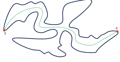
branches or self-intersections. An additional requirement is that a cen-terline passes through two user-selected end pointsS∈∂Ω,E∈∂Ωon the surface∂Ωof the objectΩ[7, 8, 39, 40]. This allows users to con-fine the extracted centerline to only a desired part of the shapeΩ,e.g., for a controlled measurement of a branchless 1D fly-through path. An example centerline is shown in Fig. 1; while the two end points can be arbitrarily chosen on the object surface by the user (or be detected au-tomatically, too), the resulting centerline between them quickly tends towards the local center of the object.
S
[image:3.612.329.534.523.630.2]E
Fig. 1. An example centerline connecting two user-defined endpoints (source and end points), which allow a particular segment of the object to be specified for fly-through path planning.
In summary, the difference between a centerline L and a curve
skeletonC lies in two aspects: (1) a centerline is a single path with
deter-mined simply by the object’s shape.
Hence, while a curve skeleton is fully locatedinsidethe object (ex-cept for some special cases, such as 1- or 2-voxel wide parts of objects which cannot be traversed by a voxel-thick curve without touching the surface∂Ω), a centerline must start from, and end on, the surface ∂Ω. As a compact representation of an object’s topological structure, a curve skeleton is well suited to 3D animation, morphing, match-ing and registration [13]. In contrast, centerlines are more useful in visualization applications such as fly-through path planning between user-specified end points.
Ideally, a centerline extraction algorithm should generate a good approximation to the central path through a shapeΩ,i.e., the center-lineL should be as close as possible to the corresponding parts of the curve skeletonC ofΩ, apart from in the regions close to whereL
connects to its endpoints on∂Ω. Centerlines should be computable at interactive rates even for large and complex objects sampled at high resolutions. This last constraint is especially important when consider-ing the potential deployment of centerlines in a clinical environment, where interactive performance is highly desirable. For instance, a re-cent detailed evaluation of the quality of re-centerlines used for coro-nary artery exploration considered 14 centerline extraction methods deemed suitable, from an accuracy perspective, for medical applica-tions [30]. Typical running times of these methods range between tens of seconds and hours per dataset, which clearly makes them unsuitable for interactive exploration.
In virtual colonoscopy, centerline extraction provides a compact colon shape description and enables accurate colon geometry mea-surement for both pre-planned and interactive navigation. During treatment, problems involved in issues such as precise polyp regis-tration between virtual and “real” fiber-optic colonoscopy or shape registration between supine and prone CT scans can be overcome by using centerlines. However, extracting centerlines from large voxel volumes while satisfying centeredness, singularity, and computational efficiency remains very challenging.
Many methods have been proposed for the computation of center-lines, either from 3D (CT or MRI) [30] scans or from 3D polygonal models [36]. The most efficient and accurate centerline extraction method is considered to be that based on Euclidean distance map-ping [7, 8, 39, 40]. Here, centerline points are forced to lie as far from the object boundary as possible by the use of a distance-from-boundary (DFB) field. This ensures that the centerline is a subset of the surface skeletonS, which is located along the DFB maxima [27].
However, this method is a canonical serial algorithm with fundamental dependency between iterations. It does not readily lend itself to paral-lelization as it relies on a sorted priority queue and can evaluate only one voxel (i.e., the head of a queue) for each iteration. As a result, the algorithm cannot take advantage of the multiple parallel comput-ing cores now available on the CPU or GPU, as discussed further in Section 3.
The main contribution of this paper is a new parallel centerline ex-traction algorithm suited to modern GPU hardware. Our algorithm adopts the general DFB-based centerline extraction approach [40], which is regarded as state of the art. However, instead of evaluat-ing the nodes serially, we propose that multiple node-evaluations are performed concurrently on parallel computing cores by using a paral-lel wavefront propagation technique. This allows the new algorithm to be implemented in a parallel GPGPU environment. Our experiments have shown that the proposed GPU algorithm produces an accurate centerline with the same quality as the original algorithm, but it runs hundredsof times faster, thus allowing centerline extraction to be per-formed at interactive rates. This level of interactivity makes a funda-mental difference to the way in which applications such as virtual path planning can be performed.
2 RELATEDWORK
The problem of centerline extraction has received a great deal of at-tention over many years, and a vast number of centerline calculation algorithms have been described in the literature.
The earlymanual markingmethod [15] requires intensive manual
intervention as the user has to indicate key points at the center of each object region on each of the several hundred axis-aligned 2D slices of a volume dataset. The algorithm then computes the centerline curve by interpolation. This method is simple, but time-consuming and te-dious in operation, and its results are by no means more accurate than those produced by automatic methods. Because the colon is usually visualized on a 2D screen, it is difficult for users to locate points that are centered inside it, so this method is highly liable to human error.
Topological thinningmethods remove voxels on the boundary∂Ω while preserving connectivity and topology [6, 24]. Voxel removal in distance-to-boundary order enforces centeredness [3, 26]. The result-ing structure, typically either the surface skeletonSor curve skeleton
C ofΩ, can next be simplified, or pruned, in order to extract the de-sired centerlineL [28]. Although the thinning procedure is
conceptu-ally simple, its requirement for a distance-driven ordering, topological checking and postprocessing, can make the entire procedure quite in-tricate and time-consuming [3]. A 3D thinning implementation for ITK by Homann [19] is quite popular in the medical imaging commu-nity.
Voronoi diagram methods [1] find centerlines as the paths in Voronoi diagrams that minimize the integral of the radii of the maxi-mal inscribed spheres along the path; this is equivalent to finding the shortest paths in the radius metric. To perform the calculation, a wave is propagated from a source point (one centerline end point) using the inverse of the radius as the wave speed, and the wave arrival time is recorded at all points of the Voronoi diagram; the line is then back-traced from a target point (the other end point of the centerline) along the gradient of the arrival times. The propagation can be described using the Eikonal equation and is computed using the fast marching method [32]. This method was implemented in the Vascular Modeling Toolkit (VMTK) [2], but this has only a CPU version. This method is accurate but too slow for interactive application. Indeed, computing an accurate Voronoi diagram of the input shape is equivalent to com-puting its surface skeletonS, and this computation is not interactive, even in recent GPU implementations [20, 22].
Distance mappingapproaches were first used in robotic path plan-ning [21]. They are generally considered to provide the fastest solution among the different categories. Such methods have two phases. The first phase computes the distance from a user-specified source point Sto each voxel inside the 3D object, called the DFS (distance from source) map. In the second phase, the shortest path from the other end pointEto the source point is found by descending through the gradi-ent of the DFS map. The shortest path can be rapidly extracted by a simple backtracing. Conceptually and algorithmically, this approach is essentially the same as the method for computing geodesics between two given points on a surface [25].
Previous centerline algorithms using distance mapping differ in how they specify the distances between orthogonal, 2D-diagonal, and 3D-diagonal neighboring voxels. The most accurate distance measure is the Euclidean metric, but most algorithms use approximate distance transformation metrics such as the Manhattan metric [7, 8, 39, 40] in order to reduce the computational cost. Distance mapping approaches often employ Dijkstra’s shortest path algorithm on the voxel connec-tivity graph to extract the centerline fully automatically.
Although distance mapping can meet the connectivity and singu-larity criteria well, in many implementations its centeredness is of-ten less than perfect as the resulting path of-tends to ‘hug’ the concave corners of∂Ωat sharp turns (i.e., the tendency of the centerlineL
and effectively by employing the DFB field as node-weights and ex-tracting the centerline from a minimum-cost spanning tree (MST) built from the DFB field. This efficient and robust algorithm is fully auto-matic and can generate accurate centerlines, but it has three properties inhibiting parallelization: a fundamental loop dependency, limited ex-plicit parallelism, and excessive synchronization. We discuss these issues further in Section 3.
Level setmethods [16,38] have been found to produce accurate cen-terlines. However, they are not fast enough for interactive applications. Smistadet al.[35] introduced an efficient GPU-based airway tree segmentation algorithm that extracts centerlines by performing a ridge traversal on the result of a tube detection filter. The ridge traversal approach, first proposed by Aylwardet al.[5], is performed on filtered images, so it can have accuracy problems due to its sensitivity to noise, local artifacts and its initialization, as mentioned in [33, 35]. Also, this algorithm remains completely serial in form, so it is difficult to increase its speed by GPU parallelization.
Recently Smistadet al. [34] introduced a new model-based Tube Detection Filter (TDF) combined with a new parallel centerline algo-rithm which can extract centerlines directly from the TDF result. Their results show that the method is able to extract airways and vessels in 3– 5 seconds on a high-end GPU, and their parallel centerline extraction algorithm is 1–2 seconds faster than the serial ridge traversal extrac-tion algorithm.
Several voxel-based methods have been proposed to compute Eu-clidean surface and/or curve skeletons of 3D data [3, 4, 14, 18, 27]. A recent qualitative comparison of curve skeleton techniques is given in [36]. However, these methods do not produce single-path center-lines between user-specified endpoints. It is conceivable that such methods could be post-processed to extract centerlines, for example by finding the shortest-path linking the specified endpoints which also passes through an extracted curve skeleton. However, none of these methods is fast enough for near-real-time curve skeletonization of large 3D volumes, and the postprocessing could be tedious and time-consuming, so they fail our interactive requirement.
Bleiweiss [9] introduced a GPU implementation of parallel pathfinding for many thousands of agents in crowded game scenes in which each individual agent runs a separate pathfinding algorithm (to find its own individual path) in a single GPU thread. Therefore, the parallelism lies in the multiple agents’ multiple pathfindings, which is a coarse granularity parallelism. In contrast, our parallel algorithm ex-hibits fine granularity parallelism, with multiple GPU threads working together to find a single path for a complex-shape object.
[image:5.612.50.289.514.652.2]3 REVIEW OF THE SERIAL ALGORITHM
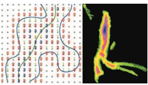
Fig. 2. Examples of DFB shown in 2D slices. Left: explicit DFB values; right: an aorta DFB field visualized through a color map (image courtesy of Bitter et al. [7]).
In this section, we first review the serial algorithm introduced by [40]; this will be referred to hereafter asserial). Our new parallel algorithm is then introduced incrementally in the following sections.
In the serial algorithm, the centerline is defined as the minimum-cost path spanning the 3D DFB field inside the input object. An ex-ample DFB field is shown in Fig 2. This is a concise and concrete definition, similar to the traditional centerline description given by Blum [10], but it is more practical for implementation. The serial al-gorithm can produce very accurate centerlines based on the DFB field, in which the Euclidean distance between each interior voxel and the object boundary is recorded.
The serial algorithm consists of two main steps. First, it builds a minimum-cost spanning tree (MST) in the DFB field, then it finds the sequence of voxels that lie along the centerline by backtracing from the end point to the start point through the previously constructed MST. The first step is by far the costlier in terms of computation. Centered-ness is assured by the fact that the DFB field uses exact Euclidean distances, computed by a fast algorithm proposed by Saitoet al.[29] and described also by Meijsteret al.in [23].
The serial algorithm solves the centerline problem on graphs with nonnegative edge weights by looping over the contents of a priority queue until all nodes have been evaluated. The regular sampling grid of the DFB field is treated as a 3D directed weighted graph. Each voxel corresponds to a graph node. Graph edges are given by the 26-neighbor relations between adjacent voxels. Each edge has two directions pointing towards its two respective end points, and each di-rection has its own weight, called the DFB-cost, equal to the inverse of the DFB of the end voxel to which it points.
The MST is defined as a tree that connects all of the interior voxels (that is, those inΩ\∂Ω) at the minimum DFB-cost. To build this MST efficiently, a modified Dijkstra technique is used. Given a source point Sand an end pointE, both specified interactively by the user on the object surface∂Ω, the MST is built by the following four-step process:
1. MarkSas visited and define it as the current nodeC. Set the pathlinkofSto NULL, wherepathlinkis used to label a node’s predecessor in a path.
2. For the current nodeC, insert the unmarked 26-neighborsBof Cinto a priority queueQsorted on the DFB-cost, and set their pathlinks toC.
3. Remove the head node fromQ(that is, the one with the minimum DFB-cost), mark it as visited, and define it as the current nodeC.
4. Repeat from step 2 untilQis empty. After this, all nodes have been evaluated.
The algorithm constructs, for each interior voxelp∈Ω\∂Ω, a path-link pointing toward its neighboring voxels, through whichpreaches the source pointSwith a minimum DFB-cost. At each iteration, the priority queue must be kept sorted (either by explicit re-sorting or by ensuring that any insertion retains the overall ordering) in order to find the nodeCthat has the minimum DFB-cost. This node is used to launch the next iteration, which will, in turn, insert new nodes (i.e., C’s neighbors) into the queue.
The above algorithm is completely serial, and its speed cannot be increased by the use of parallel hardware due to the fundamental loop dependency caused by the use of a priority queue. Specifically, to en-sure a correct MST construction, based on the greedy rule that infor-mation is propagated only from the node with theminimumDFB-cost to other nodes at any time, only a single node can be processed at each iteration to update its 26 neighbors. Furthermore, processing the node Cat the head of the queue causes its neighbors to be inserted into the queue which, in turn, requires the queue to be re-ordered to ensure that the minimum DST-cost node is at the front.
This process exhibits excessive synchronization: at every iteration only the head node can be processed, and each node-evaluation has to wait for the completion of the sorting operations from the last itera-tion, so multiple node evaluations cannot be performed concurrently. Apart from the above, a further bottleneck is presented by the frequent sorting of the queue. Each sorting operation is performed at best in O(logM), whereMis the average number of elements in the priority
queue at each iteration. Moreover, the total number of iterations we need to loop in this algorithm is equal toK=Ω, the number of the foreground voxels inside or on the 3D shapeΩ(rather thanN,i.e., the total number of voxels in the volume), since allKvoxels need to be removed from the queue (one at each iteration) in order to propagate information throughout the object. So the complexity of the whole algorithm isO(K×logM).
4 QUEUE-FREE SERIAL ALGORITHM RUNNING ON THECPU
As a first step towards parallelization, we introduce in this section a queue-free serial algorithm running on the CPU based on the same DFB field as the original serial algorithm in Sec. 3. In the following sections, we show how we parallelize this queue-free algorithm for the GPU by allowing parallel evaluations of multiple nodes.
As explained in Sec. 3, the original serial algorithm [40] is not parallelizable due to its fundamental loop dependency, which is caused by the use of a priority queue. To bypass this problem, here we first introduce a new brute-force serial algorithm (referred to asb f s) which does not use a priority queue. This new queue-free algorithm is based on the same accurate Euclidean DFB field asserialand again assumes that the object interior is a 26-connected region. The DFB field is stored as a signed floating-point distance field, that is, it has positive values for voxels inside∂Ω, zero values on∂Ω, and negative values outside∂Ω.
The DFB-cost field is stored as a 3D read-only volumeDFBcost.
A second 3D floating-point buffer,weight, is used to store, for each voxel, the accumulated weight value along its path originating from S. Each element ofweight is initialized to a very large constant, MaxFloat, except the source pointS, whoseweight[S]is set to 0. As the algorithm proceeds, we compute the accumulated weight from a source pointSto each of its neighborsBusing the formulaweight[B] = weight[S] +DFBcost[B]. The neighbor nodes then propagate their
weight values progressively to their own neighbors untilEis reached. To construct a correct MST, our new algorithm ensures that the weightvalues are propagated only from nodes with smaller weights to nodes with larger weights. Thus, the weight values of individual nodes can only decrease monotonically as a result of the node evaluations – during the iterations, all node weights (exceptS) will be updated from MaxFloat to smaller values in a monotonically decreasing manner. In this way, the MST can be constructed in a “downwind” direction proceeding from the source pointSto the end pointE.
Algorithm 1Queue-free serial algorithm (b f s)
1: blue// input:DFBcost,S; 2: blue// output:weight;
3:
4: blue// Initialization:
5: SetMemory(weight,MaxFloat); blue//set all memory toMaxFloat
6: weight[S] =0;
7: bFinished=0;
8:
9: blue//iteration loop:
10: whilebFinished==0do
11: bFinished=1;
12: forC=0 toN−1do// iterating on allNvoxels
13: ifweight[C]<MaxFloatthen
14: foreach neighborBofCdo// iterating on all 26 neighbors ofC
15: ifDFBcost[B]>0then
16: newWeight=weight[C] +DFBcost[B]; blue//potential new weight ofB
17: ifnewWeight<weight[B]then
18: weight[B] =newWeight; blue//updating weight
19: bFinished=0;
20: end if
21: end if
22: end for
23: end if
24: end for
25: end while
The pseudo-code ofb f sis shown in Algorithm 1. In detail, we proceed as follows:
1. At initialization, the source pointSis selected by the user, and weight[S]is set to zero. A Boolean value (bFinished), used to indicate termination, is also set to 0.
2. At each iteration, ifbFinished==0, we reset it to 1, and then launch a for-loop to iterate on allN voxels of the input vol-ume. Here, we propagate the weight information from each vis-ited voxelCto its 26-neighbors. Each neighborBofChas its weight[B]value updated toweight[C] +DFBcost[B]if this value
is smaller thanweight[B], which ensures thatweight[B]can only decrease. If any weight update is successful, we setbFinishedto 0, which means we need next to propagate information fromB to its own neighbors at the next iteration.
3. Step 2 is repeated until no further weight updates occur (bFinished=1). At this point, the final MST is available in the weightdataset.
The number of iterations is bounded because, after the propagation has reached all of the interior nodes and no weights remain to be up-dated, the iteration procedure will terminate.
At each iteration, this algorithm evaluatesNvoxels, whereNis the total number of voxels in the input 3D volume, whereasserial eval-uates only the nodes that were removed from its priority queue. The number of these nodesK=Ω, that is, the voxels on or inside the 3D shape (i.e., the foreground voxels). As a result, our brute-force algo-rithmb f sis slower thanserial, sinceK<N, sob f sis uncompetitive on a serial processor.
However,b f sis queue free and has no loop dependency. As such, it is completely parallelizable, leading to the possibility of a highly-efficient GPU-based centerline extraction method, as discussed in the next section.
We also note that the centerlines produced by theserialandb f s al-gorithms may be slightly different as the respective MSTs are created in slightly different ways. Inb f s, the weight values are not explic-itly sorted, but are accumulated (weight[C] +DFBcost[B]) and updated
in a monotonically decreasing manner. The final path connecting the source to destination nodes is found by tracing paths in the gradient of the accumulated weight field. In contrast,serialsorts the weights explicitly (but does not accumulate them), and uses a pathlink to con-nect the sorted nodes after the weight-ranking to construct the MST. The differences in the MSTs are very small and lead to insignificant centerline differences, as we show in Sec. 6.
5 GPUPARALLELIZATION
We next present two parallel implementations of theb f salgorithm using the GPU. The key idea behind both implementations is to al-low multiple node evaluations to be performed concurrently using the many computing cores available on a GPU. Both implementations store theDFBcostfield as a 3D GPU texture. After the MST is
con-structed in parallel on the GPU, we transfer it to the CPU, where we construct the final centerline by simply backtracking in the MST from the endpointEto the starting pointS.
The first implementation (b f p, Sec. 5.1) is a brute-force paral-lelization, which is simple to implement, while the second implemen-tation (im p, Sec. 5.2) is more involved, but considerably more effi-cient. Both produce results identical to those ofb f s.
5.1 Brute-force parallel algorithm
The brute-force parallelizationb f pis a direct mapping of the queue-free serial algorithmb f sonto the GPU, where we evaluate allN vox-els of the input volume in parallel at each iteration. The pseudo-code ofb f pis shown in Algorithm 2. In detail, we proceed as follows:
2. At the beginning of each iteration, ifbFinished==0, we reset it to 1, and then launch a CUDA kernel in exactlyNGPU threads. The thread associated with nodeCpropagates the weight infor-mation fromCto its 26-neighbors. To ensure that the weight of any neighbor Bcan only decrease, we use CUDA’s atomic functionatomicMin(). If an update ofBis successful, we set bFinishedto 0. The iterations are repeated untilbFinished=1 at the end of an iteration.
Algorithm 2Brute force parallel algorithm (br p)
1:blue// input:DFBcost,S; 2:blue// output:weight;
3:
4:blue// Initialization:
5:SetMemory(weight,MaxFloat); blue//set all memory toMaxFloat
6:weight[S] =0;
7:bFinished=0;
8:
9:blue//iteration loop:
10: whilebFinished==0do
11: bFinished=1;
12: call the CUDA kernel BruteForceParallelIterationKernel(N); blue//this launchesNparallel threads, each running concurrently on a GPU core
13: end while
14:
15: blue//the parallel CUDA kernel:
16: BruteForceParallelIterationKernel(threadID)
17:ifthreadID<Nthen
18: C=threadID; blue//Cis one of the allNvoxels in the dataset
19: ifweight[C]<MaxFloatthen
20: foreach neighborBofCdo// iterating on all 26 neighbors ofC
21: ifDFBcost[B]>0then
22: newWeight=weight[C] +DFBcost[B]; blue//potential new weight 23: oldWeight=atomicMin(weight[B],newWeight); blue//atomic
opera-tion
24: ifnewWeight<oldWeightthen
25: bFinished=0;
26: end if
27: end if
28: end for
29: end if
30: end if
The CUDA atomic operation atomicMin() is used to update the weightbuffer in a parallel manner (Alg. 2, line 20) so as to avoid a race condition, which would occur when multiple threads attempt to update the same buffer at the same time.
The most obvious difference fromb f sis that, at each iteration, all the nodes propagate informationsimultaneouslyto their neighbors in b f p, rather than processing taking place a single node at a time. The drawback ofb f pis that we have to launch many CUDA threads –N threads to evaluate allNvoxels at each iteration.
However, a high proportion of these node evaluations are unnec-essary because many voxels are either inactive (i.e.,weightwas not changed at the last iteration) or are exterior to the objectΩ(i.e., their DFBcost<0). Processing such voxels will not contribute to the
infor-mation propagation; further, threads will have substantially different execution times, which is an inefficient use of the resources.
Nevertheless, this scheme does have the virtue of keeping the map-ping of threads to voxels simple.
5.2 Improved parallel algorithm
In contrast to the brute-force parallel algorithmb f p, which evalu-ates allN voxels by launchingNGPU threads at each iteration, the improved parallel algorithmim ppresented in this section processes only the active voxels that must be evaluated, that is, only those with the potential to update their neighbors. Inactive nodes are skipped, greatly reducing the number of threads that have to be launched.
Inim p, we again perform multiple node-evaluations concurrently for each iteration, but we now use a wavefront propagation scheme,
dow nw
in d dire
ction
S
[image:7.612.365.500.49.150.2]E
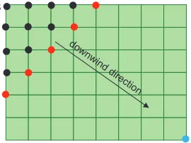
Fig. 3. Downwind wavefront propagation from source pointSto end pointEin parallel mode, so that at each iteration only the currently active nodes (red) propagate their weights to their neighbors simultaneously.
as shown in Fig 3. The algorithm starts from the source pointS, and at each iteration, a 1D arraycurrentArrayrecords the ID of theactive nodes. These are the nodes whose weights were changed at the last iteration and which will update their neighbors’ weights at the cur-rent iteration. Conceptually, this scheme is similar to the narrowband structure used by the fast marching method [32].
At each iteration, we use a ping-pong technique, with two 1D ar-rays,currentArrayandnextArray, being interleaved for consecutive iterations. currentArraystores the active nodes generated from the previous iteration and is used to launch the current iteration.nextArray stores the new active nodes generated at the current iteration and is used to launch the next iteration. Hence, whenever a node’s weight is changed, it will be recorded innextArrayat the current iteration, and will provoke the launch of a thread at the next iteration. To avoid a node being added to the same array multiple times during the parallel processing, a Boolean 3D array (mark) is used to record if a node has already been added to that array. All elements ofmarkare set to zero at the beginning of each iteration.
Active nodes behave like a wavefront, with information being prop-agated from the source nodeSto all other nodes in parallel. We clas-sify the grid points into three groups: discovered points, which were previously active but are not currently so (shown in black in Fig. 3); active points, whose weights were updated in the previous iteration (shown in red); andundiscovered points, which have not yet been vis-ited. At each iteration, we launch threads only foractive points– one thread for each active point. For a volume of a few million voxels, the number of active points (and thus also of the threads launched) is typi-cally in the order of thousands, which is much lower than the millions of threads required byb f p.
The pseudocode of im pis shown in Algorithm 3. In detail, we proceed as follows:
1. Given a source pointS, we setweight[S]to zero, appendSto currentArray, and set the array’s lengthcurrentLengthto 1. This array records all currently active nodes; these are the nodes that will propagate their weight information to their neighbors at the current iteration.
2. At each iteration, ifcurrentLength>0, we launch the paral-lel CUDA kernel on exactly currentLength GPU threads, one thread per elementCofcurrentArray. Each thread propagates the weight information fromCto its 26-neighbors, as in the brute force algorithmb f p. If an update of a neighborBis successful, we test ifBis already marked. If not, we mark it, append it to nextArray, and increment its length,nextLength. Usingmark avoids addingBtonextArraymore than once.
3. We swap currentArray and nextArray, and clear mark and nextLength, so that we can perform the next iteration. Steps 2 and 3 are repeated untilcurrentLength=0,i.e., until all nodes have been discovered and no node can be further updated.
Our improvedim palgorithm performs identically to theb f p al-gorithm, apart from skipping all of the unnecessary node evaluations,
Algorithm 3Improved parallel algorithm (im p)
1: blue// input:DFBcost,S,currentArray,currentLength,nextArray,nextLength,mark;
2: blue// output:weight;
3:
4: blue// Initialization:
5: SetMemory(mark,0); blue//clear all memory of arraymarkto zero
6: SetMemory(weight,MaxFloat); blue//set all memory toMaxFloat
7: weight[S] =0;
8: currentArray[0] =S;
9: currentLength=1;
10: nextLength=0;
11:
12: blue//iteration loop:
13: whilecurrentLength>0do
14: call the CUDA kernel ImprovedParallelIterationKernel(currentLength); blue//which launchescurrentLengthparallel threads, each running concurrently on a GPU core
15: Swap(currentArray,nextArray); blue//swap the memory address of the two arrays
16: currentLength=nextLength;
17: nextLength=0;
18: SetMemory(mark,0); blue//clear memory to zero
19: end while
20:
21: blue//the parallel CUDA kernel:
22: ImprovedParallelIterationKernel(threadID)
23: ifthreadID<currentLengththen
24: C=currentArray[threadID]; blue//concurrently retrieve an active nodeC
25: foreach neighborBofCdo// iterating on all 26 neighbors ofC
26: ifDFBcost[B]>0then
27: newWeight=weight[C] +DFBcost[B]; blue//potential new weight 28: oldWeight=atomicMin(weight[B],newWeight); blue//atomic operation
29: ifnewWeight<oldWeightthen
30: ifmark[B] ==0then
31: mark[B] =1; blue//mark it
32: oldIndex=atomicAdd(nextLength,1); blue//atomically add 1 to
nextLength
33: nextArray[oldIndex] =B; blue//appendBto the next iteration array
34: end if
35: end if
36: end if
37: end for
38: end if
so it produces exactly the same results as theb f sandb f palgorithms. We have confirmed this in practice by computing voxel-wise compar-isons of the results of the three algorithms.
The added value ofim pover the previous algorithms lies in three factors: (a) we do not need to maintain an expensive sorted queue; (b) instead of evaluating nodes one at a time, we evaluate multiple nodes in parallel on the GPU – a deterministic result is ensured by use of monotonically decreasing information propagation and by CUDA’s atomic operations; (c) at each iteration, only currently active nodes are evaluated, as opposed to the entire voxel set as in the brute force algorithms.
5.3 Centerline extraction by backtracing the MST
After the iterations in Algorithm 2 or 3 have terminated, the MST is available in the weight buffer. Having performed the compute-intensive calculations on the GPU, the remainder of the algorithm is performed on the CPU. We thus transferweightfrom the GPU mem-ory to the CPU memmem-ory and extract the centerline on the CPU by a simple backtracing which traverses the MST from the target end point Ealong the gradient direction of theweightfield until the source point Sis found.
In detail, at each stepiof the traversal, we test the 26-neighbors of the current nodeCi(initialized asC0=E), and choose the one with the minimum weight as the next current nodeCi+1. We repeat this process
until we find the source pointSas the last nodeCn−1. The desired
cen-terline is formed by the point sequence[C0,C1,C2,C3, ...,Cn−1]. The
number of steps of this process, equal to the length of the centerline,
is ofO(D)whereDis the diameter of the object, which is typically of the same order as the size of the space, i.e.,√3
Nfor a volume ofN voxels [27]. This step is very fast, and can be executed in real-time on the CPU.
Our approach could also be used to extract general 3D curve skele-tons including all branches. Since the MST connecting all of the inte-rior voxels has already been built, it is straightforward to find all other possible branches from the MST using the branch-finding method in-troduced in [40], and then merge them all into one topology.
6 RESULTS
The parallel algorithms presented above were implemented using CUDA 5 and tested on a PC computer with an Intel 3.5 GHz CPU and an NVIDIA GeForce GTX 690 graphics card. Although the GTX 690 has two GPUs, one is sufficient to handle all of our datasets, re-sulting in a usage of 2 GB video memory and 1536 CUDA cores. For examination and comparison, the centerlines extracted were displayed at a screen resolution of 1024×768 pixels.
As in previous serial approaches [40], our method can extract cen-terlines from either volume data (CT or MRI) or polygonal mesh mod-els, as long as a 3D DFB field (as input to our centerline algorithm) is pre-computed from the original object data, either from the segmented medical image slices or from the polygonal mesh.
The DFB pre-computation can be performed efficiently by recent GPU-based Euclidean distance transforms [11, 31] – for example, within a second for a volume of 5123 voxels on the hardware indi-cated above. The DFB pre-computation needs to be performed only once for a given model, after which the user can interactively specify the desired centerline start and end points and extract the actual cen-terlines. Since the focus of this paper is on centerline computation, we exclude the DFB pre-computation time from our runtime performance comparisons.
In our experiments, the user is presented with the input 3D surface, rendered semi-transparently. The user can next define the two end points by interactively clicking any two points in this rendered image. The selected points are shown as blue squares in all of the resulting images and videos. For each of the user’s clicks, the program will pick the 3D point on the frontmost surface layer of the object under the selected pixel, which is then used asSorE.
AfterSandEare defined, the centerline extraction algorithm is au-tomatically applied, and the resulting centerline points are displayed in real-time. Note that the two points selected must belong to a connected component of the object, otherwise an MST cannot be built connect-ing them. The interactive features of the algorithm can be seen in the accompanying videos. For comparison, the resulting images show the centerlines produced byserial,b f p, andim prendered in black, blue and red, respectively.
No parameters need to be set by the user at run-time, apart from the specification of the start and end points. For theb f palgorithm, threads are scheduled as 3D thread blocks on the GPU, with each block having 4×4×4 threads. For theim palgorithm, threads are scheduled as 1D thread blocks, with each block having 16 threads. We found that these are the optimized configurations and subsequently used them as presets in all our experiments.
6.1 Quality comparison
For all the shapes tested, the new algorithms managed to extract a visually correct and plausible centerline. In particular, we found that the centerlines respected the centeredness criterion well – no collision of the centerline with the input surface∂Ωwas found when directly examining the centerlines or using them as fly-through paths.
The key point is that the three queue-free methods (b f s,b f p,im p) are guaranteed to produce exactly the same results, and these results at worst show only very minor differences from those produced by the original queue-basedserialmethod. This proves that both parallel algorithms are robust, and their results are steady and deterministic. Because of this, the results ofb f sandb f pare not shown in Figure 6 to avoid redundancy.
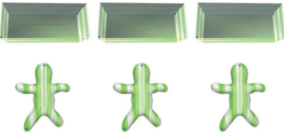
Figure 4 shows results for the blood vessel model at three differ-ent resolutions. It also shows that the higher the data resolution is, the smoother the centerline will be, though the computation time will be longer (see Table 1). In Figure 5, the three algorithms were tested on a cuboid and a doll model. Figures 4 and 5 demonstrate that the three algorithms produce identical centerlines for these simple-shaped models. These experiments were run multiple times, and all three al-gorithms always produced the same centerlines, as tested by a voxel-by-voxel comparison.
For other complex models, the voxel-by-voxel comparison indi-cated that there can be some differences between the centerlines pro-duced by theserial and parallel algorithms. However, these differ-ences are so small that they are not easy to notice, as can be seen in the examples in Figure 6.
The reason behind the differences is that the weight values are accu-mulated in our parallel algorithms, but not in theserialalgorithm, as explained in Section 4. Theserialalgorithm uses a pathlink for each voxel to label its predecessor. In contrast, the parallel algorithms use the gradient direction of the accumulated weight-field to find a voxel’s predecessor node.
As a desirable by-product of the weight accumulation, we note that the results produced by the parallel algorithm are smoother for com-plex models than those produced by theserialalgorithm. This is be-cause accumulating the weights acts as a low-pass filter of the result-ing centerline. This effect is especially obvious for thedinoSkeleton model in Figure 6, where the surface of the tail of the dinosaur ex-hibits high-frequency variations. These cause theserialalgorithm to produce a centerline with high-frequency noise, whereas our parallel algorithm filters such noise and hence produces a smoother centerline. This shows that our method is less sensitive to small-scale perturba-tions of the input surface than theserialalgorithm.
6.2 Performance comparison
We have performed extensive experiments on a wide range of datasets. The performance statistics corresponding to Figures 4, 5 and 6 are shown in Table 1. All algorithms were tested on the hardware men-tioned at the beginning of Sec. 6. Theserialcode was our implemen-tation based on the flowchart provided in [40].
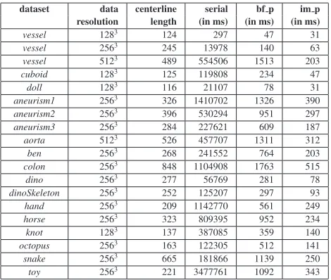
From Table 1, it is clear thatim pis up to 7 times faster thanb f p, which is itself significantly faster thanserial. On a broader front, if we compare our parallel centerline extraction (im p) with recent mesh and volume-based curve-skeleton algorithms [3, 20, 27, 35, 37], we observe thatim pis one to two orders of magnitude faster on similar hardware and for the same input datasets. As such, our algorithm presents con-crete added value in an interactive context, as in such situations post-processing the curve skeleton output of the latter algorithms would not be able to deliver interactive frame rates. Interestingly, our method is also faster than mesh-based curve-skeletonization algorithms [37], in-cluding carefully GPU-parallelized ones [20], which stand out for their high throughput.
6.2.1 Performance analysis
The improved parallel algorithmim pis much faster than any previ-ous algorithm but it does not sacrifice accuracy for speed. Its high per-formance is due to the parallel execution of many concurrent CUDA threads on many GPU cores.
[image:9.612.316.551.114.313.2]Our analysis showed that, as in all other MST-based centerline ex-traction algorithms, the bottleneck of ourim palgorithm lies in the MST computation stage, which accounts for more than 90% of the total time. The MST backtracking is very light and accounts for less than 10% of the time.
Table 1. Performance comparison over a range of datasets. The table shows the data resolution, the length of the extracted centerline (number of nodes along the centerline), and the extraction time (in milliseconds) of the algorithms serial, b f pandim p, respectively. The respective centerlines extracted are shown in Figures 4, 5 and 6.
dataset data centerline serial bf p im p resolution length (in ms) (in ms) (in ms)
vessel 1283 124 297 47 31
vessel 2563 245 13978 140 63
vessel 5123 489 554506 1513 203
cuboid 1283 125 119808 234 47
doll 1283 116 21107 78 31
aneurism1 2563 326 1410702 1326 390
aneurism2 2563 396 530294 951 297
aneurism3 2563 284 227621 609 187
aorta 5123 526 457707 1311 312
ben 2563 268 241552 764 203
colon 2563 848 1104908 1763 515
dino 2563 277 56769 281 78
dinoSkeleton 2563 252 125207 297 93
hand 2563 209 1142770 561 249
horse 2563 323 809395 952 234
knot 1283 137 387085 359 140
octopus 2563 163 122305 512 141
snake 2563 665 181866 1139 250
toy 2563 221 3477761 1092 343
In terms of complexity, theserialalgorithm requiresKiterations for an input shape withKvoxels, and at each iteration, it needs to sortM elements in the priority queue. Hence, its complexity isO(K×logM), as the sorting complexity isO(logM)at best. Here,Mis the number of active nodes currently in the queue, that is,Mis the length of the priority queue at each iteration. However,Mis not a fixed value over different iterations – it will increase rapidly as the iterations proceed because, at each iteration, as many as 26 neighbors of an active node will be inserted into the queue and only one node (the head) will be removed from it.
HenceM can become very large, which makes sorting the queue very time-consuming. As the sorting takes place after each of the fre-quent node insertions, this becomes the bottleneck of the serial algo-rithm. In our experiments, we found that the value ofMdepends upon the shape of the object: the fatter the object is, the more active nodes will accumulate in the queue from the previous iterations, so the larger the queue will become. For example, thecuboidmodel in Figure 5 is wide and this will cause a large number of voxels to be accumulated in the queue; as a result, for this model, the serial algorithm is 500 times slower than even the brute-force parallel algorithm, and thou-sands of times slower than theim palgorithm. This also explains why theserialalgorithm took 13 seconds for thevesselmodel but an hour for thetoymodel, even though both models have the same 2563 reso-lution. This is because the values ofKandMare much larger for the toy model than for the vessel model, even though the resolutionNof both models is the same.
The computational complexity of theb f palgorithm isO(N×I), whereIis the number of iterations, which is a bounded value because after information is propagated to reach all interior nodes the iteration procedure will stop. At each iteration, allNnodes of the dataset need to be evaluated regardless of whether they are active or not, however this is performed in a parallel mode by launchingNconcurrent CUDA threads. As a result it could still be hundreds of times faster than the serialalgorithm.
The complexity of im p is O(currentLength×I). It again per-forms in a parallel mode, but instead of evaluating all N nodes at each iteration, it evaluates only currentLength nodes by launching currentLengthconcurrent CUDA threads. Here,currentLengthis the number of the currently active nodes (recorded in currentArray) at each iteration – this can be thought of as equivalent to the length of the
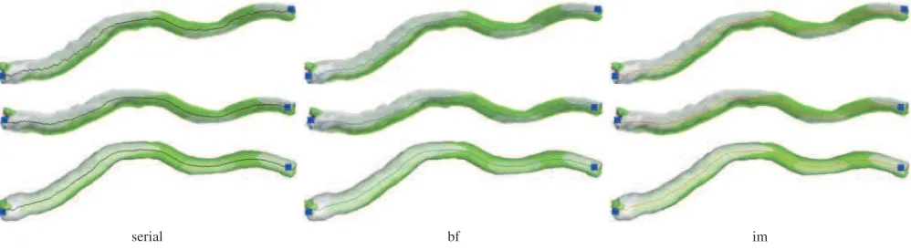
serial bf im
Fig. 4. Results produced by the three algorithms (left to right:serial,b f pandim p) for a blood vessel model (femoral artery) at three different data resolutions (top to bottom rows:1283,2563and5123, respectively). In each row, the three algorithms produce identical results; in each column,
the dataset with the higher resolution produces a smoother result. Please zoom in to see the details. The corresponding performance statistics for these images are shown in Table 1.
priority queue (the active set) in the serial algorithm. But the differ-ence here is that only the currently new “active” nodes at the current iteration need to be inserted intonextArray. Previously active nodes incurrentArraywill be inserted intonextArrayonly if they are again active (that is, their weight is again changed) at the current iteration. As a result, the active set remains much smaller during the ping-pong process than inserial.
Intuitively, the size of the active set inim p(i.e.,currentLength) at a certain iteration is the size (or area) of the wavefront patch shown in Fig. 3, which is a relatively smooth one-voxel-thick surface patch that propagates from the source point and is ‘cut’ by the object’s sur-face. At each iteration, one wavefront is replaced by another one-voxel-thick wavefront in the active set. IfI is the number of such wavefront patches during the propagation, then typicallyIis roughly of the same order as the diameter of the object i.e.,√3
Nfor a volume ofNvoxels).
In theserialalgorithm, the size of the active set,M, is more like a sub-volume or volumetric fraction of the object – it is much thicker than our wavefront patch. This is caused by node accumulation – at each iteration, only one node is removed from the queue but up to 26 nodes are inserted into it. As a result, many historically active nodes are accumulated in the queue as the iterations progress, and the size of the active set can become as large as a volumetric fraction of the object, i.e., of the same order asK. This explains why it performs much more slowly thanim p
In theory, theim palgorithm could also be implemented on a multi-core CPU, but the latest CPUs still have only very few multi-cores (up to 8 cores, generally). As, typically, thousands of nodes have to be evalu-ated concurrently at each iteration, 8 cores are far too few to provide a suitable level of parallelism compared to what is available on a modern GPU.
6.3 Comparison with latest curve-skeleton algorithms
Curve skeletons are different from centerlines, as we outlined in Sec-tion 1, and are not as suitable as centerlines for direct use as fly-through paths due to their branches and their inability to pass fly-through the predefined end points selected by the users. Nevertheless, for a greater insight into the performance of our method, we next compare the speed of our GPU centerline extraction with several state-of-the-art curve-skeleton algorithms.
Arcelliet al.[3] reported average times of 35 seconds for extracting the curve skeleton of 1283 resolution volumetric models, including similardinoandhorsemodels to those in Table 1, on a 3 GHz CPU. This implies that our method is hundreds of times faster (even more so since we used a higher resolution of 2563for these two models).
We have run the binary code provided by the authors of [27] on the machine used for Table 1, and the curve-skeleton extraction time of their algorithm for the horse dataset is 19.52 seconds, which is slower
than ourim pmethod by a factor of almost 100.
We also ran the binary code provided by the authors of [4], which is the most well known geometric approach for extracting curve skele-tons directly from mesh surfaces. The curve-skeleton extraction time for the same horse model was 960 seconds, which is much slower than our methods and the other voxel-based methods. However, this method has a much lower memory consumption, since it does not need to store the volumetric datasets.
The method of Jalbaet al.[20] uses GPU acceleration and requires, on a GTX 280 card, between 3 and 9 seconds (with an average of 4 seconds) to extract curve skeletons from models similar to the ones in Fig. 6,e.g.5.3 seconds forhorseand 3.8 seconds forhand. This com-pares to our 0.23 and 0.24 seconds, respectively, for the same models. Allowing for the fact that the GTX 690 GPU is 3 times faster than the GTX 280 GPU, our method remains 5 to 7 times faster, and it also has the advantage of a much simpler implementation.
As a final remark, we note that for applications such as fly-through path planning, which requires a single branchless centerline that passes through two user-defined end points, our algorithm is much more eco-nomical than these curve-skeleton methods. Even if such methods were to process the skeleton as efficiently asim p, time-consuming postprocessing would still have to be performed to remove undesired minor branches from the skeleton to produce a major trunk as the final fly-through path.
6.4 GPU Memory consumption
The main memory consumption of theim palgorithm lies in three 3D arrays. Besides the 3D texture ofDFBcostin float format, we also need
a float 3D arrayweightand a Boolean 3D arraymarkin byte format. So for a 5123dataset, e.g. the vessel and aorta in Table 1, the GPU memory consumption is 5123×(4+4+1)bytes,i.e.,128×9 MB = 1152 MB.
For larger datasets, such as 10243, the memory consumption could become a problem for a single GPU. To alleviate this, one could use half-precision floating-point format, which occupies 16 bits. This is commonly employed in GPU computing and has produced acceptable results for many applications. The various Boolean arrays can be fur-ther compressed to use one bit per voxel instead of 1 byte per voxel. Furthermore, recent GPUs, such as the NVIDIA GeForce Titan, have 6 GB GPU memory, which is sufficient to handle a 10243dataset at half-precision floating-point format. As such, we consider that our imple-mentation is suitable for use with normal real-world volume datasets without further modification. In the future, we will investigate using multi-GPUs to deal with even larger datasets.
6.5 Applications to virtual endoscopic simulation
naviga-Fig. 5. More identical results produced by the three algorithms (from left to right:serial,b f pandim p) for thecuboidanddollmodels, respectively. Please zoom in to see the details. The corresponding performance statistics for these images are shown in Table 1.
tion, etc., in virtual endoscopic simulation applications.
It can provide flexible real-time navigation paths based on user-specified end points within a 3D virtual model acquired from a con-tinuous sequence of 2D medical image slices scanned from the human colon, aiming to detect early-stage colon polyps. It can extract a cen-terline hundreds of times faster than the previous serial approach, in fact, so fast that the user will hardly notice any latency – in consid-erably less than a second in all of our experiments. This can be very helpful in assisting an interactive virtual endoscopic diagnostic pro-cess, as we show in the accompanying video, which uses the extracted centerline directly as the camera path (for theaneurism2 dataset). The video shows that the camera path is highly centered and smooth, and never collides with the object wall.
The extracted centerlines can also provide accurate measurements of the locations of abnormalities. For example, once a polyp is de-tected during a colon navigation, the physician immediately knows its location and the distances to the two end pointsSand E, which is useful for registration in surgery.
7 CONCLUSION
We have introduced a parallel algorithm, suited to modern GPU hard-ware, to extract centerlines automatically at interactive speed. Exper-iments have shown that the proposed algorithm is hundreds of times faster than the previous serial algorithm.
The proposed new algorithmim pis not only fast, but also has other desirable features, including precision, connectivity, simplicity, and computational efficiency.
The algorithm can produce a 26-connected highly centered singular path which is exactly 1-voxel thick, by construction. The centeredness of our centerline is derived from the DFB field. No ad hoc adjustments are needed to push the path back to the center.
Since our centerlines are extracted from the MST in the DFB field, they inherit the simplicity of the paths in a tree structure. In other words, the algorithm generates centerlines of 1-voxel width between the two end points (S and E), with no 2-D manifolds or 3-D self-intersections. This is important for automatic camera-path planning, as it avoids folding or self-intersection of the navigation path thus re-moving the possibility of “Y” junctions that can cause ambiguity and hesitation in the traversal.
The centerlines produced have the correct tendency to stay close to the local center of the object, due to the fact that the computation is based on an accurate DFB field with the exact Euclidean values. Another advantage is that the centerlines produced can be smoother than those of the serial algorithm due to the low-pass filtering effect of the new algorithm.
The algorithm is robust and deterministic, and is easy to understand, implement and maintain as its main concept is straightforward due to the precise and concise centerline definition.
REFERENCES
[1] L. Antiga. Patient-Specific Modeling of Geometry and Blood Flow in
Large Arteries. PhD thesis, Politecnico di Milano, Dipartimento di
Bioingegneria, Italy, 2002.
[2] L. Antiga. VMTK - the vascular modeling toolkit.
http://www.vmtk.org/index.html, 2012.
[3] C. Arcelli, G. Sanniti di Baja, and L. Serino. Distance-driven skeletoniza-tion in voxel images.IEEE TPAMI, 33(4):709–720, 2011.
[4] O. K.-C. Au, C.-L. Tai, H.-K. Chu, D. Cohen-Or, and T.-Y. Lee. Skele-ton extraction by mesh contraction. ACM TOG, 27(3):44:1–44:10, Aug. 2008.
[5] S. Aylward and E. Bullitt. Initialization, noise, singularities, and scale in height ridge traversal for tubular object centerline extraction. IEEE
Transactions on Medical Imaging, 21(2):61–75, Feb. 2002.
[6] X. Bai, L. Latecki, and W. yu Liu. Skeleton pruning by contour partition-ing with discrete curve evolution.IEEE TPAMI, 29(3):449–462, 2007. [7] I. Bitter, A. Kaufman, and M. Sato. Penalized-distance volumetric
skele-ton algorithm.IEEE TPAMI, 7(3):195–206, 2001.
[8] I. Bitter, M. Sato, M. Bender, K. McDonnell, A. Kaufman, and M. Wan. CEASAR: a smooth, accurate and robust centerline extraction algorithm.
InProc. IEEE Visualization, pages 45–52, 2000.
[9] A. Bleiweiss. GPU Accelerated Pathfinding. InProceedings of the 23rd
ACM SIGGRAPH/EG Symp. on Graphics Hardware, pages 65–74,
Sara-jevo, Bosnia-Herzegovina, 2008.
[10] H. Blum. A transformation for extracting new parameter of shape. In
Models for the Perception of Speech and Visual Form, MA: MIT Press,
1967.
[11] T.-T. Cao, K. Tang, A. Mohamed, and T.-S. Tan. Parallel banding algo-rithm to compute exact distance transform with the GPU. InProc. ACM
[image:11.612.57.544.68.302.2]SIGGRAPH Symp. on Interactive 3D Graphics and Games, pages 83–90, 2010.
[12] N. Cornea, D. Silver, and P. Min. Curve-skeleton properties, applications, and algorithms.IEEE TVCG, 13(3):530–548, May-June 2007. [13] L. Costa and R. Cesar. Shape analysis and classification: Theory and
practice, second edition. CRC Press, 2000.
[14] T. K. Dey and J. Sun. Defining and computing curve-skeletons with medial geodesic function. InProc. SGP, pages 143–152. Eurographics, 2006.
[15] Y. Ge, D. R. Stelts, and D. J. Vining. 3D skeleton for virtual colonoscopy.
InProc. Intl. Conf. on Visualization in Biomedical Computing, pages
449–454, London, UK, UK, 1996. Springer-Verlag.
[16] M. S. Hassouna and A. A. Farag. Robust centerline extraction framework using level sets. InProc. IEEE CVPR, pages 458–465, 2005.
[17] T. He and A. Kaufman. Collision detection for volumetric objects. In
Proc. IEEE Visualization, pages 27–34, 1997.
[18] W. H. Hesselink and J. B. T. M. Roerdink. Euclidean skeletons of digital image and volume data in linear time by the integer medial axis transform.
IEEE TPAMI, 30(12):2204–2217, 2008.
[19] H. Homann. Implementation of a 3D thinning algorithm. http://hdl.handle.net/1926/1292, Oct. 2007.
[20] A. C. Jalba, J. Kustra, and A. C. Telea. Surface and curve skeletonization of large 3D models on the GPU.IEEE TPAMI, 35(6):1495–1508, 2013. [21] J. Latombe.Robot Motion Planning. Kluwer, second edition, 1991. [22] J. Ma, S. Bae, and S. Choi. 3D medial axis point approximation using
nearest neighbors and the normal field. The Visual Computer, 28(1):7– 19, 2012.
[23] A. Meijster, J. B. T. M. Roerdink, and W. H. Hesselink. A general al-gorithm for computing distance transforms in linear time. In J. Goutsias, L. Vincent, and D. S. Bloomberg, editors,Mathematical Morphology and
its Applications to Image and Signal Processing, pages 331–340. Kluwer,
2000.
[24] K. Palagyi and A. Kuba. Directional 3D thinning using 8 subiterations. In G. Bertrand, M. Couprie, and L. Perroton, editors,Discrete Geometry
for Computer Imagery, volume 1568 ofLNCS, pages 325–336. Springer,
1999.
[25] G. Peyre and L. Cohen. Geodesic computations for fast and accurate surface remeshing and parameterization. InProgress in Nonlinear
Dif-ferential Equations and Their Applications, volume 63, pages 151–171.
Springer LNCS, 2005.www.ceremade.dauphine.fr/˜peyre. [26] C. Pudney. Distance-ordered homotopic thinning: A skeletonization
al-gorithm for 3D digital images.CVIU, 72(3):404–413, 1998.
[27] D. Reniers, J. van Wijk, and A. Telea. Computing multiscale curve and surface skeletons of genus 0 shapes using a global importance measure.
IEEE TVCG, 14(2):355–368, 2008.
[28] R. J. Sadleir and P. F. Whelan. Fast colon centreline calculation using optimised 3D topological thinning. Computerized Medical Imaging and
Graphics, 29(4):251–258, 2005.
[29] T. Saito and J.-I. Toriwaki. New algorithms for Euclidean distance trans-formation of ann-dimensional digitized picture with applications.Pattern
Recognition, 27(11):1551–1565, 1994.
[30] M. Schaap, C. Metz, T. van Walsum, A. van der Giessen, A. Weustinck, N. Mollet, C. Bauer, H. Bogunovic, C. Castro, X. Deng, E. Dikici, T. O’Donnell, M. Frenay, O. Friman, M. Hoyos, P. Kitslaar, A. Szym-czak, H. Tek, C. Wang, S. Warfield, S. Zambal, Y. Zhang, G. Krest-ing, and W. Niessen. Standardized evaluation methodology and reference database for evaluating coronary artery centerline extraction algorithms.
Med Image Anal, 13(5):701–714, 2009.
[31] J. Schneider, M. Kraus, and R. Westermann. GPU-based euclidean dis-tance transforms and their application to volume rendering. In A. Ran-chordas, J. Pereira, H. Aranjo, and J. Tavares, editors,Computer Vision,
Imaging and Computer Graphics. Theory and Applications, volume 68 of
Communications in Computer and Information Science, pages 215–228.
Springer-Verlag, 2010.
[32] J. Sethian. Level Set Methods and Fast Marching Methods, second edi-tion. Cambridge Univ. Press, 2002.
[33] E. Smistad. GPU-Based Airway Tree Segmentation and Centerline
Ex-traction for Image Guided Bronchoscopy. PhD thesis, Norwegian
Uni-versity of Science and Technology, 2012.
[34] E. Smistad, A. Elster, and F. Lindseth. Gpu accelerated segmentation and centerline extraction of tubular structures from medical images. Intl. J.
Computer Assisted Radiology and Surgery, pages 1–15, 2013.
[35] E. Smistad, A. C. Elster, and F. Lindseth. GPU-based airway tree
seg-mentation and centerline extraction for image guided bronchoscopy. In
Proc. Norsk Informatik Konferanse. Akademika Forlag, 2012.
[36] A. Sobiecki, H. Yasan, A. Jalba, and A. Telea. Qualitative compari-son of contraction-based curve skeletonization methods. In C. Hendriks, G. Borgefors, and R. Strand, editors,Mathematical Morphology and Its
Applications to Signal and Image Processing, volume 7883 ofLNCS,
pages 425–439. Springer-Verlag, 2013.
[37] A. Tagliasacchi, I. Alhashim, M. Olson, and H. Zhang. Mean curvature skeletons.CGF, 31(5):1735–1744, 2012.
[38] R. Van Uitert and R. Summers. Automatic correction of level set based subvoxel precise centerlines for virtual colonoscopy using the colon outer wall.IEEE Trans. Med. Imag., 26(8):1069–1078, 2007.
[39] M. Wan, F. Dachille, and A. Kaufman. Distance-field based skeletons for virtual navigation. InProc. IEEE Visualization, pages 239–560, 2001. [40] M. Wan, Z. Liang, Q. Ke, L. Hong, I. Bitter, and A. Kaufman. Automatic
centerline extraction for virtual colonoscopy. IEEE Trans. Med. Imag., 21(12):1450–1460, Dec. 2002.
[41] Y. Zhou and A. Toga. Efficient skeletonization of volumetric objects.
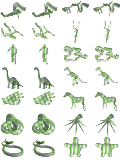
Fig. 6. Non-identical results produced byserial(left) andim p(right) algorithms. Please zoom in to see the details. From left to right, top to bottom, the datasets areaneurism1,aneurism2,aneurism3,aorta,ben,colon,dino,dinoSkeleton,hand,horse,knot,octopus,snake, andtoy, respectively.
12