The 4th International Conference on Computational Methods (ICCM2012), Gold Coast, Australia www.ICCM-2012.org
November 25-27, 2012, Gold Coast, Australia www.ICCM-2012.org
A new IRBFN scheme for the numerical simulation of interfacial flows
L. Mai-Cao1, T. Tran-Cong*2 1
Faculty of Geology & Petroleum Engineering, HCM University of Technology, Ho Chi Minh City, Vietnam 2
Comoutational Engineering and Science Research Centre (CESRC), Faculty of Engineering & Surveying, University of Southern Queensland, Toowoomba, Qld 4350, Australia
*Corresponding author: [email protected]
Abstract
This paper reports a new meshless scheme for the numerical simulation of interfacial flows in which the motion and deformation of the interface between two immiscible fluids are fully investigated. Unlike the passive transport problems studied in (L. Mai-Cao and T. Tran-Cong, 2008) where the influence of the moving interface on the surrounding fluid is ignored, the interfacial flows are studied in this paper with the surface tension taken into account. As a result, not only the position and shape of the moving interface but also the ambient flow variables (velocity field and pressure) change when the interface moves. In other words, a two-way interaction between the moving interface and the ambient flow is fully investigated. In this paper, the moving interface is captured by the level set method and the Navier-Stokes equations (with the surface tension embedded into the momentum equation) are used to model the ambient incompressible viscous flow in the meshless framework of the IRBFN method. A numerical simulation of two bubbles moving, stretching and merging in an incompressible viscous fluid is performed for verification purpose. Keywords: IRBFN, Meshless method, Level Set method, Interfacial flow, Front capturing
Introduction
Fluid flows with free moving interfaces between immiscible fluids can be classified as interfacial flows. Numerical methods for such flows are faced with several intrinsic difficulties. First, large differences in density and viscosity of the two fluids across the interface require appropriate treatments for the sharp interface resolution. Next, the moving interface might be subject to topological changes such as interface folding, breaking and merging. These phenomena must be numerically modelled with reliable algorithms. In addition, mass conservation is of primary concerns in numerical modelling of interfacial flows due to the existence of the fluid-fluid boundary, i.e. the moving interface itself.
the interface where the difference in stress tensors of the two fluids in the direction normal to the interface is equal to the surface tension force on the interface (Floryan, J.M. and Rasmussen, H., 1989). Simple implementations of such a interfacial boundary conditions in traditional methods have suffered from difficulties in modelling topologically complex interfaces. A numerical model for surface tension that alleviates these interface topology constraints was presented by (Brackbill, J.U. and Kothe, D.B. and Zemach, C., 1992). The proposed model, known as the continuum surface force (CSF) model interprets surface tension as a continuous, three-dimensional effect across an interface rather than as a boundary value condition on the interface. The advantage of this model is that the interface needs not to be explicitly described in order to apply the interfacial boundary condition. This well suits the interface capturing algorithm using the level set method which is used in this work.
Mathematical Formulation
Consider a domain Ω and its boundary containing two immiscible Newtonian fluids, both being incompressible. Let Ω1 be the region containing fluid 1 at time t. Similarly, let Ω2 be the region
containing fluid 2 and bounded by the fluid interface at time t. The governing equations describing the motion of the two fluids in their own regions are given by the Navier-Stokes equations,
1
1 1 1 p1 2 1 1 1 , x 1, t
v
v v D g (1)
2
2 2 2 p2 2 2 2 2 , x 2, t
v
v v D g (2)
with incompressibility constraints
1 0, 1
v x , v2 0, x2 (3)
where vi is the velocity field, i thedensity, g the gravity, pi the pressureand i is the viscosity. The rate of strain tensorDi is defined as
1
, 1, 2 2
T i i i i
D v v (4)
Assuming no mass transfer between the two fluids yields a continuity condition at the interface and the jump in normal stresses along the interface is balanced with the surface tension as follows
1 2,
v v x ,
21D122D2
n
p1p2
n x, (5) where is the curvature of the interface, the surface tension coefficient, and n is the unit normal vector along the fluidinterface pointing outwards relative to the fluid under consideration.
In this work, the continuum surface force (CSF) model is used to embed thesurface tension into the momentum equation rather than imposing the above equations on the moving interface (Brackbill, J.U. and Kothe, D.B. and Zemach, C., 1992).
Let the fluid interface be the zero level of the level set function such that { | ( , )x x t 0} where
12 ( , )
, 0
where d(x,t) represents the Euclidean distance from x to the interface. The unit normal on the interface, drawn from the interior into the exterior region, and the curvature of the interface can be expressed in terms of (x,t) as follows.
0 0 , = | | | |
n (7)
Let 1 1 2 2 v x v v x
be the fluid velocity continuous across the interface, since the interface moves with the fluid particles, the evolution of is then given by (Osher, S. and Fedkiw, R., 2003).
0 t
v (8) By defining the Heaviside function H() and the fluid properties
0 if <0 ( ) 1/ 2 if =0 1 if >0 H
(9), 2 1 2
2 1 2
( ) ( ) ( ), ( ) ( ) ( ), H H
(10)
together with the CSF model (Brackbill, J.U. and Kothe, D.B. and Zemach, C., 1992), one obtains the Navier-Stokes equations for two immiscible fluids known as the one-fluid continuum formulation (Chang, Y.C. and Hou, T.Y. and Merriman, B. and Osher, S., 1996) as follows.
1
2 ( ) ( ) ( ) ,
( ) p d
t
v
v v D n g (11)
0
v , (12) or in dimensionless form
1 1
12 ( ) ( ) ( ) ,
( ) p Re o
t B
v
v v D g (13)
where the Reynolds number (Re) and Bond number (Bo) are defined as follows.
3/2 2
1 1
1
(2 ) 4
Re R g ,Bo gR
(14)
The dimensionless density and viscosity in Equation (13) are defined as follows. ( ) (1 ) ( ), and ( )= +(1- ) ( ) H H
(15)
where 2 2
1 1
, =
are the density ratio and viscosity ratio, respectively.
Numerical Scheme
Step 0: Initialize the level set function (x,t=0) to be the signed distance to the interface as described in Equation (6).
For each time step tn, n=1,2,...
Step 1: Compute the interface normal, curvature, and the density and viscosity of the fluids, using Equations (7) and (15);
Step 2: Solve the one-fluid continuum Navier-Stokes equations using the IRBFN-based projection schemes (Mai Cao, L. and Tran-Cong, T., 2011) taking into account the interface dependence of density and viscosity as well as the surface tension;
Step 3: Advance the level set function from the previous step to the current one with the most updated velocity field by solving Equation (8) using the IRBFN-based level set schemes presented in (Mai-Cao, L. and Tran-Cong, T., 2008);
Step 4: Re-initialize the level set function to a signed distance function at the current time step and adjust the level set function by using the mass correction algorithm to ensure the mass conservation (Mai-Cao, L. and Tran-Cong, T., 2005, 2008);
Step 5: The interface as the zero contour of the level set function has now been advanced one time step. Go back to step 1 for further evolution of the moving interface until the predefined time is reached.
Numerical experiment and discussions
In this numerical experiment, a rectangular cavity is filled up with two immiscible fluids where the heavier one settles at the bottom and the lighter one at the top. Two bubbles, containing the same light fluid as in the top layer, are initially embedded in the heavier fluid at the bottom, one above the other. The bubbles are then released from rest and allowed to rise by buoyancy force. Four primary parameters are chosen as follows: Reynolds number Re=10; Bond number Bo=5; Density ratio =1/10; Viscosity ratio =1. It is noted that the density ratio indicates that the fluid inside the bubbles and in the top layer is ten times lighter than the heavier fluid. For this numerical simulation, the new numerical scheme presented in the previous section is used on a regular computational grid with 21 points in x-direction and 41 points in y-direction.
Figure 1. Numerical result at t=0.1 and t=0.2. Initially separated from the upper one, the lower bubble moves faster due to the wake formation below the upper one.
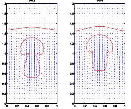
Figure 2. Numerical result at t=0.3 and t=0.4. The two bubbles merge together and continue to move
upwards.
Figure 3. The bubbles are about to reach the free surface at t=0.5 and t=0.6. The curvature of the surface shows the effect of the surface tension in keeping the kinematic equilibrium on the free surface.
Figure 4.Numerical results at t=0.7 and t=0.8. The bubbles finally reach and break through the interface. This also causes the bubbles to diffuse themselves into the surrounding fluid.
[image:5.595.305.521.110.290.2]Figure 5. The shape of the free surface after breaking and the velocity field at t=0.9 and t=1.0.
[image:5.595.306.524.554.744.2]When the bubbles get closer to the free surface at time t=0.5 and t=0.6, due to its surface tension, the free surface tends to prevent the upward motion remarkably. In their turn, the bubbles in keeping their trend to move upward make the free surface bend upwards more significantly. Figures 3 and 4 clearly show the effect of the surface tension in keeping the kinematic equilibrium on the free surface.
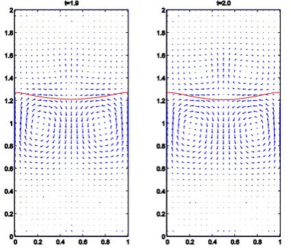
[image:6.595.59.276.256.445.2]In addition, the presence of the vorticities at t=1.3 and t=1.4 in Figure 7 indicatesthe effect of the surface tension along the free surface on the velocity field even when the bubbles completely diffuse into thesurrounding fluid. In later time, the gradual disappearance of the two upper vortices corresponds to the decrease in curvature of the free surface as can be seen in Figure 8.
Figure 7. Velocity field in the numerical simulation of two bubbles rising up in a buoyancy-driven flow at t=1.3 and t=1.4. The presence of the vorticities
[image:6.595.302.516.257.439.2]indicates the effect of the surface tension along the free surface on the velocity field even when the bubbles have completely diffused into the surrounding fluid.
Figure 8. Numerical simulation of two bubbles rising up in a buoyancy-driven flow at t=1.5 and t=1.6. The gradual disappearance of the two lower vortices (compared to Figure 7) corresponds to the decrease in curvature of the free surface.
Figure 9. Numerical simulation of two bubbles rising up in a buoyancy-driven flow at time t=1.7 and t=1.8. The free surface is on the way to reach a new
equilibrium.
[image:6.595.303.516.523.704.2] [image:6.595.59.268.523.703.2]Conclusions
A new meshless IRBFN scheme has been reported in this paper for the numerical simulation of interfacial flows in which the motion and deformation of the interface as well as the interaction between the moving interface and the surrounding fluid are fully captured. The new approach consists of (a) the flow modelling scheme based on the IRBFN projection scheme (Mai Cao, L. and Tran-Cong, T., 2011); (b) the interface modelling scheme based on the meshless level set scheme (Mai-Cao, L. and Tran-Cong, T., 2008); and (c) the flow-interface coupling model based on the CSF model proposed by (Brackbill, J.U. and Kothe, D.B. and Zemach, C., 1992). Those ``ingredients" are brought together in the meshless framework of the IRBFN method and used in this work as a new numerical approach to interfacial flow simulations.
The new approach has been applied to the numerical simulation of the interfacial flows of two immiscible viscous fluids. The numerical results show that the new numerical scheme is capable of capturing primary phenomena of flows such as the deformation and topological change of the moving interfaces as well as the interaction between the interface and the surrounding fluid. This feature is naturally available without any special treatments as normally seen in other methods.
References
Brackbill, J.U. and Kothe, D.B. and Zemach, C. (1992). A Continuum Method for Modeling Surface Tension. Journal
of Computational Physics, 100 , pp.335-354.
Chang, Y.C. and Hou, T.Y. and Merriman, B. and Osher, S. (1996). A Level Set Formulation of Eulerian Interface
Capturing Method for Incompressible Fluid Flows. Journal of Computational Physics, 124 ,pp. 449-464.
Floryan, J.M. and Rasmussen, H. (1989). Numerical Methods for Viscous Flows with Moving Boundary. Applied
Mechanics Reviews, 42 (12) , pp. 323-341.
Mai-Cao, L. and Tran-Cong, T. (2011). Meshless Numerical Schemes for Unsteady Navier-Stokes Equations. The 1st
International Symposium on Engineering Physics and Mechanics (ISEPM) October 25-26, . Ho Chi Minh City,
Vietnam.
Mai-Cao, L. and Tran-Cong, T. (2005). A meshless IRBFN-based method for transient problems. CMES: Computer
Modeling in Engineering and Science, 7 (2) , pp.149-171.
Mai-Cao, L. and Tran-Cong, T. (2008). A Meshless Approach to Capturing Moving Interfaces in Passive Transport
Problems. CMES:Computer Modeling in Engineering and Sciences, 31 (3) , pp. 157-188.
Osher, S. and Fedkiw, R. (2003). Level Set Methods and Dynamic Implicit Surfaces. New York: Springer.
Osher, S. and Sethian, J.A. (1988). Fronts Propagating with Curvature-Dependent Speed: Algorithms Based on
Hamilton-Jacobi Formulations. Journal of Computational Physics, 79 , pp. 12-49.
Sussman, M. and Smereka, P. (1997). Axisymmetric Free Boundary Problems. Journal of Fluid Mechanics, 341 , pp.