Developing a numerical model for the design of sheet pile walls

University of Southern Queensland

Faculty of Health, Engineering & Surveying

Developing a Numerical Model

for the Design of Sheet Pile Walls

A dissertation submitted by

Chane Brits

in fulfilment of the requirements of

ENG4111 and ENG4112 Research Project

towards the degree of

Abstract

This project involves the investigation, development and validation of cantilevered and anchored sheet pile wall models. The effect of sheet pile construction penetrating a sandy soil are investigated by analysing numerical outputs such as the wall deformation, ground settlement and maximum bending moment. The numerical analysis is completed using an industrially known computer software program: Fast Lagrangian Analysis of Continua (FLAC).

The quality of the FLAC models used to obtain the numerical solutions was validated for accuracy against available analytical solutions. The aims of this project were to gain sufficient knowledge on sheet pile wall design methods, better known as the limit equilibrium methods; develop an automatic Excel spreadsheet as a design tool for solving any sheet pile wall design problem; and be able to easily validate the accuracy of the obtained numerical solutions by comparing the numerical and analytical solutions.

The main focus of the investigation was to develop new cantilever and anchored sheet pile wall models for a specific geotechnical problem of a sheet pile penetrating a sandy soil in the presence of a water table. This was done by validating the numerical models and undertaking parametric studies varying specific parameters to investigate thoroughly the behaviour of the sheet pile wall system.

University of Southern Queensland

Faculty of Health, Engineering and Sciences

ENG4111/ENG4112 Research Project

Limitations of Use

The Council of the University of Southern Queensland, its Faculty of Health, Engineering & Sciences and the staff of the University of Southern Queensland, do not accept any responsibility for the truth, accuracy or completeness of material contained within or associated with this dissertation.

Persons using all or any part of this material do so at their own risk, and not at the risk of the Council of the University of Southern Queensland, its Faculty of Health, Engineering & Sciences or the staff of the University of Southern Queensland.

University of Southern Queensland

Faculty of Health, Engineering and Sciences

ENG4111/ENG4112 Research Project

Certification of Dissertation

I certify that the ideas, designs and experimental work, results, analysis and conclusions set out in this dissertation are entirely of my own effort, except where otherwise indicated and acknowledged.

I further certify that the work is original and has not been previously submitted for assessment in any other course or institution, except where specifically stated.

Chane Brits

StudentNumber:0061007950

Signature _____________________________

Acknowledgements

IwouldliketotakethisopportunitytogivemyfullandsincerethankstoDrJim Shiau for his continued guidance, enthusiasm and support throughout the duration of this project. His experience and guidance on the subject has been extremely valuable and has led to the possibility of achieving set goals to an extraordinary standard. I would also like to thank my family for their constant support, encouragement and patience throughout the past four years of my continuous studies. Finally, special thanks to my fellow engineering friends Anthony Vadalma and Alejandro Aldana for all their positive feedback and motivation during this year.

With appreciation

Table of Contents

List of Figures ... viii

List of Tables ... x

Nomenclature ... xi

Chapter 1: Introduction ... 1

1.1 Background ... 1

1.2 Aims and Objectives ... 2

1.3 Overview of Chapters ... 3

1.4 Summary ... 5

Chapter 2: LiteratureReview ... 6

2.1 Introduction ... 6

2.2 BackgroundInformation ... 7

2.3 Classical Design Methods ... 14

2.4 Numerical Analysis and Dissertations ... 26

2.5 Numerical Modelling Methods ... 29

Chapter 3: Developing a Design Tool for Sheet Piles Walls ... 32

3.1 Introduction ... 32

3.2 The Analytical Methods ... 33

3.3 Design Procedure for Cantilever Sheet Pile Wall ... 34

3.4 Cantilever Sheet Pile Problem Description ... 38

3.5 Development of Excel Spread Sheet for the Cantilever Pile Problem ... 39

3.6 Design Procedure for Anchor Walls ... 45

3.7 Anchored Sheet Pile Problem Description... 47

3.8 Development of Excel Spread Sheet for Anchor Wall Problem ... 48

3.9 Comparison between Cantilever and Anchored Pile Outputs ... 52

3.10 Conclusion ... 53

Chapter 4: FLAC Overview ... 55

4.1 Introduction ... 55

4.2 Major FLAC Features ... 56

4.4 Chapter Summary ... 59

Chapter 5: Numerical Analysis of Cantilever Sheet Pile Walls ... 60

5.1 Introduction ... 60

5.2 Background Information ... 60

5.3 Problem Description ... 62

5.4 Analysis using FLAC ... 62

Chapter 6: Numerical Analysis of Anchored Sheet Pile Walls ... 79

6.1 Introduction ... 79

6.2 Background Information ... 79

6.3 Problem Description ... 80

6.4 Analysis using FLAC ... 80

Chapter 7: Conclusions ... 92

7.1 Spread Sheet Development for Sheet Pile Wall Design ... 92

7.2 Cantilever Sheet Pile Wall ... 92

7.3 Anchored Sheet Pile Wall ... 93

7.4 Future Work ... 94

7.5 Achievement of Objectives ... 95

List of References ... 97

Appendices ... 101

Appendix A: Project Specification ... 102

Appendix B: Cantilever Sheet Pile Wall-Limit State Method Calculations ... 104

List of Figures

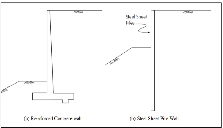
Figure 1-1: Retaining walls: (a) rigid wall, (b) flexible wall (Ramadan 2013) ... 7

Figure1-2:Cantilever Sheet Pile (Hauraki Pilling LTD) ... 11

Figure1-3:Macalloy Anchored Sheet Pile (Iceland, 2002) ... 12

Figure 1-4: Failure modes for anchored sheet pile walls (Caltrans 2004) ... 13

Figure 1-5: Failure modes for cantilevered sheet pile walls (Leila & Behzad 2011) .. 14

Figure 2-1: Full method (Padfield & Mair 1984) ... 15

Figure 2-2: Simplified method (Padfield & Mair 1984) ... 16

Figure 2-3: Rectilinear Earth Pressure Distribution (Bowles 1988) ... 17

Figure 2-4: Case studies by Day (1999) ... 18

Figure 2-5: Point of zero net earth pressure, presented by Day (1999) ... 19

Figure 2-6: Cantilever sheet pile penetrating sand (Das 1990) ... 20

Figure 2-7: Nature of variation of deflection and moment for anchored sheet piles: (a) free earth support method; (b) fixed earth support method (Das 1990) ... 21

Figure 2-8: Fixed Earth Support Method (Torrabadella 2013) ... 22

Figure 2-9: Free Earth Support Method (Torrabadella 2013) ... 23

Figure 2-10: (a) Coulomb wedge analysis, (b) Rankine ‘state of stress’ analysis (Keystone Retaining Wall Systems 2003) ... 24

Figure 2-11: Blum’s equivalent beam for anchored sheet pile wall design (Torrabadella 2013) ... 25

Figure 3-1: Displacement of Sheet Pile Wall: (a) Cantilever (b) Anchored (Yandzio 1998) ... 33

Figure 3-2: (a) Cantilever Pile Penetrating a Sandy Soil, (b) Active and Passive Pressure Distribution (Das 1990) ... 34

Figure 3-3: Cantilever Sheet Pile Problem Definition (Das 2007) ... 39

Figure 3-4: Hydrostatic equilibrium of fluid motion (Szolga 2010) ... 43

Figure 3-5: System of forces and moments (Szolga 2010) ... 44

Figure 3-6: Visual Diagrammatic Output Figures for a cantilever sheet pile ... 45

Figure 3-7: Anchored sheet pile penetrating a sandy soil (Das 1990) ... 46

Figure 3-8: Anchored sheet pile problem definition (Das 2007) ... 48

Figure 5-1: (a) Cantilever Pile Penetrating a Sandy Soil, (b) Active and Passive

Pressure Distribution (Das 1990) ... 60

Figure 5-2: Cantilever Sheet Pile Penetrating Sand: (a) Net Pressure Variation Diagram; (b) Moment Variation (Das 2007) ... 61

Figure 5-3: Problem to be Investigated ... 62

Figure 5-4: Assumed Course Mesh Grid ... 63

Figure 5-5: Column Removed for Sheet Pile Construction ... 65

Figure 5-6: Constructed Sheet Pile Wall Model ... 65

Figure 5-7: An Interface Represented by sides a, and b, connected by shear (ks) and normal (kn) stiffness springs (FLAC 2D online manual 2009) ... 66

Figure 5-8: FLAC Model Containing Course Mesh ... 67

Figure 5-9: (a) Grid, (b) Failure Surface for initially assumed Model ... 68

Figure 5-10: (a) Grid, (b) Failure Surface for Fine Mesh Model with Horizontal Increase ... 69

Figure 5-11: (a) Maximum Bending Moment, (b) Maximum x-Displacement ... 70

Figure 5-12: Plasticity Indicators for the Fine Mesh Model ... 71

Figure 5-13: Visual Comparison of Maximum Bending Moment ... 72

Figure 6-1: Problem to be investigated ... 80

Figure 6-2: Anchor Sheet Pile Wall Model ... 81

Figure 6-3: Node-to-node Anchors (Ramadan Amer 2013) ... 82

Figure 6-4: Visual Comparison of Maximum Anchor Tie Rod Force ... 83

Figure 6-5: Visual Comparison of Maximum Bending Moment ... 84

Figure 6-6: Failure Surface Plots; for (a) Cantilever Pile, (b) Anchored Pile ... 86

List of Tables

Table 3-1: Analytical Results for Cantilever Pile ... 38

Table 3-2: User Input Parameters ... 39

Table 3-3: Designer Selection for Kp ... 41

Table 3-4: Automatic Analysis of Analytical Equations ... 41

Table 3-5: Effect of Kp Selection on Sheet Pile Wall Length ... 42

Table 3-6: Important Theoretical Output Solutions ... 42

Table 3-7: Analytical Results for Anchored Pile ... 47

Table 3-8: User input data ... 49

Table 3-9: Automatic analysis of Analytical Equations ... 49

Table 3-10: Effect of Kp Selection on Sheet Pile Wall Length ... 49

Table 3-11: Important Output Solutions ... 50

Table 3-12: Comparison between Cantilever and Anchored Sheet Pile Wall ... 52

Table 3-13: Comparison between Cantilever and Anchored Sheet Pile Wall ... 53

Table 4-1: Grid Generation ... 58

Table 4-2: Soil Properties ... 58

Table 4-3: Pile Element Properties (ArcelorMittal 2013; Das 2007) ... 58

Table 4-4: Rod Anchor Properties (Ischebeck; FLAC 2D online manual 2009)... 58

Table 4-5: Solving Analysis ... 58

Table 4-6: Output Variables ... 59

Table 5-1: Comparison of Maximum Bending Moment ... 73

Table 5-2: Validation of FLAC Model ... 73

Table 5-3: Convergence Study of Varying Mesh Fineness ... 74

Table 5-4: Parametric Study of Soil Friction Angle ... 75

Table 5-5: Parametric Study of Ground Water Table ... 77

Table 6-1: Comparison of Maximum Bending Moment ... 85

Nomenclature

The principalsymbols used arepresented in thefollowing list.Locallyused notation andmodifications,suchasbyadditionofasubscriptorsuperscript,andasymbol that hasdifferentmeaningsindifferentcontextsaredefinedwhereused.

Ka Rankine’s Active Pressure Coefficient

K_p Rankine’s Passive Pressure Coefficient 𝜙 Un-drained internal friction angle of the soil ∅′ Drained internal soil friction angle

𝜎′ Pressure at a particular depth 𝛾 ′ _{Effective Soil unit weight}

𝛾 Soil unit weight 𝐿 Sheet Pile Length

𝛾_𝑠𝑎𝑡 Saturated unit weight of the soil 𝛾_𝑤 Unit weight of water

𝐷 Penetration depth of sheet pile

𝑃 Total active pressure behind sheet pile wall 𝑧 Depth below the ground surface

𝑧̅ Point of zero shear force below the ground surface 𝐴 Constant (in Chapter 3 section 3.5.3)

𝐹𝑂𝑆 Factor of safety 𝑐 ′ _{Drained soil cohesion}

𝑀_𝑚𝑎𝑥 Maximum bending moment exerted on sheet pile wall 𝐹 Anchor force

𝐷𝑡ℎ𝑒𝑜𝑟𝑒𝑡𝑖𝑐𝑎𝑙 Theoretical penetration depth of the sheet pile wall

𝐷_{𝑎𝑐𝑡𝑢𝑎𝑙} Actual penetration depth of the sheet pile wall 𝐴 Area (in Chapter 3 section 3.5.5)

𝑛 Number of elements

Chapter 1:

Introduction

This project investigates the suitability of modelling various geotechnical sheet pile wall problems using anexplicitfinitedifferenceprogram,FastLagrangianAnalysisof Continua (FLAC). This project encompasses research into available classical theories, current techniques of analysis and the creation of computer models. This research discusses the geotechnical problems analysed and presents the results of an investigation. The geotechnical problems to be investigated are:

 Cantilever Sheet Pile Wall Penetrating a Sandy Soil

 Anchored Sheet Pile Wall Penetrating a Sandy Soil.

1.1

Background

Geotechnical Stability

Ground stability must be assured prior to consideration of other foundation-related items. Foundation problems involve the support of natural soil. Stability problems often occur when building over soft, low strength soil. Problems with foundation stability can be prevented by initial recognition of the problem and appropriate design.

The design of all structures demands ultimate and serviceability limit state requirements to be satisfactory. Failure under ultimate limit state occurs when ‘a collapse mechanism takes place in the ground or in some parts of the structure’ (Lancellotta 1995). The failure mechanism can be divided into strength and stability components.

Choice of Models

The parametric study that will be conducted within this dissertation is a thorough study that aims to evaluate the effect of changing certain parameters on the behaviour of the pile-wall system. The parameters that will be investigated are:

 mesh fineness

 soil strength

 water table effect

 installation of anchor systems.

The anchored sheet pile wall model represents the possibility of decreasing the effect of the lateral earth pressures developed on the sheet pile wall. This problem was investigated to analyse the application of an anchor tie rod force on the behaviour of the sheet pile wall. Knowledge of these effects will aid in future studies within the area, as it is of upmost importance for a designer to analyse the sheet pile wall deformation for serviceability purposes and the bending moment analyses for structural design purposes. Due to its nature, FLAC has the potential to decrease the solution time and increase the accuracy of the results. The outcome will be a greater understanding of effective sheet pile wall design in the engineering industry.

Computational Analysis

Numerous methods have been developed to solve geotechnical stability problems by hand calculations; however, modern graphical software tools have made it possible to gain a much better understanding of the inner numerical details of soil-wall system behaviour. Comparing the numerical solutions to the analytical solutions, it is clear that more accurate solutions are now available by using modern computer software. However, to obtain useful results from a computer program, it is necessary to have an experienced user.

1.2

Aims and Objectives

evaluate the accuracy of FLAC and obtain more information and knowledge of the system. This will lead to more effective sheet pile wall design in the engineering industry.

The identification of appropriate milestones is an important part of reaching the major objectives within a given timeframe. The sequence of the tasks is briefly described below:

 Research background information on the application of numerical analysis for geotechnical design.

 Create a spread sheet in Excel that will automatically solve for any sheet pile wall design. Aim for this spread sheet to be useable in the engineering industry.

 Gain sufficient knowledge of the software program FLAC, to enable the writing of a script code using FLAC’s inner built-in coding language, FISH. This will make it possible to create an anchored sheet pile wall model in FLAC.

 Undertake parametric studies in FLAC by means of varying specific parameters to determine the effect of the net pressure, shear forces and bending moments applied on the sheet pile wall.

 Compare the results obtained from the analytical methods with the results gathered from the numerical applied analysis to verify the numerical methods.

1.3

Overview of Chapters

This chapter overview gives a brief introduction to the task, methodology and the computer program to be utilised. Following this, each problem is investigated separately, including validation and advanced parametric studies to analyse the behaviour of the sheet pile wall. The dissertation concludes with an overall summary and an outline of possible future work.

Chapter 1: Introduction

Chapter 2: Literature Review

This chapter presents a literature review of all the past studies for the design of cantilevered and anchored sheet pile wall problems. Included within the literature review are current available analytical methods for the design of sheet pile walls, as well as findings and results from past dissertational FLAC modelling of sheet pile walls. The previous work is used to determine why additional research is necessary and the scope of the research required.

Chapter 3: Developing Tools for Sheet Pile Wall Design

In this chapter, the methodology for designing sheet pile walls is introduced. Indicated in this chapter is the development of design tools such as an automated spread sheet that can automatically solve any sheet pile wall problem, solving tedious analytical equations within seconds by simply inputting known data specified by the user. The generated design tools are then used as part of the validation process of the numerical models.

Chapter 4: FLAC Overview

This chapter presents a short introduction to the FLAC software package, as well as an overview of the FLAC script that was generated to model the geotechnical problem. The methodology used for specifying the inputs required the development of a numerical model that leads to the validation of the models and specific outputs obtained from FLAC.

Chapter 5: FLAC Analysis of Cantilever Sheet Pile Wall

this chapter, advanced modelling by means of undertaking a parametric study has been presented to illustrate the overall soil-pile system behaviour.

Chapter 6: FLAC Analysis of Anchored Sheet Pile Wall

Presented in this chapter is the creation of a cantilever sheet pile wall model for the specific geotechnical sheet pile wall problem. This chapter presents the validation of the numerical model, as well as advanced modelling of anchorage sheet pile wall systems, to investigate specific parameters that have a ‘real life’ effect in the engineering industry.

Chapter 7: Conclusions and Future Work Recommendations

This chapter presents the overall findings presented within Chapters 3–6. This chapter presents a summary of the conclusion of the dissertation. Recommendations for further work are discussed to ensure that this work is clearly defined.

1.4

Summary

Chapter 2:

Literature

Review

2.1

Introduction

There are several sheet pile walls design methods dating back to the first half of the twentieth century. These original proposals have been continuously and may currently be being reviewed (Torrabadella 2013). Analytical methods include ‘limit stage design methods’ or ‘classical methods’ (King 1995). For establishing equilibrium of the horizontal forces and moments developed along the wall and to define the failure state point along the sheet pile and the embedment depth below the dredge line for either cantilever or anchored sheet pile walls by means of undertaking geotechnical design, calculations are required regardless of the method adopted.

The estimation of the limit equilibrium method depends on the limiting earth pressure coefficients from plastic theories. The earth pressure forces on the wall are also calculated with these plastic theory values. During the limit equilibrium condition, the equilibrium equations are used to deduce the driven depth of the sheet pile wall. A factor of safety is applied by an increase in sheet pile depth to limit the movement of the wall and take into account any possible errors in the soil parameters and analysis.

The second approach, the finite element technique, first proposed by Morgenstern and Eisentein (1970), often makes use of the finite element technique to solve the stiffness equations. Satisfactory knowledge of the stress-strain behaviours of the soil and its parameters is necessary, as this indicates the behaviour of the soil-structure system.

Equilibrium for an anchored sheet pile wall with only a single row of anchors can be achieved without taking into consideration the passive reaction at the bottom of the back of the sheet pile wall. However, the design method used can change depending on whether this reaction force is considered. When comparing the cantilevered and anchored sheet pile walls, the main advantage found from the anchored sheet pile wall is its ability to reduce the embedment depth of the sheet pile, thus increasing the excavation depth, which has a profitable effect on the structure (Das 1990). It is important to note that due to the anchor provided, the excavation depth can be increased, but the structure behaves like a cantilever sheet pile only until the anchor is placed (Torrabadella 2013).

2.2

Background

Information

Sheet pile walls consist of driven, vibrated or pushed interlocking pile segments embedded into soils to resist horizontal pressures. The sheet pile walls are constructed by driving the sheet piles into a slope or excavation. They are considered most cost-effective where retention of higher earth pressures of soft soils is required. Sheet piles have a significant advantage in that they can be driven to depths below the excavation bottom and so provide a control to heaving in soft clays or piping in saturated sand.

Sheet piles can function as temporary or permanent structures and are most often used in excavation projects. Temporary sheet piling structures are used to control or exclude earth or water and allow the continuation of permanent work. Permanent sheet piling is commonly used as a retaining structure, and at times as part of the structure of underground buildings (Paikowsky & Tan 2005).

When sheet pile walls are constructed, important design parameters are introduced that are often difficult to evaluate, making the design process complex and protracted. The generation of an automatic design tool in Excel to solve any sheet pile wall problem would help to overcome these design difficulties and time issues; not only by leading to easier evaluation, but also by making it possible to obtain results quickly for undertaking the validation process.

Numerical modelling has evolved over the years. Research has found that these numerical methods for the design of sheet pile walls are very useful and can be used to obtain information that is unavailable when using analytical methods for the design of sheet pile walls (Smith 2006; Bilgin 2010); that is, the wall deformation, ground settlement and possible surface failures. This research uses FLAC to develop its numerical model. FLAC is a popular industrially known design tool, used to solve geotechnical problems.

Sheet Pile Wall Materials

enduring structures are constructed of steel or concrete. Concrete is capable of providing a long service life under normal conditions, but has relatively high initial costs when compared to steel sheet piling. Concrete piling is also more difficult to install than steel piling. Long-term field observations indicate that steel sheet piling provides a long service life when properly designed (Ramadan Amer 2013).

The steel sheet pile alternative is the most popular due to its strength, ease of handling and construction. Steel sheet piles are available in various cross-section shapes. They can have problems with corrosion that can be prevented by coating. They can be used above or below water provided the required protection is applied (Bowles 1988).

Their advantages are:

 resistant to high driving stresses

 relatively lightweight

 reusable

 long service life

 easy to increase length by welding

 joints are less likely to deform

 can produce a watertight wall.

Other materials such as vinyl, polyvinyl chloride and fiberglass are also available. These pilings have very low structural capacities and function in tieback situations. When compared to other materials, only short lengths of pile are available. The designer for each sheet pile application when using one of the above-mentioned materials must carefully evaluate the properties of the specific material obtained from the manufacturer (Paikowsky & Tan 2005).

Construction of Sheet Pile Walls

The construction of sheet pile walls may involve either excavation of soils in front or backfilling of soils behind the wall; that is, fill construction or cut construction. Fill wall construction refers to a wall system in which the wall is constructed from the base of the wall up to the top: also called ‘bottom-up’ construction. Cut wall construction refers to a wall system in which the wall is constructed from the top of the wall down to the base, concurrent with excavation operations: known as ‘top down’ construction (Zhou 2006). These construction procedures generate different loading conditions in the soil and thus different wall behaviour should be expected (Das 1990).

Sheet pile walls are widely used in excavation support systems, cofferdams and cut-off walls under dams, slope stabilisation, waterfront structures and floodwalls. Sheet pile walls used to provide lateral earth support could be either cantilever or anchored depending on the wall height. Recently, land owners have been seeking to maximise the usage of their land by designing basements up to their land boundaries, with little regard for the subsoil and site condition restraints. The result is that various deep excavations are carried out in close proximity to existing buildings and infrastructures, increasing the importance in design of considering the safety of neighbouring structures (Kasim 2011).

Cantilever Sheet Pile Walls

capacity of the piles for stability (Figure 1-2). Therefore, it should not be used where the foundation material may be removed during wall service life (Caltrans 2004).

Figure1-2:Cantilever Sheet Pile (Hauraki Pilling LTD)

Anchored Sheet Pile Walls

Anchored sheet pile walls are required when the wall height exceeds 6 m or when the lateral wall deflection is limited for design consideration (Leila & Behzad 2011). Anchoring the sheet pile wall requires less penetration depth and also less moment to the sheet pile because it will drive additional support by the passive pressure on the front of the wall and the anchor tie rod. Anchored sheet pile walls are typically constructed in cut situations, and may be used for fill situations with special design considerations to protect the anchor from construction damage from fill placement or fill settlement (Geotechnical design procedure for flexible wall systems 2007).

Horizontal struts need to be used when the width of excavation is small and when their usage does not affect the construction of permanent elements; inclined rakers are used for wide excavation. According to Gulhati and Datta (2008), grouted tiebacks and dead-man anchors are used when there is available underground space beyond the excavated area. This space should be free from the foundations and the underground utilities of adjacent structures.

Figure1-3:Macalloy Anchored Sheet Pile (Iceland, 2002)

Sheet Pile Wall Failure Mechanisms

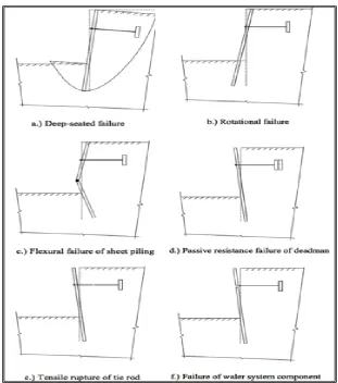
When analysed as retaining structures, several failure modes for a sheet pile system must be considered in the design process (US Army Corps of Engineers, 1996). These failures include deep-seated failure, rotational failure due to pile penetration inadequacy, overstressing of the sheet pile and anchorage component failure. An investigation of the load capacity of piles subjected to combined loading was performed, as second-order bending effects reduce the lateral load capacity of the wall when piles are exposed to combined axial and lateral loads (Greimann 1987).

prevented by adequate wall penetration into the soil or by implementing an anchorage system.

The other failures that may occur in retaining wall systems are sheet pile overstressing, passive anchorage failure, tie rod failure and wale system failure (Figure 2-4). In the case of pile overstressing due to both lateral and axial loads, a plastic hinge leading to failure will develop.

When the anchor moves laterally within the soil due to the force exerted on it, a passive anchorage failure will occur. The tie rod may fail if the required tensile capacity is not adequate, and the wale system may undergo a bearing failure if the loads are not evenly distributed (Evans 2010).

Figure 1-5: Failure modes for cantilevered sheet pile walls (Leila & Behzad 2011)

2.3

Classical Design Methods

There are several design methods that make different assumptions and hence make different simplifications of the net pressure distribution exerted along the sheet pile wall. In this section, the classical design methods of sheet pile walls are discussed. The current limit state design method most commonly used in the United Kingdom (UK) is the UK method, as described by Padfield and Mair (1984). In the United States (US), the USA method, or gradual method, as described by Bowles (1996), is the most commonly used limit state design method. Suggesting a rectilinear pressure distribution leads to the simplifying of the net pressure distribution along the sheet pile wall. An analytical limit equilibrium approach has been suggested by King (1995), involving an empirically determined parameter. The net pressure distribution has been examined using finite element analysis by Day (1999).

Chapter 3. In addition, in Section 2.4, discussion is presented of some dissertations on numerical sheet pile wall design (Smith 2006; Ramadan 2013; Torrabadella 2013).

Padfield and Mair (1984) Design of Retaining Walls in Stiff Clays

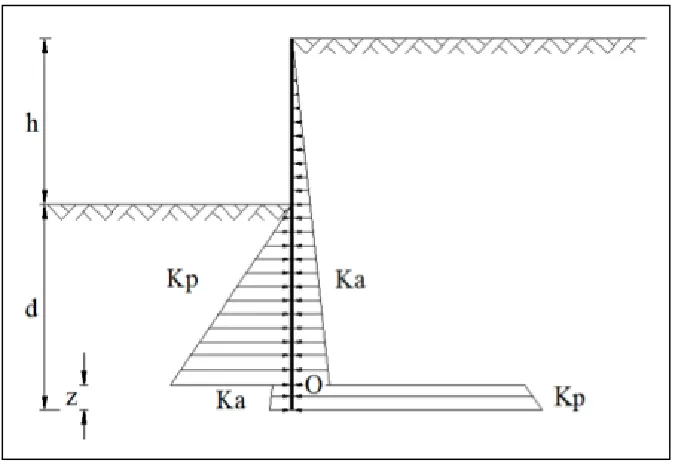
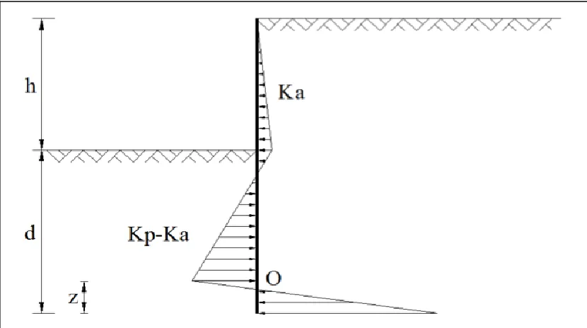
The full UK method gets its name in contrast to the simplified method, described below. In the full method, the active limit state is assumed to be reached in the back of the wall above the rotation point, and the passive limit state is assumed to be reached in front of the wall between the dredge line and the rotation point. Supposedly, an overturn in the normal pressure direction is to be produced at the rotation point, below which the full passive pressure is moved behind the wall and the active to the front. This causes a sudden jump in the earth pressure, which is needed to prescribe moment equilibrium.

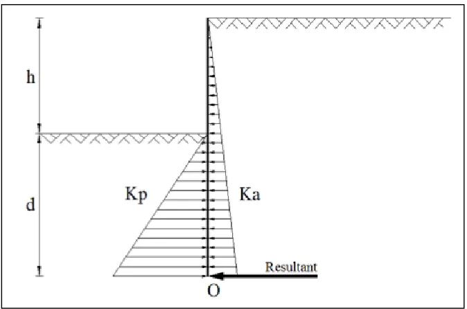
Due to the complexity of the full method, a simplification was recommended by Padfield and Mair (1984). As shown in Figure 2-2, the earth pressure below the rotation point can be replaced by an equivalent concentrated force acting on point O, represented as the resultant force. The value for the depth d has been found to be considerably lower than compared to the value calculated by the full method. Thus, the simplified method is slightly more conservative than the full method, although it leads to appreciably similar results.

Bowles (1988) Foundation Analysis and Design

A rectilinear net earth pressure distribution was proposed by Bowles (1988) in which the active earth pressure in the back of the wall above the dredge line and passive earth pressure in front of the wall immediately below the dredge line were fully mobilised even before failure. The design depth of penetration was calculated by finding the z in Figure 2-3, corresponding to the maximum net earth pressure in front of the wall, satisfying both equilibrium of horizontal forces and moments about the bottom of the wall.

Figure 2-3: Rectilinear Earth Pressure Distribution (Bowles 1988)

Day (1999) Net Pressure Analysis of Cantilever Sheet Pile Walls

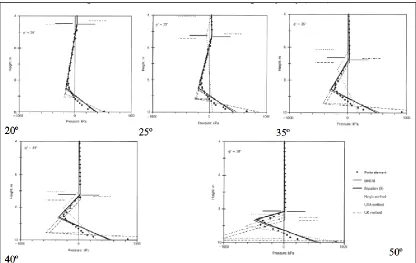
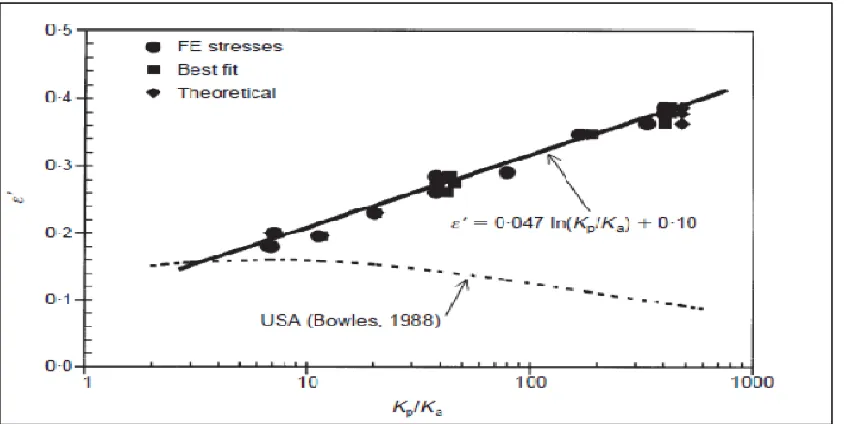
Day (1999) presented a finite element study in which the net earth pressure over the sheet pile wall was examined. In the finite element study conducted by Day (1999), five case studies were considered, consisting of wall heights of 10 m and soil friction angles ranging between 20 and 50 degrees with variable excavation depths. The results indicated that a dependent relationship exists between the point of zero net pressure and the ratio between the active and passive pressure distributions (Figure 2-4).

Day proposed an equation to define the point of zero pressure (Figure 2-5). This equation proposed a linear relation between the position of the point of zero pressure and the ratio of Kp to Ka. The proposal by King (1995) that 𝜀′= 0.35 is generally conservative.

Figure 2-5: Point of zero net earth pressure, presented by Day (1999)

The rectilinear net pressure distribution and pressure coefficients predicted by Caquote and Kerisel are more accurate than the existing design methods commonly used in the UK and US. According to Day (1999), the predictions for both the critical retained height and the bending moment distribution using the empirical equations agree excellently when compared to the finite element numerical results for cantilever sheet pile walls. The finite element results are in fact in better agreement with Caquote and Kerisel’s results than the existing design analytical methods.

Das (1990) Principles of Foundation Engineering

The wall rotates about a point O (Figure 2-6 [a]). The hydrostatic pressures on either side of the sheet pile wall are assumed to cancel each other out; thus, only considering the effective lateral soil pressure below the dredge line to act on the sheet pile was assumed. In zone A, the lateral pressure is just the active pressure from the land side; however, in zone B, there will be active pressure from the land side as well as passive pressure from the water side due to the yielding occurrence of the wall. The condition in zone C is reversed, which is below the point O. The actual net pressure distribution on the wall is shown in Figure 2-6 (b), and a simplified version is illustrated in Figure 2-6 (c).

Figure 2-6: Cantilever sheet pile penetrating sand (Das 1990)

The two basic methods of designing anchored sheet pile walls are (a) the free earth support method and (b) the fixed earth support method. According to Das (1990), the free earth support method involves a minimum penetration depth to be obtained and the absence of a pivot point for the static system (Figure 2-7).

Fixed Earth Support Method for Anchored Piles

In the fixed earth support method, the sheet pile is embedded deeply in comparison with the height above the dredge level in such a way as to ensure that the passive pressure in front of the wall is no longer fully mobilised. An overturn in the normal earth pressure is achieved by means of the increasing embedment depth. The earth pressure distribution results is similar to that achieved for the cantilever sheet pile wall (Figure 2-8). The wall behaves as if partially built-in and being subjected to bending moments (United States Steel 1975).

Figure 2-8: Fixed Earth Support Method (Torrabadella 2013)

Free Earth Support Method for Anchored Pile

enough to withstand such pressures (Shanmugam 2004; Das 1990). The entire depth of embedment mobilises the shear strength of the soil (Figure 2-9).

Proceeding then by means of summing the moments with respect to the point of applied anchor force and equating the expression to zero, the minimum embedment depth is calculated to provide equilibrium.

Figure 2-9: Free Earth Support Method (Torrabadella 2013)

The theory and assumptions made by Das (1990) for the development of the lateral earth pressures exerted on the sheet pile wall are based on Rankine theory. There are two commonly accepted methods for calculating simple earth pressure (Keystone Retaining Wall Systems 2003): Coulomb and Rankine theory. The Coulomb theory was developed in 1776, while the Rankine theory was developed in 1857. These theories, which remain the basis for present-day earth pressures calculation, are based on the fundamental assumptions that the retained soil is:

 cohesionless

 homogenous

 isotropic

 semi-finite

The active earth pressure calculation requires that the wall structure rotates or yields sufficiently to engage the entire shear strength of the soils involved to create the active earth pressure state. The amount of movement highly depends on the soil that is involved.

Both theories use identical parameters; however, Coulomb wedge theory calculates less earth pressure than Rankine theory (Figure 2-10). This indicates that the results obtained from the Rankine theory will be more conservative. Das (1990) made use of these conservative methods for the design of sheet pile walls.

Figure 2-10: (a) Coulomb wedge analysis, (b) Rankine ‘state of stress’ analysis (Keystone Retaining Wall Systems 2003)

Blum’s (1931) Equivalent Beam Method Theory for Anchored Piles

The moments are taken around the point in line with the anchor force for the upper part of the beam to find the force Rb; in the lower beam, moments are taken at the bottom to

find the embedment depth (Figure 2-11). The embedment depth must be increased to ensure that the reaction Rc can be engaged (Azizi 2000; Bowles 1996; Tsinker 1997).

Figure 2-11: Blum’s equivalent beam for anchored sheet pile wall design (Torrabadella 2013)

Conclusion of Classical Method Design

2.4

Numerical Analysis and Dissertations

Smith (2006), Development of Numerical Models for Geotechnical Design

Smith (2006) investigated a cantilever sheet pile wall penetrating sand in the absence of a water table using the finite difference method software, FLAC. The numerical results obtained from the numerical model developed in FLAC were then compared to the analytical solutions and the advantages and disadvantages were discussed. The depth of embedment was then varied to identify the effect exerted on the sheet pile wall by analysing the bending moment, wall deflection and ground settlement. Smith’s (2006) investigation demonstrated that FLAC produced similar results to the limit equilibrium methods. The outputs obtained were also found to be more accurate when compared to the limit equilibrium method solutions. Smith (2006) suggested the possible future work of undertaking numerical parametric studies using the cantilevered sheet pile wall model to develop an anchored sheet pile wall model. Performing parametric studies was also deemed valuable for the advanced analysis of the behaviour of the sheet pile walls.

Bilgin (2010), Numerical Studies of Anchored Sheet Pile Wall Behaviour Constructed in Cut and Fill Conditions

deformations. These findings indicate that there are limitations to be considered when using the limit equilibrium methods, and that more information can be obtained by undertaking numerical analysis (Bilgin 2010).

Bilgin (2012), Lateral Earth Pressure Coefficient for Anchored Piles

According to Bilgin (2012), the design of anchored sheet pile walls established by the conventional methods is based on the lateral force and moment equilibrium of active and passive earth pressure and anchor forces. Bilgin (2012) carried out a parametric study using both conventional and numerical methods to investigate the behaviour of a single-level anchored sheet pile wall. The effect on the wall lateral earth pressures, wall moments and anchor forces was investigated. The results obtained indicated that the free earth support method over-estimates the bending moments, whereas the anchor forces were underestimated. Interestingly, new lateral earth pressure coefficients that took the stress concentration around the anchor level into account were used in the design, which led to more realistic earth pressure distributions acting on the wall, as well as more accurate anchor sheet pile wall designs.

Ramadan (2013), Effect of Wall Penetration Depth on the Behaviour of Sheet Pile Walls

Torrabadella (2013), Numerical Analysis of Cantilever and Anchored Sheet Pile Walls at Failure and Comparison with Classical Methods

Torrabadella (2013) analysed the influence of the initial stress state condition on the horizontal displacement of sheet pile walls. It was found that for K0 values between 0.7

and 0.9, minimum movement was registered at the top of the pile; however, the initial stress state also depended on the soil friction angle. Depending on the initial stress state, the wall movement was found potentially to change up to 40%. The influence of the construction procedure also had a critical effect on the wall movement. For anchored piles, it was found that when the anchors were pre-stressed, movement was absorbed, limiting wall strains. In contrast to cantilever sheet pile walls, the maximum horizontal displacement was found at a particular depth and not at the ground surface. A direct effect between the anchor force and horizontal wall displacement was found. Torrabadella (2013) also found that the limit equilibrium methods corresponded well with the numerical methods for both cantilever and anchored sheet pile walls.

Zhai (2009), Comparison Study for the Seismic Evaluation of Anchored Sheet Pile Walls

2.5

Numerical Modelling Methods

Most engineering problems involve complex physical phenomena (Chaskalovic 2008). To gain a good understanding of these phenomena, engineers normally make simplified assumptions that allow the formulation of mathematical models (Pastor & Tamagnini 2004; Wood 2003).

Numerical analysis has evolved over the past few decades (Chaskalovic 2008), followed by prompt advances and improvements in modern computer technology (Rao 2005; Zienkiewicz, Taylor & Zhu 2013; Desai and Christian 1977). This will lead to the ability to undertake procedures, algorithms and other numerical techniques capable of solving ever more complex engineering problems. However, it is important for an engineer to know that with these numerical methods certain limitations, uncertainties and approximations need to be considered (Wood 2003). This leads to more computationally based studies being carried out in the geotechnical engineering industry. It is important that the results obtained from the numerical methods are validated against conventional or analytical methods (Pande & Pietruszczak 2004).

Industrially Commonly Known Numerical Analysis

The most common numerical techniques used currently in the geotechnical engineering industry are the finite difference method (FLAC) and the finite element method (PLAXIS). Finite difference methods were almost exclusively used in obtaining numerical solutions for geotechnical problems prior to the establishment of the finite element methods. The finite element method is considered one of the most important developments in civil engineering of the twentieth century (Papadrakakis 2001).

Background of FLAC Software

elements or zones that can be adjusted by the user. This explicit, Lagrangian calculation scheme and the mix-discretisation zoning technique used in FLAC ensure the highly accurate modelling of flow and plastic collapse. Large 2D calculations can be made without the need for massive memory requirements due to no matrixes being formed.

FLAC was originally developed for geotechnical and mining engineers. This software offers a wide range of capabilities, including for solving complex problems in mechanics. The FLAC software has special built-in functions that make it unique. The application range of FLAC is extensive because it is equipped with 11 built-in constitutive models, five optional facilities and several kinds of structure elements as well as a built-in coding language, FISH (Shen 2012).

Other element structures present in FLAC include beam, anchor, pile and shell structures. These elements are used to create more realistic models of geotechnical engineering problems in the software. It will be useful to design an anchored sheet pile wall model in FLAC. The build-in coding language (FISH) can also be used to define new functions and variables to meet user demands.

FLAC Software Advantages and Disadvantages

The FLAC software, used here to develop a numerical model for the design of sheet pile walls, has several advantages over other methods (FLAC 2D online manual 2009):

 The mix-discretisation zoning method is more accurate than the reduced integration method generally used to simulate the plastic flow of materials.

 The explicit methods used decrease the time needed to solve non-linear equations.

 The full dynamic equation of motion is used, making the software more suitable to simulate problems involving vibration, failure and large deformations.

 The element numbering is done in row and column formatting.

 FLAC depends on the ratio of maximum and minimum natural periods of the system for the convergence velocity.

Chapter 3:

Developing a Design Tool for Sheet Piles Walls

3.1

Introduction

Nowadays, the engineering profession is discovering and using the computational powers of computer spread sheets in practice. They are used in bid preparation, budgeting, control, engineering design computation and many other areas. However, the computational power of the computer spread sheet is only the beginning of what can be accomplished. The success of geotechnical works relies on the proper planning, analysis and design of sheet pile walls. The analytical methods normally consist of many equations and may take a long time to solve by hand. This chapter gives an overview of how the tedious equations obtained by the analytical methods for the design of sheet pile walls are used to develop design tools in an Excel spread sheet that can automatically solve any sheet pile wall design problem in a matter of seconds.

3.2

The Analytical Methods

A sheet pile wall is an alternative to using a gravity retaining wall to support retained material. It consists of vertical structural elements implanted at adequate depth into the soil beneath the specific granular material to be retained (Day 1999). Several sheet pile walls design methods exist, dating back to the first half of the twentieth century. These original proposals have been continuously and may currently be being reviewed. To define the embedment depth below the dredge line for cantilever and anchored sheet pile walls, geotechnical design calculations using analytical methods are used for establishing equilibrium of the horizontal forces and moments developed along the wall (Figure 3-1).

3.3

Design Procedure for Cantilever Sheet Pile Wall

Cantilever sheet pile walls are usually recommended for walls of moderate height (6 m or less, measured above the dredge line). In such walls, the sheet piles act as a wide cantilever beam above the dredge line. The net lateral pressure distribution on a cantilever sheet pile wall can be explained by the basic principles of Das (1990), with the aid of Figure 3-2 (a).

It has been assumed that the straight planes represent the ground and failure surfaces and that the resultant force acting on the backfill slope is acting in a parallel direction. Both active and passive pressure zones will develop on either side of the sheet pile wall, as indicated in Figure 3-2 (b).

Due to this development of both active and passive pressures, it is necessary to determine the Rankine’s active and passive pressure coefficients:

Ka= tan2(45 − ϕ/2 ) (3-1)

Kp= tan2(45 + ϕ/2) (3-2)

Where

𝜙 - Angle of friction of sand

It is important to note that after conducting a geotechnical survey, the designer will know certain input parameters. This is important information, as it gives knowledge about the type of soil, the friction angle of the soil, the length above the dredge line and the soil cohesion.

Knowing this input data, the active pressure on the right side of the sheet pile wall can be determined:

σ1′ = γL1Ka (3-3)

σ2′ = (γL1+ γ′L1) K_a (3-4)

Where

𝛾 - Unit weight of the soil above the water table

𝛾 ′ - Effective unit weight of the soil = 𝛾_𝑠𝑎𝑡− 𝛾_𝑤

At the level of the dredge line, the hydrostatic pressure on both sides of the wall is equal in magnitude and hence cancels out. As indicated in Figure 3-2 (a), the net pressure will be equal to zero at the point E. Hence, using the ratio given as 1 vertical to γ′_(K

p− Ka)

in the horizontal, the unknown length L3 can be determined:

L3 = σ₂; γ′_(K

p− Ka) (3-5)

P = 0.5 σ₁;L₁+ σ₁;L₂+ 0.5(σ;₂− σ₁;)L₂+ 0.5σ₂;L₃ (3-6) Summing the moments of all the pressure forces exerted on the wall about point E and dividing by the total pressure force P will provide the distance 𝑧̅ from E to the force P.

𝑧̅=

⌈ ⌈ ⌈ ⌈ ⌈ ⌈

0.5σ₁;L1 ∗(𝐿₃1+ 𝐿2+ 𝐿3)+

σ₁;L2∗(𝐿3+𝐿₂2)+

0.5(σ₂; − σ₁;)L₂∗(𝐿₃+𝐿2

3)+

0.5σ₂;L3∗𝐿₃3 ⌉⌉ ⌉ ⌉ ⌉ ⌉

𝑃

⁄ (3-7)

Thus, the only unknown is the length of L4, which is determined by deriving four

equations containing the unknown length L4 by:

 the formation of an equation for p₃ using the given ratio of 1 vertical to γ′_(K p−

K_a) in the horizontal (3-8)

 determining the net pressure p4 at the bottom of the sheet pile by subtracting

the total active pressure from the total passive pressure (3-9)

 summing the moments about the point B at the bottom of the sheet pile (3-10)

 deriving an equation for the length L5, which forms a part of the unknown length

L4 (3-11).

σ₃; = 𝛾′L₄(K_p− K_a) (3-8)

σ₄; = σ₅; + 𝛾′L₄(K_p− K_a) (3-9) 𝑃(𝐿4+ 𝑧̅) − (0.5𝐿4σ3

;_{) (}𝐿4

3) + 0.5𝐿5(σ3 ;

+ σ₄;)(𝐿5

3) (3-10)

𝐿₅ = σ3;L4− 2P

σ₃; + σ₄;

⁄ (3-11)

These four equations are then rearranged to determine L4, solving an equation to the

fourth power:

Where A1, A2, A3 and A4 are given by Das (1990):

𝐴₁= σ5;

𝛾′_(𝐾

𝑝−𝐾𝑎) (3-13)

𝐴2= _𝛾′_(𝐾8𝑃

𝑝−𝐾𝑎) (3-14)

𝐴3=

6𝑃[2𝑧̅𝛾′_(𝐾

𝑝−𝐾𝑎)+𝑝5]

𝛾′ 2 _(𝐾 𝑝−𝐾𝑎)2

(3-15)

𝐴4=

𝑃[6𝑧̅𝑝₅+4𝑃] 𝛾′ 2 _(𝐾

𝑝−𝐾𝑎)2

(3-16)

Where p₅ is the passive pressure applied above point E.

The decline in active pressure immediately above point E due to the large passive pressure being exerted on the left side of the sheet pile wall is given by:

p₅= (γL1+ γ′L2)𝐾𝑝+ 𝛾′𝐿3(K_p− 𝐾𝑎) (3-17)

Knowing the length L4, the sheet pile penetrating depth is simply:

𝐷𝑡ℎ𝑒𝑜𝑟𝑒𝑡𝑖𝑐𝑎𝑙= 𝐿3+ 𝐿4 (3-18)

It is important for designers to note that a certain factor of safety (FOS) has to be satisfied to avoid any possibility of soil-system failure. It is at the discretion of the designer to apply a FOS to the calculated sheet pile penetrating depth or to decrease the overestimated Rankine’s passive pressure coefficient. According to Das (1990), it is recommended to apply a FOS of between 1.5 and 2.

As already mentioned, it is important to determine the maximum bending moment distributed on the sheet pile wall for design purposes. Thus, the sheet pile is analysed as a normal beam to find the point of zero shear force:

Z′ =√_(K 2P

Knowing the maximum bending moment will occur at this point, the moments about the point of zero shear force are summed:

Mmax = P(𝑧̅ + 𝑍′) − [0.5𝛾′_𝑍′2_(K

p− Ka)]( 𝑍′

3) (3-20)

Table 3-1: Analytical Results for Cantilever Pile

Parameters Results

Length (m) L4 5.95

Theoretical Penetration Depth (m) Dt 6.51

Factor of Safety FOS 1.40

Actual Penetration Depth (m) Da 9.12

Total Wall Length (m) Ltot 18.12

Maximum Bending Moment (kN.m) Mmax 741

Obtaining these solutions using the tedious analytical equations to be solved by hand takes a long time and is prone to human error. Thus, being able to solve many different sheet pile wall problems in a matter of minutes would be useful for the engineering industry.

3.4

Cantilever Sheet Pile Problem Description

The following example is solved analytically using the procedure detailed in Das (1990). The example is then solved in an Excel spread sheet developed by this study so that the relevance of developing design tools for cantilevered sheet pile walls can be understood.

For the example in Figure 3-3, the cantilever sheet pile wall is penetrating a sandy soil and therefore has zero cohesion. The friction angle 𝜙 and unit weight 𝛾 of the sandy soil were obtained from Das (1990). The solutions obtained for this example using the analytical limit equilibrium methods are tabulated in Section 3.5.

Figure 3-3: Cantilever Sheet Pile Problem Definition (Das 2007)

3.5

Development of Excel Spread Sheet for the Cantilever Pile

Problem

The aim in developing the Excel spread sheet was that it could automatically solve complex derived analytical equations by means of a user inputting known data (Table 3-2) into the spreadsheet.

Table 3-2: User Input Parameters

Parameters above the dredge line Parameters below the dredge line

Depth (m) L1 3 Depth (m) L2 6

Unit weight of soil (𝑘𝑁_𝑚3) 𝛾𝑑𝑟𝑦 18.85 Unit weight of soil (

𝑘𝑁

𝑚3) 𝛾𝑠𝑎𝑡 20.33

Cohesion of soil (𝑘𝑁

𝑚2) c1 0 Cohesion of soil (

𝑘𝑁

𝑚2) c2 0

Angle of Internal Friction (Degrees) ∅ 40 Angle of Internal Friction

(Degrees)

∅ 40 Effective Unit weight of soil (_𝑚𝑘𝑁3) 𝛾′ 0 Effective Unit weight of soil (

𝑘𝑁

𝑚3) 𝛾′ 10.52

𝐿1= 3 𝑚

𝛾 = 18.85𝑘𝑁

𝑚3

𝑐′_{= 0}

∅′_{= 40°}

D

𝐿₁ = 6 𝑚 𝛾_𝑠𝑎𝑡 = 20.33𝑘𝑁

𝑚3

𝑐′ _{= 0}

∅′ _{= 40°}

Sheet Pile Wall

Known Geotechnical Input Data

The input data give an outline of the design problem, such that the total depth above the dredge line is the sum of length 1 and length 2, giving 9 m. Normally, cantilever sheet pile walls are used for heights of less than 6 m (Das 1990), indicating that this sheet pile wall is very long. The unit weight of the dry soil at a depth of 3 m from the ground surface is 18.8 𝑘𝑁⁄_𝑚3 and the unit weight of the saturated soil below the water table is 20.33𝑘𝑁⁄_𝑚3. The effective unit weight of the soil is found by subtracting the unit weight of water (9.81𝑘𝑁⁄_𝑚3) from the saturated unit weight of the soil, which

gives 10.52𝑘𝑁⁄_𝑚3. The soil type is classified as a sandy type soil. Therefore, the cohesion of the soil above and below the water table is equal to zero. The internal friction angle of the sandy type soil is 40 degrees.

Designer Selection of Factor of Safety

As mentioned, when using the analytical methods, it is recommended to apply a FOS either at the beginning of the problem or at a later stage by increasing the theoretical penetrating depth of the sheet pile. This decision influences the final solutions obtained for the total length of the sheet pile and the point on the structure at which zero shear force occurs; hence, the maximum bending moment will also be affected.

The designer using the Excel spread sheet is given the option of inputting the FOS value required and selecting one of two options, as follows:

(1)Kp (Rankine’s passive pressure coefficient) is used when the FOS should be applied to the calculated theoretical penetration depth of the sheet pile. Then the non-factorised passive pressure coefficient will be used (Kp).

Kp = 3.25 from (3-2)

Kp design = Kp/FOS (3-21) = 2.5

Since the FOS was selected as 1.4 (Table 3-3), it was assumed that the output results and solutions for using both cases of Rankine’s passive pressure coefficient would be equal. However, after analysing the solutions, this was found not to be the case.

Table 3-3: Designer Selection for Kp

FOS Kp Kp design

1.4 4.6 3.29

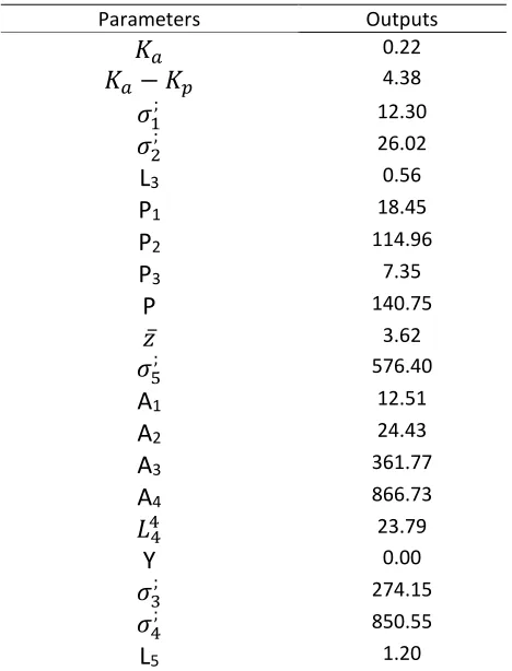
Automatic Analytical Analysis

A separate section of automatic analysis was next derived in Excel to solve all the analytical equations. This is identified in the Excel spread sheet under automatic analysis:

Table 3-4: Automatic Analysis of Analytical Equations

Parameters Outputs

𝐾_𝑎 0.22

𝐾𝑎− 𝐾𝑝 4.38

𝜎₁; 12.30

𝜎₂; 26.02

L3 0.56

P1 18.45

P2 114.96

P3 7.35

P 140.75

𝑧̅ 3.62

𝜎₅; 576.40

A1 12.51

A2 24.43

A3 361.77

A4 866.73

𝐿4₄ 23.79

Y 0.00

𝜎₃; 274.15

𝜎₄; 850.55

If a FOS is applied to Rankine’s passive pressure coefficient before the automatic analysis commences, to reduce the passive pressure coefficient, the theoretical depth obtained when using a factored passive coefficient is found to be 6.06% smaller than an un-factored passive pressure coefficient (Table 3-5).

Table 3-5: Effect of Kp Selection on Sheet Pile Wall Length

Parameters Kp design Kp Percentage difference (%)

Total theoretical length 16.51 15.51 6.06

Total actual length 16.51 18.12 8.88

Point of zero shear force 2.95 2.47 16.27

The application for reducing the passive pressure coefficient compared to applying a FOS to the theoretical penetration depth will lead to an 8.88% decrease for the actual factored penetrating sheet pile wall length.

The point of zero shear force on the sheet pile wall will decrease by 16.27% when applying a FOS during the automatic analysis. This affects theoretical penetration depth.

An indirect relationship was found between the actual wall penetration depth and the point of zero shear force on the pile. If the actual wall penetration depth increases, the point of zero shear force decreases.

Important Output Values

The important output values such as length L4, theoretical depth Dt, actual depth Da and

maximum bending moment Mmax were next obtained (Table 3-6).

Table 3-6: Important Theoretical Output Solutions

Parameters Kp design Kp Percentage difference (%)

Theoretical Penetration Depth 7.51 6.51 13.31

Actual Penetration Depth 7.51 9.12 17.65

It can be seen that when a FOS is applied to the passive pressure coefficient compared to applying the FOS to the theoretical pile penetration depth, the theoretical penetration depth of the sheet pile increases by 13.31% with the reduction of Rankine’s passive pressure coefficient. This causes the pile penetration depth to remain constant for both theoretical and actual wall penetration depths.

Applying a FOS to the theoretical penetration depth will lead to an increase of 17.65% to the actual penetration depth. The increase of the actual penetration depth reduces the maximum bending moment by 5.84% for the un-factored passive pressure coefficient compared to the factored passive pressure coefficient. This formulates an indirect relation between the theoretical and actual penetration depths, as well as between the actual penetration depth and the maximum bending moment obtained.

Graphical Visual Representation

As the analytical methods and calculations do not indicate the outputs graphically, a simple table has been developed to give graphical visual outputs for the deformation, shear force and bending moments distributed along the sheet pile wall.

The pressure diagram in Figure 3-4 was established by knowing the pressure at certain points on the sheet pile wall as calculated using the analytical equations.

Figure 3-4: Hydrostatic equilibrium of fluid motion (Szolga 2010)

Where P is the pressure (𝒌𝑵

𝒎𝟐

⁄ )

F is the force (𝒌𝑵)

By interpolating between the known depths, it was possible to find the pressures corresponding to the increasing depths. The shear force at known depths were calculated for a 1m-wide strip using equation (3-22) and similarly interpolating between two values and multiplying by a half to find the specific shear force at a particular depth. The maximum bending moment was calculated using equation (3-23) for specific depths and interpolating between values for increasing sheet pile depth.

Net ShearForce = pressure ∗ (length ∗ width) (3-22) Net Bending Moment = force ∗ distance (3-23) From the hydrostatic equilibrium of fluid motion, the force applied on an object is a vector, while the pressure is a scalar. For a force produced by pressure, it is necessary to consider a surface with a certain area and direction.

In statics, moments are effects (of a force) that cause rotation. When commuting equilibrium, it is necessary to calculate the moment for every force that has been generated on the object. The moment has a magnitude equal to the product of the force magnitude F and the perpendicular distance from the point to the line of action of the force (Figure 3-5).

Figure 3-6: Visual Diagrammatic Output Figures for a cantilever sheet pile

3.6

Design Procedure for Anchor Walls

Anchored walls, also known as tieback walls, with a single row of anchors, are able to achieve equilibrium without the necessity of considering the passive reaction at the bottom of the back of the wall. Depending on the method of design, it may be required to take the passive reaction force into account. The main advantage of an anchored sheet pile when compared to the classical cantilever sheet pile is the ability of the anchor force to reduce the embedment depth of the penetrating pile, thus increasing the excavation depth, which in turn makes the structure more profitable. However, some disadvantages have been found that need to be considered, such as that until the anchor is placed, the structure behaves as a simple cantilever sheet pile wall.

All the equations as described for cantilevered analytical design are similarly used for the anchored sheet pile wall design, up until the point of zero shear force and maximum bending moment need to be calculated. This is because this sheet pile type has the extra unknown anchor tie rod force, as well as the requirement to sum all the moments about the point at which the anchor force is placed, instead of around the sheet pile tip.

0.00 2.00 4.00 6.00 8.00 10.00 12.00 14.00 16.00 18.00 20.00

-500 0 500 1000

NET PRESSURE 0.00 2.00 4.00 6.00 8.00 10.00 12.00 14.00 16.00 18.00 20.00

-1000 -500 0 500

NET SHEAR 0.00 2.00 4.00 6.00 8.00 10.00 12.00 14.00 16.00 18.00 20.00

-2000 -1000 0 1000

To obtain this force, it is necessary to sum all the forces in the horizontal direction and equate that to zero. This is achieved by subtracting the pressure force exerted on the sheet pile due to triangle EFB from the total force exerted on the sheet pile above the point E, indicated by the force P, to establish the equation (3-24):

F = P – 0.5( 𝛾′ _(𝐾

𝑝 – 𝐾𝑎) ) 𝐿24 (3-24)

Then, instead of summing the moments about the pile tip to find the length L4, it is now

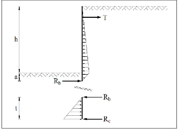
required to sum all the moments about the point O as shown in Figure 3-7, which is at the point of the anchor tie rod force, to equate the equation (3-25), rearranging to solve for the unknown length L4:

𝐿3₄+ 1.5𝐿2₄(𝑙₂+ 𝐿₂ + 𝐿₃) − [3𝑃(𝐿1+𝐿2+𝐿3)

𝛾′_𝐾

𝑝−𝐾𝑎 ] (3-25)

Figure 3-7: Anchored sheet pile penetrating a sandy soil (Das 1990)

The theoretical penetration depth can now be added = L3 + L4

into consideration. Thus, the actual penetrating depth of the sheet pile = 1.3 or 1.4Dtheoretical.

If a FOS is applied to Kp at the beginning of the design procedure, then the increase in theoretical depth is not required. According to Das (1990), the maximum theoretical moment to which the sheet pile will be subjected occurs at a depth between z = L1 and z = L1 + L2. The depth of zero shear force and hence maximum moment may be calculated by making a cut on the structure, analysing the structure as a beam and summing the moments around that point:

Point of zero shear = 0.5 × σ₁;L₁− 𝐹 +σ₁;(z − L₁)+ 0.5 × 𝐾𝑎𝛾′(z − L1)2 (3-26)

Thus, once the point of zero shear is determined, the maximum bending moment can easily be found.

Mmax= −(0.5 ×σ₁;L1)×[𝑥 +(L1⁄ )]₃ + 𝐹(𝑥 + 1)−σ1;x ×( 𝑥

2)− 0.5𝐾𝑎𝛾 ′_(𝑥2₎𝑥

3 (3-27) The solutions obtained for this example when using the analytical limit equilibrium methods are tabulated in Table 3-7.

Table 3-7: Analytical Results for Anchored Pile

Parameters Results

Length (m) L4 6.63

Theoretical Penetration Depth (m) Dt 2.22

Factor of Safety FOS 1.40

Actual Penetration Depth (m) Da 3.11

Total Wall Length (m) Ltot 12.11

Maximum Bending Moment (kN.m) Mmax 180

3.7

Anchored Sheet Pile Problem Description

The following example is solved analytically using the analytical design approach. The example is then solved in an Excel spread sheet developed in the paper so that the relevance of developing design tools for sheet pile walls can be understood.

line, the cohesion of the soil, the friction angle 𝜙 and the unit weight 𝛾 of the soil. For the example in Figure 3-8, the cantilever sheet pile wall is penetrating a sandy soil and therefore has zero cohesion. The friction angle 𝜙 and unit weight 𝛾 of the sandy soil were obtained from Das (1990).

Figure 3-8: Anchored sheet pile problem definition (Das 2007)

3.8

Development of Excel Spread Sheet for Anchor Wall Problem

The design of the Excel spread sheet was aimed at developing a tool to solve automatically the complex derived analytical equations, by requiring a user to enter known input data into clearly labelled cells.

Known Input Data

As the input data required were clearly explained for cantilevered sheet pile wall Excel spread sheet development, this shall not be repeated here, as the only difference is