BAYESIAN INFERENCE
WITH APPLICATIONS TO
FINITE POPULATION SAMPLING THEORY
Raymond Louis Hinde
Ä ‘Thesis S u S m itte d f o r the degree o f ‘D octor o f ‘Philosophy
o f the A u stra lia n O fational U n iversity
I hereby certify th a t this thesis does not contain any m aterial previously published or w ritten by any other person except w here due reference is made in the text.
T h is re s e a rc h h a s b een fu n d ed by an A u s tra lia n C om m onw ealth Public Service P o stg rad u ate S tudy A ward w ith the A ustralian B ureau of Statistics, for which I am very grateful.
Several years ago I worked for a while in an R&D area in the A ustralian B ureau of Statistics. At th a t tim e Dr Ray Cham bers was its supervisor and he fostered an attitude of interest in the fundam ental issues of sampling theory which generally go unnoticed. To him I owe a great debt of g ra titu d e , for th is re se a rc h is due e n tire ly to his help and encouragement a t th a t time.
This thesis is concerned with the foundations of statistics and how they in teract with the practical needs of finite population sampling theory. The current competing foundations are critically examined and compared. New foundations, which are a generalisation of the Bayesian foundations, are presented. They are applied to populations of random variables which are independently generated from Bernoulli, m ultiple B e rn o u lli, P oisson, n o rm a l, r e c ta n g u la r, L ap la ce an d gam m a distributions. The case of m ultiple linear regression is trea ted w ith and w ithout th e assum ption of norm al errors. P opulations of independent variables of no particular param etric form are also treated under various assum ptions which reflect realistic situ atio n s which occur in survey sampling. These include situations analogous to simple random sampling, , stratificatio n , w ithin stra tu m ratio estim ation, across s tra tu m ratio estim ation, probability proportional to size sam pling and m ultistage sampling. M ultistage sam pling is exam ined in the case of methodology used in designing the monthly Labour Force Survey ru n by the A ustralian Bureau of Statistics.
The diagram on the next page gives an idea of the interdependence between chapters. Chapter 15 however has been written so that it can be read at the outset in order to get a rough idea of where the thesis is going. Chapters 5 to 13 contain the difficult mathematical development. They consist mainly of theorems, the proofs of which need not be read in order to understand subsequent chapters. Chapters 5 to 12 are logically in parallel as they are different developments of the approach formulated in chapter 3. Chapters 5 and 9 contain the most important results and are the longest and most difficult chapters to read. The appendix to chapter 5 examines a related problem of the estimation of higher order moments of estimators derived from simple random samples and is not essential to the main ideas of this thesis. Chapter 13 applies some previous results to practical sampling situations. Chapters 14 and 15 are discussion and appraisal.
This thesis is concerned with two areas of statistics: Bayesian statistics and finite population sampling theory. Since few statisticians are intimately involved in both areas an attempt has been made in chapters 1 and 2 to make the thesis, at least in principle, self contained by giving any necessary background knowledge as well as outlining the issues of contention.
Notation is introduced informally in chapters 1 and 2. All such notation is defined again, more concisely, on the first pages of chapters 3 and 4. Any further notation is given in the chapters where it is specifically needed and it is required only for the chapter in which it is given.
10
Rectangular
\ \ z' _ \
8 \ Y2L 5
CONTENTS
Declaration i.
Acknowledgments iii.
Abstract iv.
How to Read This Thesis v.
1. BACKGROUND
1.1 Introduction 1
1.2 A Search for Truth? 1
1.3 The Controversy in Finite Population
Sampling Theory 4
1.4 Special Characteristics of Finite
Population Sampling Theory * 10
1.5 Robustness 12
1.6 The Role of Randomisation 13
1.7 Fiducialism, Overt and Covert 15
1.8 The Bayesian Approach to Sampling Theory 17
2. MOTIVATION
2.1 Vague Prior Knowledge 20
2.2 The Sample Mean Reflecting Vague Prior Knowledge 23
2.3 Conclusions and Aims 25
3. THE OBSERVER BASED FOUNDATIONS
3.1 Introduction 27
3.2 Bayes-consistency and Economy of Presentation 30
4. PRELIMINARIES
4.1 Notation 35
4.2 Characteristic Differential Equations 35
4.3 Results Deducible from Equation (2.3) 36
4.4 A Theorem 37
4.5 Bayesian Estimation 38
5. THE INFORMATIONLESS PROBABILITY STATE
5.1 Formulation 40
5.2 Finite Populations 44
5.3 Infinite Populations 49
5.4 Transformations of IPS Random Variables 50
APPENDIX
5.A.1 Higher Order Moments . 51
5.A.2 Higher Order Moments in the EPS 52
5.A.3 Higher Order Moments from a SRSWOR 53
6. THE BERNOULLI IPS 66
7. THE MULTIPLE BERNOULLI IPS 69
8. THE POISSON IPS 72
9. MULTIPLE LINEAR REGRESSION
9.1 Normal Errors 75
9.2 Discussion 89
10. THE RECTANGULAR IPS
10.1 a known 95
10.2 a and ß unknown 97
11. THE LAPLACE IPS
11.1 0 known 100
11.2 a known 102
11.3 0 and a unknown 104
12. THE GAMMA IPS
12.1 ß known 105
12.2 a known 109
12.3 a and ß unknown 110
j
13. SOME SAMPLING APPLICATIONS
13.1 Stratification 112
13.2 W ithin S tratum Ratio Estim ation 112 13.3 Across S tratum Ratio Estim ation 114 13.4 Probability Proportional to Size Sampling 116
13.5 M ultistage Sampling 123
14. PARADOXES
14.1 Introduction 129
14.2 Kolmogorov's Axioms 129
14.3 The M arginalisation Paradox 130
14.4 Strong Inconsistency 130
14.5 Transform ations of Random Variables 138
15. DISCUSSION
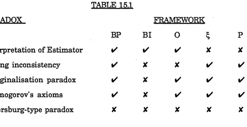
15.1 General 140
15.2 The Impact of Paradoxes 142
15.3 Versatility 144
15.4 Conclusions 145
CHAPTER 1
BACKGROUND
1.1 Introduction
T h at p a rt of the statistical world which concerns itself with the foundations of statistics is a m aelstrom of conflicting views. A casual observer can be ta k en aback by the in ten sity and aggression in the discussions accompanying some controversial papers. This section covers th is background, from th e point of view of a s ta tistic ia n prim arily concerned w ith finite population sampling theory. It is not comprehensive, ra th e r it focusses on highlighting concepts relevant to the theory developed in la te r chapters.
The disagreem ents between competing foundations of statistical inference are essentially disagreem ents between probabilistic concepts. Thus th e foundations of sta tistics will not be distinguished from the foundations of probability. There is no conflict about the m athem atics of probability. R ather, the conflict arises from th e conceptual aspects of probability concerned with its application and interpretation.
1.2 A Search for Truth ?
The developm ent of the foundations of probability theory can, p erhaps sim plistically, be considered to be a search for th e correct foundations of probability. In spite of all the differences of opinion between statisticians of different persuasions, there often appears to be a feeling of unity in th e search for the ultim ate answers, a feeling th a t in the end all factions will be in agreem ent, as one viewpoint proves, by overwhelming evidence, to be the correct viewpoint.
practical needs: that the form probability theory takes is by necessity determined by these needs rather than by the intellectual insights of the scholars of the day. From this point of view, there may be different correct foundations, depending on the particular application.
Hacking, in The Emergence Of Probability, suggests the latter view. Probability, as a mathematical science, emerged suddenly in the mid-seventeenth century. Hacking conjectures that its sudden prominence was due to a combination of the elimination of constraints as well as an emergence of needs. Significant constraints were: an obsession with predeterminism, piety and lack of an efficient system of numeration. When it did appear, it did so simultaneously in many different forms, fitting the many identified needs: "Huyghens wrote chiefly on aleatory problems. Leibniz began in an epistemological way, concerned with degrees of proof in law....The Port Royal Logic ...ends with a discussion of reasonable belief and credibility. G raunt’s O bservations .... is entirely dedicated to demography and the analysis of stable frequencies....Hudde and de Witt were doing the first actuarial science." (Hacking, 1975).
In particular, the notion of the duality of the concept of probability was immediately realised. One conceptualisation of probability is in the behaviour of long term frequencies of stochastic processes. Another is in quantifying one's beliefs. This duality is arguably the greatest single factor contributing to the confusion and disagreement between probabilists, and it exists to this day.
enters with the intention of placing his life savings on one spin of the wheel, he will not have any concern with long term frequencies as his interest is in the single spin. If he determines that the probability of a green 0 is 1/37, this is a quantification of his beliefs, a concept which need not be defined or justified in terms of long term frequencies.
While these two interpretations of the word probability exemplify the interpretations which will be considered in detail here, they are not the only ones. Consider a bookmaker putting odds on a horserace. He is not concerned with long term frequencies of the outcome of hypothetical reruns' of a race. Neither is he greatly concerned with his personal beliefs of each horse's chance of winning. His concern is usually in operating a 'Dutch book' where the odds are such that with the bets made, he will make a profit no matter what the outcome of the race.
Consider also the esoteric worlds of quantum mechanical probability (see Houston,1959, for a good introductory description) or the more recently developing study of 'ordered randomness' inherent in chaotic systems (Crutchfield et al, 1986).
These examples emphasise that it is not immediately evident that there is only one ultimately correct theory of probability. To put it another way, if one theory does emerge as the sole correct theory, it must be able to accomodate all of these different applications.
statistics, large and efficient bodies of knowledge based on different foundations have developed. Hacking also implies th a t champions of a p a rtic u la r philosophy are now, if anything, less to le ra n t of other philosophies. "Extrem ists of one school or another argue vigorously th a t the distinction is a sham, for there is only one kind of probability."
Why then does this conflict persist? Why do the different camps have th ere own accum ulated lite ra tu re seemingly in su late d from the wisdom of other camps? It would seem to be because there is simply no framework yet devised which satisfies the practical and conceptual needs of all the different areas of statistics. While this is supportive of Hacking's beliefs th a t there is no correct solution, it may be because no framework has been developed sufficiently far to gain the confidence of the bulk of statisticians in the major areas of statistical application. This is the belief of the author and this thesis represents an attem p t to help resolve the correct foundations to statistics.
-1.8 The Controversy in Finite Population Sampling Theory
In design based sampling theory the randomisation introduced by the sampling scheme is considered to be the sole source of probabilistic behaviour of the data. This is known as the randomisation principle. The properties of a random sample are considered in relation to the population of all possible samples. In doing so one can make quite sophisticated statem ents about the behaviour of sample outcomes: expectations, confidence intervals, approximate normality and so on, in the following m anner.
Suppose there is a finite population of N units. Associated with each unit is an unknown value y^. From this population a random sample s of size n is selected. Suppose the quantity of interest is T, the population total of the yj. The prefix p- will be used to denote design based concepts. If T* = T*(s) is an estimator of T then the p-expectation of T* is defined by
EPT* = X p(s).T*(s) (1.1)
' S € A
where p(s) is the probability of selecting the sample s and A is the set of all possible samples. The p-variance of T* is defined by
varp(T*) = X p^ T*(s) - EpT* )2 (1.2)
S €
The estimator T* is defined to be a p-unbiased estimator for T if EpT* = T. Similarly the estimator varp(T*) is defined to be a p-unbiased estimator for varp(T*) if Epvarp(T*) = varp(T*).
Consider the case where s is a simple random sample without replacement (SRSWOR). Then is the set of all groups of n distinct population elements, of which there are NCn. Each has p(s) = (NCn)-1. Direct evaluation then shows that
T = Nys (1.3)
varp(T) (1.4) is a p-unbiased estimator for varp(T').
In the superpopulation approach, selection probabilities are considered irrelevant once the sample is taken. Inference is instead conditioned on the observed sample. Randomisation is introduced by considering the population to be a random realisation from an infinitely large collection of possible populations, the superpopulation. The properties of the population are considered in relation to this superpopulation.
The prefix will be used to denote superpopulation based concepts. The ^-expectation and ^-variance of an estimator T* are determined by the form in which the superpopulation is modelled. For example the superpopulation model analogous to the design based SRSWOR scheme is the following:
E^Yj = p (unknown) (1.5)
var^(Yj) = a2 (unknown) (1.6)
Yj,Yk independent j*k. (1.7)
From this the ^-expectation of T' is found by E ^r = (N/n).2le3 EjiYj
= Np by (1.5). (1.8)
An estimator T* is defined to be a ^-unbiased estimator for T if E^T* = E^T. It can easily be shown by (1.5) that E^T = Np, so that T' is a ^-unbiased estimator for T.
If T* is a ^-unbiased estimator of T,then the ^-variance of T* is defined to be var^(T*-T) and the estimator var^(T*-T) is defined to be a ^-unbiased estimator for vars(T*-T) if E^vär^(T*—T) = var^(T*-T). It can be shown that for (1.5M1.7),
var^(T-T) = (N2/n).(l-n/N ).o2 (1.9)
expression in (1.9) so that it is a ^-unbiased estimator for var^(T*-T).
Observe that the finite population total T is considered to be a random variable. Observe furthermore that the for ye s are random variables, even after selection has taken place. Thus the superpopulation approach conditions on s but not on the sample values {ypes}.
Royall (1970, 1971) was one of many to rediscover the super population approach, but his development of it went much further than others. For a broad discussion of this framework the reader is referred to Cassel, Sämdal and Wretman (1977) and Royall (1983).
Many doubts about the design based approach have emerged over the years. It has been found to have many counter-intuitive consequences (Lahiri, 1968). On a more abstract level, Godambe (1955) showed that there is no unique minimum variance linear unbiased estimate within the class of linear estimates under the design based approach. To some extent the superpopulation approach has emerged as an alternative viewpoint which overcomes these problems. Its principle of conditioning on s is in direct contrast to the randomisation principle, so that the two approaches represent widely differing philosophies.
The variance estimator of the ratio estimator has, through initial investigations by Royall (1970, 1971) and Royall and Cumberland (1978, 1981), become a test case with which to debate the two approaches. The case for the design based approach has been backed by Hansen, Madow and Tepping (1983). This example will now be considered at length as it highlights issues which relate in principle to all estimators.
of the p—variance of T" is
varp(T") Cyt - f .xj)2
n - 1 (1.10)
Royall (1971) pointed out the following property of (1.10). When a random sample contains units with large Xj values then a large estimate of p-variance results. However it is just such a sample which, under the assumptions which make T" a sensible estimator, yields a good estimate of T. Similarly, if the Xj are small a bad estimate of T results, along with a low estimate of p-variance. Thus for a particular realisation, not only is the formula (1.10) irrelevant, but it reflects precisely the opposite of what it should. The superpopulation model which yields T" as the ^-unbiased estimator of T is
E^Yj = ßxj (ß unknown)
var^(Yj) = o 2Xj ( a2 unknown)
4
and (1.7). This gives
var (T-T”)
x(x-xs)
n —1
ie s
(yt - r.Xj)
(1.11)
(1.12)
(1.13)
where xs = sXj. The expression (1.13) is large when xs is small, and small when xs is large, properly reflecting the accuracy of the estimate.
This was analysed at length in two subsequent papers (Royall and Cumberland, 1978, 1981). The debate culminated in a paper by Hansen, Madow and Tepping (1983) which is essentially a response to the papers of Royall and Cumberland.
Arguably, the random isation process which generates a population is irre le v a n t once th e population exists ju s t as th e sam ple selection ra n d o m is a tio n is irre le v a n t once th e sam ple is selected. (The superpopulation approach, however, goes a long way to reducing the im pact of the resu ltin g conflicts w ith common sense). It is not new knowledge th a t the superpopulation approach shares these conceptual difficulties, and is subject to the same type of paradoxes, yet this is not explicitly brought out.
Consider the following example. Let me first stress, as Efron (1978) puts it: "The examples are artificially simple for the sake of humane presentation, but readers should be assured th a t real d ata are susceptible to the same disagreements". Suppose there is a Bernoulli population of size N=3. An SRSWOR of size n=2 is drawn and the sample values {0,1} are observed. It is required to estim ate T and compute an estim ate of the variance of-this estimator.
The design based approach gives the p-u n b iased estim ators of equations (1.3) and (1.4). This sample yields T'= 1.5 and varp(T') = 3/4. However, given the sample data, there are only two possible populations, {0,0,1} and {0,1,1}, ignoring ordering. The error of T' is either +1/2 or —1/2. In either case, the squared error is 1/4. However, the variance estim ator (1.4) gives an expected squared error of 3/4.
The superpopulation based model analogous to this design based scheme is the model:
E^Yj = 7i (1.14)
var^(Yj) = 7t(l—it) (1.15)
and (1.7), where k is the unknown Bernoulli proportion. This yields T' as
sense as the design based approach.
Presum ably th e design based ad h eren ts cannot use this as a counterattack as it would mean acknowledgement of the criticisms against th eir own foundations.
Another point of in terest is th a t the superpopulation approach is actually the more n a tu ra l extension, to finite populations, of frequentist techniques. It is therefore rath e r curious th a t it is viewed as the radical approach w ith support from only a minority of sam pling theorists. This is p artly for historical reasons as the design based approach was developed for finite population sampling fairly independently of the rest of statistics.
1.4 Special Characteristics of Finite Population
Sampling Theory
Foundational controversies in the context of finite population sam pling theory are ra th e r unusual because they are so dom inated by fre q u e n tis t approaches, w ith B ayesian m ethods very m uch in the background. W hat is so different about sampling theory th a t this occurs? It will be argued here th a t certain ch aracteristics of finite population sam pling makes the frequentist approach particularly appealing.
F irstly , the very fact of having a well defined finite lis t of population u n its allows a probability stru ctu re based solely on random selection from th a t list. This is appealing as the sta tistician can exert complete control over th e random process. This gives the design based approach the distinct advantage of apparent objectivity.
properties based on repeated selections can feel more natural, for the following reasons. The units in sample can be visualised as repeated selections of samples of size one. The samples drawn from each stratum can also be visualised as repeated samples. Surveys are often run repeatedly over a long period of time so that any particular sample outcome is one of a long string of outcomes. In these wrays it is intuitively easier to accept the properties of repeated selections as being relevant.
Consider again the estimator of variance of the ratio estimator. If, in a particular stratum, a sample with an unusually large x§ happens to be drawn, it does not particularly matter because this will quite likely be cancelled out by other strata where a disproportionately small xs is drawn. That is, over a large number of strata a central limit effect can occur.
Thirdly, an effect of taking large samples is that there is less need to utilise every bit of prior knowledge. A large sample design and estimation scheme can be intricately constructed so that it utilises most of the available prior knowledge. Combined with the effects of the sheer size of the sample, there can be negligible further gains from conditioning on the realised y^ in sample. This is one of the great strengths of both the design based and superpopulation approachs. Once the complexities of the sample design are mastered, the simplicity of the mathematics of random selection (either from the population or the superpopulation) allows estimation techniques which are often elegant and straightforward. (There are notable exceptions to this, for example with probability-proportional-to-size sampling: see Royall (1971) and the ensuing discussion with Koop (1971)). In running a large and complex survey, such practical considerations can outweigh theoretical considerations.
causal effects, such as whether smoking causes cancer. Then a model has to be used, with the model parameters quantifying the causal effects. Survey samples, on the other hand, are usually concerned with actual population characteristics, for example the incidence of cancer in a particular population in a particular year. Since a model is therefore not actually needed, then by Occam's razor it will be preferable to not have a model at all, all else being equal. This is easily achieved by the designed based approach.
While the first points indicate why frequentist methods may have been more likely to develop, they are not substantial supporting arguments. However, the two final characteristics, that it can be impractical to utilise every bit of prior knowledge and that a model can be superfluous, are substantial. These need to be addressed by any competing foundations.
1.5 Robustness
It is fairly unanimously agreed that robustness against incorrect modelling assumptions is an essential requirement of any inferential scheme.
model, there will be an inefficient design and the fact that an estimator is p-unbiased will not alleviate this fact.
Initially it appeared that the superpopulation approach was questionable because of its model dependence. However, the papers of Royall and Cumberland (1978, 1981) clearly showed that this is not a problem. Indeed, much of the more recent literature on superpopulation techniques is primarily concerned with robustness against model failure, for example Chambers (1986).
Robustness techniques are not within the scope of this thesis.
1.6 The Role of Randomisation
Design based theory considers th a t randomisation plays an essential part in providing insurance against model failure. Royall has repeatedly pointed out that it is balance that gives protection rather than randomisation. Royall and Herson (1973) and Scott, Brewer and Ho (1978) consider the effects of balance on robustness. Balance is quite difficult to define precisely since it means different things in different situations. The following rough definition will be sufficient here: a sample is balanced on x if the histogram of the x^ in s in some sense 'looks like' the histogram of the Xj of the population.
For example, the optimal sample in the case of the model (1.7), (1.11) and (1.12) will be the one which maximises xs as this minimises the ^-variance given by equation (1.13). However, if the model fails, then the ^-bias can be considerable, swamping the ^—variance. This risk can be overcome by balancing the sample on the x-values. However, approximate balance will generally be provide by randomisation. For this reason it is a debateable point wrhat actually provides the protection.
designs and estimators which are arithmetically similar. The arguments which still persist are more philosophical: does balance or randomisation ultimately provide the essential ingredient which ensures validity. This convergence of applied solutions suggests that there may ultimately be a set of foundations on which the different factions can agree.
Hansen et al (1983) raise im portant points which make randomisation highly desirable. Randomisation seems to be essential, but not for the primary reason of statistical validity, rather as a working practicality. Consider a large and complex survey being run by a government department. There is nothing in principle to stop even a complex design being effectively based on a purposive sample, provided it is taken with care. It needs to be balanced in a comprehensive way by, for example, balancing on different features of the x^. This will provide robustness against different forms of model breakdown. Also, if there are variables of interest other than yj, such balancing will provide good estimates for all the different variables. Balancing needs to be performed so that no systematic biases creep in.
Hansen et al (1983) also point out that "the acceptability and face validity of results that can be supported without having to defend assumptions....is often vital when....results are to be used for important public-policy actions or by opposing factions with different interests when the stakes are high." In certain situations this reason alone is enough to require randomisation. Putting all esoteric considerations aside, the instinctive feeling that only randomisation can ensure fairness is a strong motivator and provides a basis of operations that non-statisticians can agree upon.
Thus the two reasons for randomisation in large complex surveys are practicality and demonstrable impartiality.
These opinions agree broadly, if not completely, with those of Royall (1976b). Bayesians have also been concerned with the role of randomisation. Ericson (1969a) for example comes to similar conclusions.
1.7 Fiducialism, Overt and Covert
The previous sections have outlined the disagreements between competing frequentist approaches to sampling theory. As mentioned before, in broader statistical applications disagreements are more typically between frequentists and Bayesians. However, there is another important statistical philosophy, the principles of which can add clarification to the debate, specifically when we consider the interpretation of confidence intervals.
also known as fiducialism. It is unavoidably tied up with the practicality of making inferences within frequentist frameworks.
A fundamental aspect of the fiducial approach can be understood best by example. Suppose we have the following frequentist confidence interval for unknown ]p: Prob(y-1.96aA/n < p < y+1.96a/Vn) = .95, where y is a realised sample mean and a is known. This statement is saying that if the sample selection was repeated many times, with the resulting y placed into the inequalities, then 95% of the time the inequality would be true. It is a statement about the stochastic behaviour of y over repeated samples. This, however, is not what users want. Their interest is in making a stochastic statement about the value of p. The fiducial approach provides a formal mechamism for doing this by, quite simply, interpreting such a confidence interval as a statement about p, that given a realised y there is a 95% chance that the value of p is such that the inequality holds.
Great efforts have been made to develop the fiducial framework, for examples Fraser (1961) and Wilkinson (1977), but it has failed to gain much acceptance. While the fundamental principle of fiducialism is very compelling, it turns out that when it is formalised there develops a large quantity of conceptual baggage. For example, it does not conform to the Kolmogorov axioms of probability. It also generates logical paradoxes. While the paradoxes always appear to be resolvable, it is at the expense of creating further paradoxes and a general decrease in elegance and intuitive appeal. In short, the view taken here, in accordance with the significant majority, is that formal fiducial foundations simply do not work.
being estimated, and that for large enough samples the confidence interval is valid and short enough to provide as precise statements as desired about the value being estimated " (italics are my own). This epitomises the inevitable dilemma. For most practical applications, it is the likely value of the quantity being estimated that is of concern. When confronted with frequentist estimators, the user is forced into making a fiducial interpretation of some sort about the quantity being estimated, for the only formal statements that can be made concern the variability of estimates over repeated trials. When the authors say that the confidence interval provides a statement about the value being estimated, it is difficult to deny that this requires interpreting the confidence interval as a statement about the uncertainty of the estimated quantity. The frequentist framework passes the fiducial buck to the user and in doing so avoids the explicit occurence of conceptual problems.
For this reason the frequentist foundations to finite population sampling theory are arguably inadequate. While conceptual conflicts are initially avoided, they rise up later in applications, for example the ratio estimator discussed above.
1.8 Tike Bayesian Approach to Sampling Theory
We begin with a brief reminder of Bayesian principles. Consider a random variable Yj which has density function fXy^I 0) which depends upon the param eter vector 9. This 9 is generally unknown and any prior knowledge concerning its likely value is quantified by a prior density function f(9) for 9. If a sample ys is observed, this prior for 9 is updated to the posterior density function for 9 via Bayes' theorem:
fl9|ys) = fiys|Ö).fl9) / Jflys|9).fl9) dg (1.16) One can then produce the predictive distribution for further unobserved Yj
fljj|ys) =
J
flyjlö)-ftöjys)de
(i.i7 )Ericson (1969a) set out the following groundwork for the application of Bayesian methods to finite populations. Essentially it differs from most infinite population applications by the extra step of determining predictive distributions of quantities such as T after the posterior density of 9 is determined. A useful model is to consider each Yj to be independent conditional on the population parameter 9. Then the conditional density of the population vector of y-values, Y> given 9 is Il^ fiy ^ lg ) so that the joint prior for Y is
N
fly) = [ n f ly i|9 ) .f l9 ) .d 9 (1.18)
' § i=1
If a sample y s is observed then fig) is updated to f(9|ys) and the joint posterior of y is then
fly|y3) = J ftyi|0).ff9|ys).d0 (1.19)
e i«ss
assuming the elements of s in y match y s . It is then a matter of making transformations of random variables to determine such things as f(T|ys).
From this it is clear that Bayesian methods can be applied to finite populations without any conceptual difficulties. The development is purely mechanical. Since Ericson’s paper, Bayesian methods have been applied to some specific aspects of sampling theory. For examples, Malec and Sedransk (1985) consider multistage cluster sampling; Chiu and Sedransk (1986) consider the imputing of missing values; Rao and Ghangurde (1972) consider optimization; Hoadley (1969) considers categorical data; and Ghosh and Meeden (1986) look at empirical Bayes estimation.
CHAPTER 2
MOTIVATION
2.1 Vague Prior Knowledge
An aspect of Bayesian inference which is of crucial importance to this thesis is the Bayesian formulation of vague prior knowledge, and in particular the problems this seems to cause. These problems are well known and discussions can be found in Dawid, Stone and Zidek(1973), Bemardo(1979), Efron(1978), Wilkinson(1977) and Novick(1969). Vague prior knowledge is not a well defined concept. Indeed, this thesis will seek to give it a precise definition in particular situations with specific aims. At this point it will only be said that, in the Bayesian context, it refers to a prior density function f(0) which in some intuitive sense reflects the fact that little or nothing is known about 0. Such a prior will typically be wide and flat.
This concept is of particular relevance in the finite population context when there is very fine stratification. In such a situation, within a stratum there is very little information with which to distinguish between units.
As a preliminary, there is a central concept in Bayesian statistics th a t is often used in the representation of vague prior knowledge: exchangeability. This was introduced by deFinetti (1964). The random variables Y = {Y^,...,Y|sj} are exchangeable if all N! permutations of Y
have the same joint density function as
Y-
Exchangeability is adistributions, for example those given by (1.18) and (1.19).
Bayesian formulations of vague prior knowledge generally involve the use of improper priors. Improper priors are desirable because they look uninformative, for example, the uniform distribution on IR. Their main strength, however, is that they can lead to relatively tractable and intuitively appealing results. They can be chosen so that they lead to posterior densities which are both proper and very simple in form. For example Lindley and Smith (1972) use it in their three-staged multivariate linear model, as do Malec and Sedransk (1985) in a related development. Lindley later denounced the use of improper priors (Lindley, 1973). Nevertheless, in the case of a large and complex survey, 'hand fitting' a proper prior to every stratum is not really a practical solution and cannot be considered a realistic alternative to current frequentist techniques.
Improper priors have their own problems. First and foremost, they violate Kolmogorov's axioms. In spite of their paradoxes, frequentist methods work well in most practical situations. Therefore, an essential element in motivating applied statisticians to accept the Bayesian approach is that of conceptual elegance. There seems little gain in eliminating paradoxes only to replace them with probability densities that don't integrate to one.
th e form of a p rio r p ro b ab ility function. T his effect w as firs t described by
Stone a n d D aw id (1972) a n d in v estig ated fu rth e r by D aw id, Stone an d Zidek
(1973). S u d d e rth (1980) show ed t h a t th e p arad o x does n o t occur w hen proper
fin itely ad d itiv e p rio rs a re used.
T he follow ing exam ple is due to D aw id, Stone a n d Zidek (1973).
S u p p o se t h a t Y = (Y ^ ,...,Y r ) a re in d e p e n d e n t ra n d o m v a ria b le s w ith
d e n sity fu n ctio n s
where c*l is known, k can take the values {l,2,...,r—1} and r\ is unknown. If
the prior chosen for (tj,k) is «= 7r(K)dTi where 7t(l) + ... + 7t(r—1) = 1 then it follows that
w h ere = x^/x^ for i = l,...,r . I t is now easy to show t h a t th e re is no prior,
p ro p er or im p ro p er, for kw hich lead s to th e p o ste rio r given by (2.2).
A f u r th e r p a ra d o x t h a t a ris e s from im p ro p e r p rio rs is t h a t of
strong inconsistency . S to n e (1976) gives th e follow ing sim ple exam ple. If
Yj|0 ~ N (0,1) a n d th e im p ro p e r p rio r e49.d0 is a s s ig n e d to 0 th e n P r(0 > yj + 2 j yj) = 0 ( 2 ) re g a rd le s s of yj w hile P r(0 > + 2 | 0) = 0 ( - 2 )
re g a rd le ss of 0.
T h ere a p p ea rs to be a basic in co m p atib ility b etw een th e concept of
vague p rio r know ledge a n d th e specification of p rio r know ledge by w ay of a
p rio r d e n sity function. A d e n sity fu n ctio n co n tain s a lot of in fo rm atio n , for
e x a m p le in s p e c ify in g th e p a r a m e t r ic fo rm o f th e d is tr ib u tio n .
F u r th e r m o r e , a p rio r w h ic h m a y look in tu itiv e ly u n in fo rm a tiv e for a
v a ria b le c an look v e ry in fo rm a tiv e for m a n y fu n c tio n s of t h a t v a ria b le ffyihl,K) =
rj.exp{-r|y^} i = 1 ,...,k
cri.exp{-criyj} i = K +l,...,r
(2.1)
(Efron, 1973). For this reason the B ayesian approach is arguably too restrictiv e to be able to describe prio r knowledge in all conceivable situations.
Clearly it can be difficult to formulate a satisfactory representation of vague prior knowledge in the Bayesian approach, w hether by proper or im proper priors. Furtherm ore, it is in this particu lar situation th a t the frequentist m ethods are very powerful and elegant. For th is reason the B ayesian approach is considered inadequate when there is vague prior knowledge. This thesis addresses this problem and attem pts to resolve it.
2.2 The Sample Mean I&etflectmg Vague Prior Knowledge
In section 1.3 it was shown th a t in the design based approach, a simple random sample w ithout replacem ent leads to T' = N ys as the p-unbiased estim ator of the population total T. This is the number raised estim ator and is simply a scaling up of sample values to reflect the whole population. In the superpopulation approach, the model given by (1.5)-(1.7) leads to the num ber raised estim ator as the ^-unbiased estim ator of T.
C onsider an individual stra tu m of a large, finely stratified sample. Typically there will be known associated variables x^ which can be profitably included in the estim ation scheme, for exam ple by ratio estim ation or, if x is classificatory, by poststratification. However, the situation can arise in practice where there is such fine stratification th at negligible prior inform ation is given by the xi. P u t an o th er way, to d istin g u ish betw een u n its a t th is level would not be cost-efficient. Moreover, as far as the theoretical development of a theory of sampling is concerned, th is situation serves as a sta rtin g point from which more complex situations can be developed. In Bayesian term s, this requires a specification of vague prior knowledge.
reflect vague prior knowledge by use of the number raised estimator. (In fact, frequentists consider that it is the implementation of simple random sampling which reflects vague prior knowledge, with the number raised estimator being a consequence of this. The opinion of the author is that it is the number raised estimator that provides the intuitive motivation and that simple random sampling schemes were developed to support them). Whether this estimator is based on correct or incorrect foundations is not of primary importance. The important point is th at the number raised estimator is successfully used in practice. Furthermore, it does not waste any cost-effective prior knowledge when applied appropriately, for example in the context of fine stratification. Because of its well established usefulness and simplicity, theoretical considerations aside, any successful theory of finite population sampling must be able to incorporate the number raised estimator.
The number raised estimator is intuitively appealing even before it is formally justified by statistical theory. For this reason Bayesian techniques have been developed which attempt to reproduce it. While it can be approximated without difficulty, one must resort to improper priors to reproduce it precisely. Moreover, it is arguable that the number raised estimator is so intuitively compelling that it is worthwhile beginning with it as a premise and then deducing the characteristics of a subjective probability framework which would support it. This is in fact how this thesis developed.
More specifically, we can set
EYj|ys = ys for all je s (2.3)
where E . |ys denotes the Bayesian posterior expectation conditional on the
sample values ys. Then ETiys = sy{ + sys = Nys.
good', and are then evaluated empirically (see for example Andrews et al, 1972). N either is it u n n a tu ra l th a t foundations should be motivated by equations involving expectation operators, as opposed to beginning with Kolmogorov’s axioms of probability. Indeed, in m any ways defining axiom atic properties of th e expectation operator is the more n a tu ra l approach to the development of probability theory (Whittle,1970).
2.3 CoELcIuisions and Aims
In section 1.3 were discussed the paradoxes which arise when estim ators are not conditioned on the sample outcome. These occur due to the fiducial interpretations th a t the user of statistics is required to make, as discussed in section 1.7. Sim ilar paradoxes were shown to occur in the superpopulation approach, from precisely the sam e causes. For these reasons, the frequentist foundations are rejected as possible contenders for any universally 'correct' foundations as conjectured in section 1.2.
This leaves subjective probability. The B ayesian foundations overcome these paradoxes: for a broad discussion see Cornfield (1969) and for a lucid example see Lindley and Phillips (1976). Nevertheless, the strict confines of the Bayesian approach are rejected, as they currently stand, because they are inadequate to cope w ith real-w orld complex situations w here th e re is vague prior knowledge. B ayesian applications to such situ atio n s are eith e r im practical or else in te rn a lly in co n sisten t, as discussed in section 2.1.
co n sid ered e ith e r w ith in th e co n tex t of fin ite p o p u latio n sa m p lin g theory,
CHAPTER 3
THE OBSERVER BASED FOUNDATIONS
3.1 Irntrodmctio m
This chapter outlines the foundations of the proposed observer based approach to the foundations of statistics. They are a generalisation of the Bayesian foundations and the discussion here is largely concerned with identifying the differences from the Bayesian approach.
Suppose there exists a population of random variables {Yj} which
can have realisations {yj}. Let s denote a set of n labels associated with an observed sample. For all ie s, Yj = yj and denote the vector of sample observations {yjiie s} by yg. The symbol £ will denote a set of r labels of unobserved random variables and will denote the vector of {Yj:je Q. Let yg = Z ^y j/n the sample mean, ys = nyg the sample total and Y^ = Ij^Yj. Let £'u£"= £ be a partitioning of £ into mutually exclusive subsets of r' and r" elements respectively. Let T = ys + Y^ denote the total of the finite population, which has N = n + r elements. All density functions will usually be denoted simply by f and distribution functions by F. When this can cause ambiguities, appropriate subscripts will be used. The discussion below is equally applicable to continuous, discrete or mixed distributions, with appropriate changes in the formulae.
Difficulties occur when it is considered that there is little or no prior information about the vector 0. For example, the often used Bayesian prior for the mean |i of Bernoulli random variables is the Beta distribution. The prior knowledge th at Beta(a,b) represents can be interpreted as equivalent to having previously observed a sample of size a+b of which a are successes, where yj = 1 is a success'. It then follows that if there is no prior knowledge about ji then a Beta(0,0) prior density function is appropriate. Unfortunately Beta(0,0) is not a proper density function as it does not integrate to one. Such 'improper priors' can be used in practice, but there are many problems associated with their use, as discussed in section 2.1.
The observer based approach is a subjective probability framework which addresses these problems and produces well known and intuitively appealing estimators. Some are similar to estimators obtained by frequentist methods. Some are similar to those which can be obtained by Bayesian methods using improper priors, but without violating Kolmogrov's axioms.
It has been argued in section 2.1 that the difficulties in the Bayesian approach arise from the fact that a prior density function f(9) contains a lot of information and so the approach is inconsistent with the notion of vague prior knowledge. The observer based approach presents the idea that if there is substantial prior information, then the formulation of fig) is appropriate, but that in circumstances with less information a less stringent method of quantifying information is more appropriate. The approach incorporates two particular weakenings of the Bayesian approach: (i) there is no necessity for any prior density function f(9), either proper or improper, to exist and (ii) there can be a family of possible posterior density functions flyr|ys) for The approach does not allow the use of improper priors.
probability state (PS). A PS is any collection of equations (or inequalities) which imply a restriction on any relevant density functions. For example, a PS can be simply a Bayesian formulation of prior knowledge: a known param etric form f(yj|g) along with a known prior ft9) for 9. Thus the observer based framework generalises the Bayesian framework. When there is vague prior knowledge a PS can consist solely of constraints on the
posterior density function of For example, a PS can incorporate
equation (2.3). It may also include a parametric model for These will determine restrictions on the forms of f(y^|ys) and fly^lg) respectively.
Bayesian prior knowledge is very economically quantified by fig). The observer based approach is designed to also yield economical presentations of vague prior knowledge by way of a PS. Consider first the most straightforward but laborious way to have well defined posterior density functions for any y^|ys without the need for a prior fig) to exist. This is by explicitly specifying fly^|ys) for every set £ and every sample outcome ys. This can be demonstrated by example. For the Bernoulli!}!) case, treated in chapter 6, we could for example quantify vague prior knowledge of g = p by the following relations:
Yj|p ~ Ber(p), fo ra llje s, (3.1)
and if ys is any set of n sample observations satisfying ys = k * 0 or n then
Pr(y^|ys) = t+k"1Ct.'-t+n-1Cr_t/{n+r-1Cr.rCt} (3.2)
(3.2) are a consequence of the single constraint that fig) ~ Beta(0,0). However, the significant advantage of (3.2) is that Kolmogorov's axioms are not violated, for the simple reason that fig) and fiy^|ys) for ys = 0 or n are considered to not exist.
3.2 Bayes-consistemcy and Economy of Presentation
There are two obvious problems associated with this formulation. Firstly, there should be some way of ensuring that these explicitly defined posterior density functions fiy^|ys) are in some sense logically consistent with each other. Secondly, it is a very uneconomical and unconvincing way of expressing prior knowledge. These problems, however, can be overcome in the observer based approach without resorting to the use of an improper prior.
Consider the first problem. Logical consistency is ensured in the Bayesian approach by Bayes' theorem. By fixing fig), posterior density functions fiy^|ys) for every possible ys are an immediate consequence. One can then update this posterior density function to fiy^'|y^M,ys) when further information, y^», comes to hand by
Ky^'ly^">ys) = fiy^lys)/®[y^"lys) (3.3) recalling that £ = £’u£" is a partitioning of The consistency that Bayes' theorem ensures is that fiy ^ '|y ^ ",y s ) is independent of the order in which the elements of {ys,y^M} are observed. That is, fiy^iy^",ys) can be derived directly by (1.19) and the result will be the same as that obtained by updating fiy^|ys) to fiy r'!y ^ ',y s) through (3.3).
In the Bayesian framework, the conditional probability fiy^|ys) is defined by
conditional probabilities Pr(y^|ys) are defined by (3.2). Equation (3.4) is in ad eq u ate since f(ys ) will not always exist (when ys = 0 or n). Logical consistency between different posterior density functions of can then be obtained by requiring th a t the relation (3.3) hold, w henever all of its elem ents exist. This approach does not require th a t fly^O, fly^") and flys) exist. Similarly, if the Yj are of the known param etric form flyj|9) then we can require th a t
fl§ly£M>ys) = fl§lys) • flyjHS) / fly£Mlys)> (3.5) provided all the term s exist.
Any collection of posterior density functions which obey (3.3) and (3.5), w hen th e all term s in th e expressions exist, will be called B a v e s -c o n s is te n t. In th e observer based approach, Bayes-consistency provides the logical consistency between different density functions th a t Bayes' theorem and (3.4) provide in the Bayesian framework.
If all the term s in (3.3) and (3.5) are required to exist, they essentially am ount to Bayes' theorem. It is the provision th a t some terms may not exist th a t is the im portant distinction to bear in mind.
In the Bernoulli example above, given (3.1) and (3.2) it can be shown th a t (3.3) holds, w henever all the elem ents of (3.3) exist. A p articu lar advantage of Bayes-consistency is th a t it perm its a framework which avoids the restriction of dealing only w ith density functions which are assum ed to be of a particular param etric form, fly^lQ) (see chapter 5).
Bayes' theorem arises n atu ra lly from the likelihood principle which essentially states th a t all of the information in a sample ys th a t can be used for inferential purposes is contained in the likelihood function f(ys|9). For a formal definition and discussion see Cox and Hinkley (1974). This can be seen in equation (1.19) where the only occurrence of ys in the expression for fty|ys) is in the term fl9|ys), and since
then the only occurrence of ys is in f(ys|0).
The observer based approach adheres to the likelihood principle b ut with a proviso. In its current form the principle presupposes th a t the likelihood function both exists and is known. Since this need not be the case in the observer based foundations, the likelihood principle is adopted with the qualification in so far as the likelihood function exists and is known.
Define a solution to a PS to be a B ayes-consistent collection of functions ffy^ly-q) (and, if appropriate, fX01y^)) w here £ and r\ are non-intersecting sets of labels. The {y^,y-q} included in a solution is the dom ain of the solution. In the Bernoulli example above the domain of the solution to (3.1) and (3.2) is all Ky^ly^) for which y^ does not consist of only 0's or only l 's (i.e. ys * 0 or n). It is understood th a t domains of solutions have th e following property: if fly ^ly ^) is in the dom ain th en so is flyrlyrj^Tj')* I11 other words, if a sample ys determ ines a unique posterior density function for y^ then so will any sample which includes ys. It can be seen th a t if fly^|ys) is in a domain, then so are all the term s in (3.3).
The second problem associated w ith the PS defined by (3.1) and (3.2) is th a t it is cumbersome. Consider the constraint given by (2.3) which can be ta k en to rep resen t a state of vague prior knowledge. If this is included in a PS then it defines a family of fly^|ys)'s for every and ys by specifying th a t all the m arginal m eans of fly^|ys) are ys. It turns out th a t the PS defined by (2.3) and (3.1) has a unique solution which is given by (3.2) (see chapter 6). The formulation (2.3) plus (3.1) is ju st as economical as the Bayesian formulation of (3.1) plus the improper prior Beta(0,0) for q, which yields the same posterior densities.
3.3 D iscus siom.
associated with (3.1) and (3.2).
Equation (2.3) is not the only constraint that can be used to quantify vague prior knowledge, for example the median of ys can be used instead of the mean. While (2.3) has a certain amount of arbitrariness, it has much intuitive appeal. A model used to describe data is rarely the only feasible one, but this does not detract from its usefulness.
Intuitively appealing PS's such as that defined by (2.3) and (3.1) can be formulated for a wide variety of situations of vague prior knowledge. This thesis presents several such probability states and discusses their implications. In particular it will be shown th at the observer based framework overcomes the theoretical difficulties found in the analogous Bayesian solutions and has a versatility in dealing with cases of very weak prior knowledge which has no obvious analogy in Bayesian theory. Estimators and confidence intervals will be obtained which are identical, or very similar, in form to frequentist solutions.
An explanation is needed in the interpretation of probabilities and expectations in the observer based approach. Probability functions such as f(yj|0) or F(0|ys) are interpreted exactly as they are in the Bayesian approach. An expectation operator admits a family of possible posterior probability functions. For example, equation (2.3) is saying that the random variable Yj has a density function flyj|ys) which is not precisely known but which has mean yg. A probability state can also admit a family of possible solutions. One of the strengths of this approach, however, is that many parsimonious probability states have a unique solution which can be determined.
a n y p rio r d e n sity fu n ctio n a n d by allow ing a fam ily of possible po sterio rs.
P rio r know ledge is in s te a d fo rm u la te d by a p ro b a b ility s ta te . T h ese can
produce p o ste rio r p ro p e rtie s w hich r e s u lt from th e u se of im p ro p e r p riors,
b u t w hich do n o t violate K olm ogorov's axiom s. Logical consistency a n d th e
l ik e l ih o o d p r i n c i p l e a r e m a i n t a i n e d i n t h e f r a m e w o r k b y
CHAPTER 4
PRELIMINARIES
4.1 Notation
Some preliminary notation is given at the beginning of chapter 3. This section outlines further notation that is adopted throughout the remainder of this thesis. Extensions to this notation are sometimes given within specific chapters.
Many of the proofs are concerned with moments. If r\ is any set of m population units, some of which may be in sample and some not, define:
Mt,ri “ Zjer| DjV m
^t,s = ®qjys
where = ZjeTjYj/m. As a general rule, an upper case symbol denotes a random variable while the corresponding lower case symbol denotes a realisation. For exam ples d^s = y^ - y s for any is s and m ^ s = SiG s(y^-ys)Vn. A subscript such as s+j denotes the union of s and j, for example M2>s+j = (su j)(Yr Ys+j)2/(n+l).
Pr(e) denotes the discrete probability of the event e.
4.2 Characteristic Differential Equations
Many of the probability states that are investigated in this thesis yield unique solutions. Such probability states include the constraint that the distribution of Yj|9 has the known parametric form flyj|9) for all j<es, with the Yj|9 independent. The following formula is very useful in deducing a unique solution. Let g(9) be an arbitrary function of 9. Then
= J
g(0).f(yj|0).dF(9|ys) / flyj|ys)by Bayes—consistency
= E{g(0).flyj|0)|ys} / flyj|ys) (4.1)
This equation can be differentiated with respect to yj. It tu rn s out th a t by judicious choice of the functions g(9), and by incorporating the constraints of the PS, this differentiation process can result in an ordinary differential equation based on either flyj|ys) or fl9|ys). The advantage th a t this gives is th a t existence and uniqueness results of ordinary differential equations are well established so th a t a unique solution to the PS can th en be easily deduced. Such uniqueness and existence resu lts can be found in any standard textbook, for example Boyce and DiPrima (1969).
In the case of a discrete density function, equation (4.1) is then expressed as
If Yj is in teg er valued, judicious choice of g(9) can lead to recursive relations betw een P r(yj|ys ) and P r(y j+ l|y s) which th en yield a unique solution.
4.3 R esults DeduciM© from E quation (2.3)
An im m ediate consequence of Bayes—consistency is th a t if, for some function g(.), Eg(y^)|ys is known then
This relation, and variations of it, are useful in deducing properties of a PS. This is because PS's are generally defined in term s of expectations, such as equation (2.3). This technique has been used w ithin th e B ayesian framework, by Ericson (1969b, 1970) to determ ine the form of posterior m eans and variances and by G oldstein (1975) to uniquely determ ine
(4.2)
E g ( lc)|ys = E{Eg(Ic)IY Csys} ly s. (4.3)
moments of prior distributions.
cov(Yj,Yk|ys) = E (Y j-y s){E(Yk - y s)|Yj,ys}|ys j*k*j,kes,
= var(Yj|ys) / (n+1) (4.4)
since by (2.3), EYk |Yj,ys = (Yj+ys)/(n+l). Similarly, cov(Yj,Yk |ys) = var(Yk|ys)/(n+l) so that it follows that var(Yj|ys) is independent of j and cov(Yj,Yk|ys) is independent of both j and k. Also,
ETlys = ^ ie s^ i + ^jgsEYj|ys
= T by (2.1) (4.5)
where T = Nys as given in equation (1.3), var(T]ys) = v a r 0 ^ sYj|ys)
= I j g s var(Yj|ys) + £ j g s I k g Scov(Yj,Yk |y s ) j*k
= N2(l-n/N)var(Yj|ys)/(n+l) by (4.4). (4.6)
If we consider each Yj to be independently generated from a distribution with unknown mean p, then since EYj|ys = E{EYj|p}|ys = Ep|yg then by (2.3):
Epiys = ys. (4-?)
4.4 A Theorem
Theorem 4,1: Suppose a probability state includes the constraint that flyj|9) is given and the Yj| 9 are independent. Then for any solution to the probability state there exists a function h(9) of 9 so that for any sample, s,
f(9|ys) ~ f(ys|9).h(9) (4.8)
whenever the elements in (4.8) exist. The constant of proportionality is a function of ys only.
Proof: By Bayes-consistency
R0|ys+j) = ^ y s + j l ^ - ^ ^ ^ i ^ s + j ) (4.10) Equating the right hand sides of (4.9) and (4.10) yields
(4.11) satisfying equation (4.8). From equations (4.10) and (4.11) it can be seen th at h(9) does not change as the sample size increases so th a t h(9) in (4.8) is the same for all possible samples.■
The function h(9) performs the same role as a prior, either proper or improper, does in the B ayesian framework. If h(9) tu rn s out to be a proper density function, it can be interpreted as such in the observer based frame. If im proper, it is in terp reted as no more th a n a function which characterises the solution.
Thus the search for a solution to a probability state can be mechanically equivalent to the search for a prior for 9. However, w ith the exception of the Laplace IPS (g known) of section 11.2, the function h(9) is
not explicitly sought. This is because there are other more elegant methods of finding solutions. Also, many of the probability states do not meet the conditions of theorem 4.1. In this instance there is no h(9).
4.5 B a y e sia n E stim a tio n
E stim ators used in frequentist frameworks are typically chosen from among the collection of p— or ^-u n b iased estim ators. The actual choice is usually determ ined by optimizing on some quantity, for example by m inim izing p— or variance. W here u n b iasedness is not easily achieved a near-unbiased estim ator is chosen.
CHAPTER 5
THE INFORMATIONLESS
PROBABILITY STATE
5.1 Formnilatiom
The Informationless Probability State (IPS) which will be defined here provides a characterisation of no prior knowledge of random variables
Yj-Firstly, the constraint (2.3) is appropriate for a model exhibiting a lack of knowledge of Yj. This can be contrasted with the Bayesian use of informationless priors over R. Suitable priors will have a high variance and be fairly uniform over a wide range. This is done to enhance the resulting posterior estimator's data dependence, so that for example the posterior mean will be close to the sample mean. The desirability of this property is made explicit by (2.3). Bayesians can obtain (2.3) by the improper prior p~N(0,°o), which is interpreted as the limit as o2 -» °° of ji ~ N(0,a2).
Secondly, when there are n units in the sample it is reasonable that one should be able to simultaneously estimate n posterior functions of
Yj. A suitable choice of functions are the posterior moments of Yj up to order n. The IPS thus contains the constraints
h fi = at,n mt,s fo rt =2,.... n (5.1)
where a^n is a non-zero constant depending on only t and n, for all ys satisfying m2 s * 0 (so th at the posterior density functions are not degenerate). This form of X,^s suggests itself because it is translation
invariant and symmetric in the ys. Also, forms of which involve