Few-mode optical waveguides and their study by the four-photon mixing process

FOUR-PHOTON MIXING PROCESS

Stephen John Garth

A thesis submitted for the degree of

Doctor of Philosophy

at the Australian National University

Canberra

1. page 12. Footnote to eqn. (2.14)

"Eqn. (2.14) is exact, but we note that it was derived by refering th field components to a fixed cartesian coordinate system".

2. page 25. Above eqn. (2.40)

The relation re tween J i n n2 and profile shape should be " V,. In n2 = - 2A V , f "

~ t ~t

3. page 26. Eqn. (2.42)

To avoid confusion, l in eqn. (2.42) should be replaced by s, with th following comment:

"where ds = p d<f> is an element of arc length of the boundary interface".

4. page 35. Eqn. (2A.3) Eqn. (2A.3) should be:

« ( V t " ) + k£ +i(w ) )

2 K£ (W)

where the field in the cladding is given by y = K^(W) ".

5. page 43. Addition to last paragraph.

"(See ref. [7] for a complete discussion of the feasibility of using th] system for local area networks. We are only concerned with dispersic properties in this discussion)."

6. page 44. Eqn. (3.2)

Australian National University between February 1983 and March 1986, while I was enrolled for the degree Doctor of Philosophy.

Professor C. Pask supervised the research, but unless specifically disowned, the material presented herein is my own.

None of the work presented here has ever been submitted for any other degree at this or any ocher institution of learning.

Publications

[1] S.J. Garth and C. Pask, "Properties of modes on perturbed fibers" Electron. Letters, 22, pp. 22-28 (1986).

[2] S.J. Garth and C. Pask, "Four-photon mixing and dispersion in single-mode fibers"

Optics Letters, JJ_, pp. 380-382 (1986).

[3] S.J. Garth, "Modes on a bent optical waveguide" IEE Proc. Pt. J., (in press)

[4] S.J. Garth, "Birefringence in bent single-mode fibers' IEEE J. Lightwave Tech., (in press)

[5] S.J. Garth, "Fields in a bent single-mode fiber" Electron. Letters, (submitted)

Papers in preparation:

[6] C. Pask and S.J. Garth, "Comparison of focal and afocal lens systems

in insect eyes"

[7] S.J. Garth, C. Pask and G.E. Rosman, "Four-photon mixing in bent

few-mode optical fibers"

[8] S.J. Garth, C. Pask and R.A. Sammut, "Single-mode fibers operating

Acknowledgements

Mow that the task of writing up this thesis is over I can sit back and get into the really important things in life - such as writing these acknowledgements. They say that a man's worth is the sum of all the people he has known. If so, then over the last four years I have indeed been fortunate.

It's not possible for me to fully express my thanks and gratitude to Colin Pask, except to say no one could have a finer supervisor and friend. Colin has been a constant source of encouragement and guidance. His understanding of, and committment to, research students is without parallel, and he has made my time in a research environment an enjoyable and rewarding experience. I have gained much more than just a degree by my association with Colin.

I owe an enormous debt of gratitude to Barry Minham, the founding head of the Department. Barry is the driving force behind a dynamic, exciting, and friendly department. He has been a great inspiration to me, and I value his advice and friendship.

For the last year I have been a Teaching Fellow in ehe Department of Mathematics at the Australian Defence Force Academy. Under Colin's zestful leadership this is a friendly and active Department, and I have enjoyed the year tremendously. I would like to thank Rowland Sammut for many helpful discussions.

I would especially like to thank Gavan Rosman, of the Telecom Research Labs in Melbourne, who introduced me to the problem of four-photon mixing in optical fibers. Later he showed me around the Labs, and allowed me to participate in the re-creation of some of the experimental results that are presented here.

I owe much to my typist, and friend, the lovely Diana. Her dedication, ability and sensational body are without question, and the layout of this thesis is due to her. I thank Julie and Shiu for providing an efficient computer service.

FEW-MODE OPTICAL WAVEGUIDES and their study by

THE FOUR-PHOTON MIXING PROCESS

The design and use of optical fibers for communications systems or sensing devices requires an understanding of the properties of modal fields. This thesis theoretically examines mode characteristics on optical fibers where the symmetry has been broken, especially in the cases of fibers that are uniformly bent and those that have arbitrary shaped core cross-sections.

In general the higher-order modes of these fibers are strongly affected, as they are dependent on symmetry, and a birefringence in the fundamental mode originates. Corrections to the fields and propagation constants of the unperturbed fiber are found by several perturbation methods. The relation between symmetry and polarization effects is discussed in detail.

In order to examine the modal characteristics of these fibers the theory of stimulated four-photon mixing is employed. This non-linear optics effect generates multiple new output frequencies that are symmetrically shifted above and below the input frequency. The process occurs strongly when it is- phase-matched.

A study of the resulting shifts in optical frequencies on few-mode fibers gives information on the symmetry and magnitude of fiber perturbations, and thus the theoretical results are available for confirmation by experiment. Some experimental results that have been performed by other researchers are included.

Motes on Text

References are labelled within each Chapter by square brackets, i.e. [12]. A list of references is found at the end of each Chapter. Back- references to past Chapters are given by:

See ref. [3-9]. This means see reference [9] of Chapter 3.

CONTENTS

Declaration i

Publications ii

Acknowledgements iii

Abstract v

Motes on text vi

1. Introduction 1

2. Properties of Few-Mode Optical Waveguides 4

3. Dispersion of Light in Glass Optical Fibers 40

4. The Stimulated Four-Photon Mixing Process 69

5. Phase-Matched Processes 90

6. Modes on a Perturbed Optical Fiber 118

7. Modes on a Bent Optical Waveguide 155

8. The Gaussian Approximation for Bent Fibers 203

CHAPTER 1

INTRODUCTION

Optical fibers are used extensively for long- and short-range communication systems, as well as in high-sensitivity measuring devices. In order to fully utilize the potential of such systems one needs to determine and understand the fiber characteristics. This thesis theoretically examines changes to the electromagnetic fields when the fiber is perturbed from the ideal case, and examines the use of a non­ linear optics process in order to measure such changes.

We are principally concerned with few-mode optical fibers that are perturbed by (i) uniform bending, and (ii) a non-circular core cross-section. The perturbations can be measured by the stimulated four- photon mixing process, a non-linear effect that reveals information about not only waveguide characteristics, but material characteristics as well. The fiber material properties are very important in the design and application of single-mode fibers for long distance communication systems.

that are used throughout is presented, as well as a review of the Gaussian approximation, which is used to simplify the description of the modal fields.

In Chapter 3 the dispersion properties of glass fiber waveguides

art * p^rvio{\

-4-3- examined. The ■ dispersion- consists of material and waveguide causes

contributions, and -d escribes— pulse spreading due to the modal characteristics as well as the dependence of the refractive index on wavelength. Curves that describe the group delay and chromatic dispersion are presented for the different profiles.

A very important design consideration for single-mode fibers is the zero-dispersion wavelength, where material and waveguide contributions to the dispersion cancel. The design and application of fibers operating at this wavelength is discussed. The practical implications of operating such a fiber at lower wavelengths than they are designed for is

investigated.

In Chapter 4 the stimulated four-photon mixing process in optical fibers is reviewed. This non-linear optics effect generates multiple new frequencies at the output of the fiber. These new frequencies are symmetrically shifted below and above the input (or pump) frequency. The process occurs strongly when it is phase-matched.

Chapter 5 deals with this phase-matched condition, and it is shown that the resulting frequency shift reveals information on the material and modal properties of few-mode fibers. Phase-matching on single-mode fibers offers a way to examine the total dispersion

characteristics of the fiber.

these fibers are strongly affected, as they are dependent on symmetry, and a birefringence originates in the fundamental mode. The relation between symmetry and polarization effects is discussed in detail. A study of frequency shifts on these fibers gives information on the symmetry and magnitude of the perturbations.

Profiles that are perturbed by having a depressed refractive index profile (or dip) are also examined. In this case the symmetry is not broken but modal characteristics, such as group delay, are strongly affected. We use the theory of four-photon mixing to study these changes, and compare our results to experimental data.

Chapter 7 examines the modal characteristics on waveguides that are uniformly bent. This form of perturbation also breaks the degeneracy of the higher-order modes and creates a birefringence between the orthogonally polarized fundamental modes. 3y using the theory of four- photon mixing the theoretical prediction of mode splitting is confirmed by experimental results.

Chapter 8 attempts to simplify the description of mode propagation on bent fibers by using the Gaussian approximation for modal fields. The simple forms of the approximation also allow an investigation of the perturbation theory used to analyse bends. Finally, experimental results showing the shift of the peak intensity of the electric field due to the bend, in regions where the usual perturbation theory breaks down,

CHAPTER 2

PROPERTIES OF FEW MODE OPTICAL WAVEGUIDES

1. Introduction

2. Basic Theory

(a) The Vector Wave Equation (b) Polarization Properties (c) Modal Parameters

3. Modal Characteristics

(a) Singly-Clad Step-Profile Fiber (b) Singly-Clad Power-Law Profile Fiber (c) Doubly-Clad Step-Profile Fiber

4. Polarization Corrections to the Step-Profile Fiber

5. Gaussian Approximation to Modal Fields

6. Appendix

(i) Zero-finding routine for functions

(ii) Eigenvalues and fields for arbitrary profiles

CHAPTER 2

FEW-MODE OPTICAL WAVEGUIDES

1. Introduction

In this chapter we lay the foundations of the waveguide theory a r e that will be used throughout this work. While parts of this chapter 4s- essentially a review of standard theory (see reference (1]), we present some results which are not available elsewhere.

Throughout this work we are concerned with three types of waveguide structures ; (1) the basic singly-clad step-index (or rectangular-profile) fiber; (2) the singly-clad power-law profile fiber; and (3) the doubly-clad (W-type) step-index fiber. These three profiles are shown in Figure 2.2.

We begin at the beginning: Maxwell's equations and the homogeneous vector wave equations. We then invoke an approximation to solve the wave equations. This approximation, called the "weakly-guiding limit", is the basis of the theoretical analysis of waveguides presented here, and is related to the polarization properties of the waveguide. The details and significance of this approximation are discussed.

We then present the mode characteristics of the three fiber models we are investigating. We write down the solution to the wave equation, called the modal field, for the solvable cases and detail the numerical solution for the other cases. We present curves which give the eigenvalue and cut-off characteristics of the respective waveguide structures.

We then examine the polarization corrections in more detail, and as an example consider the singly-clad step-profile fiber. We show how the vector fields can be constructed from the scalar fields, and how these corrections describe the polarization properties of the fiber.

In the next section we show how approximations to the "weakly- guiding" waveguide solutions can be made by making use of the fact that the fundamental mode field is Gaussian in shape. Simple analytic solutions result for many waveguide parameters, and the approximation can be extended to describe higher-order modes as well. We examine and discuss the accuracy of the Gaussian approximation in relation to the mode characteristics we will be concerned with.

2. Basic Theory

(a) The Vector Wave Equation

In this section we quickly review the fundamental equations for an electromagnetic analysis of optical waveguides. Maxwell's equations in non-magnetic, homogeneous and isotropic source-free media are [2]

V x E + u 0 3H/3t = 0 V x H - 3D/3t = 0

~ ~ ~ (2.1)

V - D = 0 V • H = °

where E and H are the electric and magnetic fields, respectively, u 0 is the free-space permeability, and the electric displacement, D , is related to the electric field by

D = e0 5 + P (2.2)

£0 is the free-space dielectric constant and ? is the electric polarization, which in linear media is given by

P = e0 X E (2.3)

i Scalar

where x is the electric susceptibility -tensor-. Combining eqns.(2.2) and

(2.3) we have

D = e0 n 2 E (2.4)

where the refractive index n(x,y,z) is related to the susceptability

n(x,y,z) = (1 + x)1/2 (2.5)

We shall be concerned with electric and magnetic fields "hat have an implicit time dependence exp(-iwt) , so that the time derivatives of

eqn.(2.1) can be replaced by factors of icu = ike , where

c = (e0 u 0 )- 1/2 is the speed of light in free space and

k = 2ir/X (2.6)

is the free space wavenumber, where X is the wavelength of light in free space.

If we eliminate either the electric or magnetic fields from eqn5, (2.1) we obtain, with the use of eqn.(2.4), the homogeneous vector wave equations;

{V 2 + n 2k 2} E = - v(E • 7

In

{v2 + n 2k 2} H = (7 x H) x 7 in n 2 (2.7b)

If the refractive index profile does not vary with longitudinal distance z along the waveguide, so that n = n(x,y), then the electric and magnetic

a

fields can be expressed in the separable form

E = Ie. + e z ) exp(i3z)

~ t z ~ (2.8a)

where 3 is called the propagation constant, z is the unit vector parallel to the waveguide axis, and subscripts t and z denote the transverse and longitudinal field components. 3y substituting eqn. (2.8) into eqn. (2.1), and comparing longitudinal and transverse field components, relationships between the field components e , , e , h, and h are obtained.

'** L/ Z ~ Ü Z

The operator 7 2 in eqn. (2.7) is a vector operator, and couples the field components in an arbitrary coordinate system, as we shall see in Chapter 7, when we deal with bent optical fibers. However, if the field components are specified relative to fixed cartesian coordinates, ie.,

e, = e x + e y ~t x - y 1

h,_ = h x + h y ~t x ~ y ~

(2.9)

then this coupling does not occur and the vector operation is replaced by the scalar Laplacian 7 2 .

Substituting eqn. (2.8) into eqn. (2.7), separating longitudinal and transverse components, then we have the vector wave equation of the

transverse electric field [1]

[7j + n2k2 - 32) e, = - ?t(et •

7t In n2)

(2.10)

where e, are defined by eqn. (2.9), n = n(x,y) and

~ 3 f ~ a f

? t f = ~ 3X + l 3y

7 2 f = --- 4-3 2f 3 2 f

t

(b) Polarization Properties

There are few exact solutions to eqn. (2.10), and so we must use approximation methods to obtain the field and propagtion constant. The term on the right-side of eqn. (2.10) is called the vector correction term, and describes the polarization properties of the electric field. This correction term is due to the fact that the refractive index varies over the cross-section of the fiber.

In an infinite medium of constant refractive index the electric field would be a plane wave whose initial polarization state would be maintained as it propagates through the medium. The vector correction term changes the electric field so that its polarization state rotates as it propagates along the fiber.

The "weakly-guiding” approximation makes use of the fact that the difference between the refractive index of the core and cladding regions is negligibly small, so that the vector correction term in eqn.

neql^cHci

(2.10) can be se t equal to aero -[3,4]. In other words, if the refractive indicies are nearly equal, the slight boundary difference maintains total internal reflection, so light is still guided by the waveguide, but the medium is virtually homogeneous as far as polarization effects are concerned, and the wave is essentially plane polarized. The modes are said to be "linearly-polarized" [4].

If we set the vector-correction term in eqn. (2.10) to zero then

we obtain the scalar wave equation [5,6]

{V2 + n2k2 - 32} £ = 0 (2.11)

U v'

is kn „ < 3 < kn where n and n „ are the maximum values of the

CÄ, CO CO cl

refractive index in the core and cladding respectively. Thus the variation of 3 on weakly-guiding waveguides is very narrow and we set

3 = kn = kn n (2.12)

co cl

By knowing only eu the modal fields are fully specified. The waves are very nearly plane waves and e7 = 0, h^ = 0 .

The scalar wave equation (2.11) will be the basis of our theoretical analysis of mode properties in this work, and later we will see that this equation will be sufficient to describe the higher-order modes of perturbed optical fibers. A. solution of the scalar wave equation represents a modal field whose intial state of polarization is maintained over the entire length of the fiber. However, in general polarization properties are important, and describe how the polarization state changes as the mode propagates through the fiber. In particular, we shall see in Capters 6 and 7 that these polarization effects are essential to describe birefringence phenomena. These effects can be included by adding a correction term to the scalar propagation constant (7,8]. The proper modal fields are then given by the scalar solution plus correction term.

We

32- 32 = ! e, • 7. fe. • 7. in n 2} dA/ j i • e. dA (2.13) w ^ ~ t - c L ~ t t J J ,, -1 - c

CO CO

The terms involving 7 2 vanish, as we can transform the area integral over z

these terms into a line integral using Green's theorem: fe. • 7 2 e. - e, • 7 2 i ) dA

J . ^~t t ~t ~c t A

CO

= 6 {5. v u • eu - e, 7. • 5. } • n da - „ L~c ~t -t ~t ~t ~tJ

i

CD

where I is the Derimeter of A and n is the unit outward normal on 1 in

CO CO — CO

the plane of A . Because the fields of bound modes and their derivatives co

decay exponentially to zero at large distances from the waveguide the line integral vanishes.

Using the vector identity

h ■

(f M s

f V + 4t

•

zt

f

and noting that the area integral over f 7U • e_ can be transformed into a line integral, which will vanish, the integrand in the numerator of eqn. (2.13) can be re-written and we obtain

32 - § 2 = - (yu • e } e • 7 in n 2 dA/ J 5 • e. dA (2.14)

CO CD

We use this equation to show the vector corrections for the modes of a

(c) Modal Parameters

We now introduce the normalized parameters that we will use throughout this work. The normalized frequency is

V = ko n (2A)1/2 (2.15)

co^ '

where k = 2tt/\, p is the fiber radius (or half-width of a rectangular guide) and the profile-height is defined to be

A =

\

(2.16) * (n - n 1/n

Following our discussion in the previous section, the ''weakly-guiding" approximation may be described as the A 0 limit [4]. Throughout this work we assume that the refractive index in the cladding is a constant and extends to infinity, and the variation of refractive index in the core is given by

n 2( x , y ) = n 2 ( 1 - 2 A f ) (2.17)

7

J

where f describes the shape of the profile.

The normalized eigenvalues are defined to be [1]

U 2 = p 2(k2n 2q - 32) (2.18a)

W 2 = p 2f62 - k 2n 2 ) (2.18b)

so that U 2 + W 2 = V 2 .

Fig. 2.1 A circularly symmetric fiber, which is unbounded in the r- and z-directions. The core radius is o , the normalized radius is

R = r/p , and n(r) is the refractive index profile.

(a)

(b)

15— ;

3. Modal Characteristics

We now have the basic equations necessary to describe the behaviour of light propagating in optical waveguides. The equations are general and apply to waveguides of any profile shape or cross-sectional shape.

Throughout this work we will deal with 3 types of fibers; the singly-clad step- and clad power-law profile fibers, and the doubly-clad step-profile fiber. We will consider a circularly-symmetric cross- section, so that the scalar wave equation (2.11) can be written as

f— + - — + — — + k 2n 2 - 3 2) o = 0 (2.19)

3r2 r 3r r 2

where the scalar Laplacian has been written in cylindrical polar coordinates and b = e x or i

x - y y • ’4) can be expressed in the separable form

= F a(R) r C O S £<t>| Lsin 2,ct>J

(2.20)

where (cos refer to ie^ n } modes, l - 0,1,.... , and we have introduced the normalized radial coordinate R = r/o . We will use this normalized coordinate throughout this work. The radial function F (R) is

4

K«,

then the solution to-be differential equation

( i — + - + 'J2 . v 2 f(R ) ) F (R) = 0 (2.21)

^ R 2 R R2 1

(a) Singly-Clad Step-Profile Fiber

This profile shape, shown in figure 2.2(a) represents a fiber with a constant refractive index in the core and a constant refractive

index in the cladding, and with respect to eqn. (2.17) is specified by

f(R) = 0 < R < 1

R > 1 (2.22)

The solution to equation (2.21) is then given by

J 1(UR)/Jl(U) , 0 < R < 1

F (R) = { (2.23)

K^(WR)/K^(W) _{, R} > 1

where J and K are the Bessel and modified Bessel functions. The eigenvalues U and W can be determined by matching the field and its first derivative at the fiber boundary R = 1. The result is the eigenvalue equation:

J

1

+i(u)

K

1

+i(w)

0 - rt = W

V u)

i

(2.24)

The m~n zero of this equation specifies the (i,m) mode propagating in the fiber. In Section 2-4 we explain that (ü,m) modes are designated by the notation L P ^ , unless otherwise specified. The method of numerically determining the zero's of eqn.(2.24) is outlined in the Appendix.

For future reference, the normalization integral for a singly- clad step-profile fiber is

x, = r F .

2

(R) R d R

l Q X,

Ü 2U

W w)

(2.25)

U = V ; W = 0

The fundamental mode^ will propagate for any positive value of V, but higher-order modes will only propagate when V is greater than the characteristic cut-off value.

For the step-profile fiber the cut-off values are given by

Ji-i<v ) = o •

Figure 2.3 is a plot of the numerical solutions to the eigenvalue equation (2.24) as a function of V. The cut-off values are also given. These curves represent the scalar propagation constant ß .

U

5.136

3.832

2.405

0

2

4

6

8

V

Fig. 2.3 Scalar eigenvalues for the singly-clad step-profile fiber. numbers along the U = V line are the cut-off values,

The for

(b) Singly-Clad Power-Law Profile Fibers

This profile shape, shown in figure 2.2(b) is specified by [9]

Rq , 0 < R < 1

f (R) = { (2.26)

1 , R > 1

where q is a grading parameter. q = 2 is the square-law or parabolic index, and q = « is the step-index.

The solution to eqn.(2.21) in the cladding is the same as that for the singly-clad step-profile. There are no analytic expressions for F (R) in the core region, but eqn. (2.21) can be solved numerically. In the Appendix we outline a fourth-order Runge-Kutta method to solve this equation. Cut-off values are also found numerically from this equation.

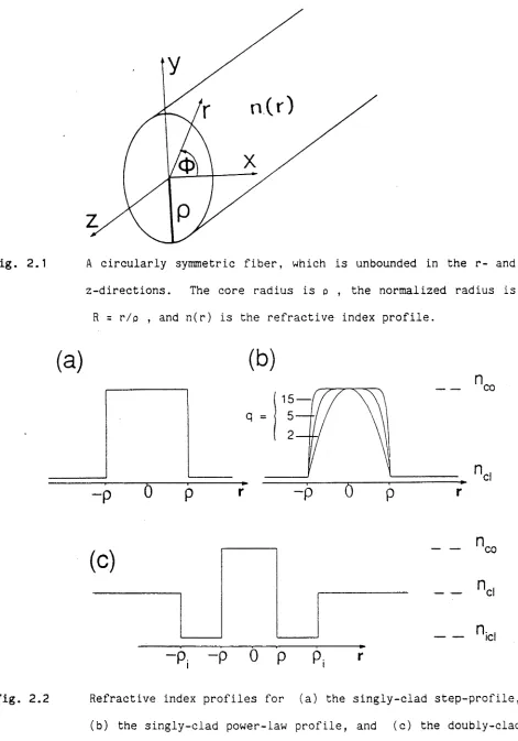
In figure 2.4 the cut-off values, V f are plotted against q. In figure 2.5(a) we plot the eigenvalue U against V for several values of q, and in figure 2.5(b) we plot U against q for several values of V.

q

Fig. 2.4 Cut-off values for the power-law profile against grading

- q=10

V

cut-off for LP mode

q

(c) Doubly-Clad Step-Profile Fiber

This profile is often called the W-fiber, or depressed inner- cladding fiber, and its profile is shown in figure 2.2(c). As we shall see in Chapter 3, this fiber has a shifted zero-dispersion wavelength [10,11], due to its multiple cladding, and can be used for minimum dispersion operation at longer wavelengths (and therefore less loss) than the singly-clad fibers. Following reference [11] we define two profile parameters

(2.27)

where n. is the refractive index of the inner cladding. We also define two V's according to eqn. (2.15)

1 / ? V = kon (2A) 17*

co

V. = kpn (2A.)1/2

l

cov

(2.2 8)

and the mode parameters are

U = o(k2n2o - 32

)1/2

(2.29)

We introduce the two main parameters

i

(2.30)

For the profile shape we have

f(R) =

l

, 0 < R < 1

, 1 < R < Q 1 , R > Q

The solution to equation (2.21) is then given by [11]

(2.32)

V T UR>

F *(R)

V j W . R ) + A2K,(W.R)

V i

0 < R < 1

1 < R < Q

R > Q

(2.33)

where I is the modified Bessel function of the first kind, and the A's are normalized constants which ensure the continuity of F (R) at the boundary R = 1 and R = Q. Analytic expressions for A's are presented in the Appendix. The eignevalue equation is found by matching the field and its first derivative at the boundaries R = 1 and R = Q:

[ y u) - y y l lywQ) + yw^)]

K

(U) + I

4

(W.)] [Ka(WQ) - ic^W.Q)]

Xl+1 V i

<V Ku i(¥>

(wiQ) V i (V

(2.34)

where

V x)

V x)

xV i (x)

(2.35)

V v) -

h {'

:) _

W 7*

V v

>

*

V 7

)

’

K1+,(

7

>

V,'7

Q

)

where V = V(-p^ J 17 ^ .

(

2

3 6

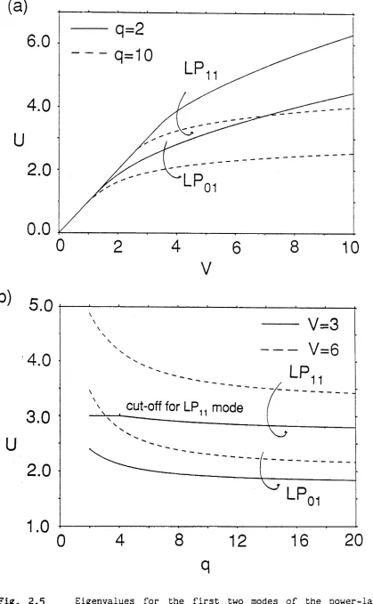
In figure 2.6 the cut-off curves are plotted against Q for several values of P. In figure 2.7(a) we plot the eigenvalue U against V for a fixed radius ratio Q and several values of profile ratio P, and in figure 2.7(b) we plot U against Q for several values of profile ratio and fixed V.

We mention here that variation of V for a given fiber implies variation of wavelength, and since refractive index is a function of X (see Chapter 3) then P must also be a function of X . However, in Chapter 3 we show that variation of P with respect to wavelength is very small, and throughout we regard P as constant.

P=0.25

-- P=0.50

Q

Fig. 2.6 Cut-off values for the W-fiber against radius ratio Q for

Q=1.5

P=0.25

- - P=0.50

P=0.5

cut-off for LPn mode

LP

Q

Fi.g 2.7 Eigenvalues for the first two modes of the doubly-clad

4. Polarization Corrections to the Step-Profile Fiber

In section 2-2(b) we saw that by using the "weakly-guiding", or A -*■ 0 , approximation the vector wave equation could be replaced by the scalar wave equation, and the fields can be described by plane waves which are called LP (linearly-polarized) modes.

An (a,m) mode will be designated as LP throughout this work, unless otherwise specified. We stress that LP modes are not the true modes of the fiber, they are only an approximation in which all polarization properties are ignored. However, we will show in later chapters that in fact the LP modes can be an accurate description of mode propagation if the fiber is perturbed in some manner.

In our study of birefringence in Chapter 6 we will have cause to use the vector properties of the modal field, so here we review the scheme in which vector fields are constructed from scalar fields, and consider a specific example. There are four solutions to the circularly-symmetric form of the scalar wave equation (2.19), which all have the same S's :

e = F (R) c o s H x

~xe l

e = F (R) cosiU y

-ye l ~

i = F„(R) sinib x

~xo l

(2.37)

i = F .(R) sinJU y

-yo l i

where F^(R) is the solution to eqn. (2.21).

Using symmetry methods these scalar solutions can be linearly

®1 e ~xe + e ~yo

e 2

S3 = 9 + e _~ye

(

2

38

e - e ~xo -ye

Mote that for the two fundamental ( l = 0) modes the exact: modes

are the same as the scalar modes. The correction to the propagation constant is now given by eqn. (2.14), with eu given by any one of eqn.

(2.38), and e, given by either of eqns. (2.37) that make u d e u .

As an example for determining the proper modes of a fiber, we consider the singly-clad step-profile fiber, whose scalar fields are given by eqn. (2.23). The scalar propagation constants are given by eqn.

(2.18a) :

3 = kn ( 1 - 2 4 — )1/2 (2.39)

CO V2

where use has been made of the definition of V, eqn. (2.15), and U is the eigenvalue of the scalar wave eqn. (2.21).

In order to evaluate eqn.(2.14) we use eqn.(2.17) and write Vtin n 2 » -2AVtf. Tor a step-profile f is a step-function at the boundary

R=1, and we can write

-2A V f = -2A 5(R-1) n (2.40)

A

where 5 is the Dirac delta function. The unit outward vector n is on the boundary interface in the waveguide cross-section. Furthermore

32 - 3 2 = 2s(ß - 3) = 2kn (3 §) =

-C0 (2A) o

where we have used the approximation eqn. (2.12). Eqn. (2.14) then reduces to

56 = o(2A) 3/2

2V \

(VSJ

5t’2 ds

1"

it-Sfc dA

K e r e ^ 5 = r^ a n <?f p r t L e/\< jln or> - f t a oour\cU <N j i r \ { £ ^ ^ c c

-In Table 2.1 we present the corrections to 3 for the four exact modes, where the modes are labelled in the standard EH and HE notation

(see (1] for a discussion). In figure 2.8 we plot the exact eigenvalue,

Uov against V for a fixed A = 0.01 . Uov is defined as

U 2 = o 2(k2n 2 - 3 2) = U 2 - 02(s2 - S 2) (2.43)

where U is the scalar eigenvalue given by eqn. (2.18a). Figure 2.8 thus represents the true modes propagating in a singly-clad step-index fiber, and should be compared to the approximate LP modes of figure 2.3. We note that the fundamental mode does not have a degeneracy split.

0

2

4

6

8

V

Fig. 2.8 The true modes in a singly-clad step-profile fiber. Uex is given by eqn. (2.43), and the modes are labelled by the HE and

Po

la

rization

c

o

rre

ct

ion

s

t

o

t

h

e

step-pr

of

ile

f

i

b

e

4. Gaussian Approximation to Modal Fields

The fundamental mode field of an optical fiber is approximately Gaussian in shape, and this fact can be exploited by giving very simple forms

for the modal parameters discussed in Section 2-3. The basis of the

approximation is that the fundamental mode of an arbitrary profile circularly symmetric fiber can be approximated by some Gaussian function:

where R 0 = rQ/p is called the spot-size. The problem then is to find an R 0 such that eqn. (2.44) gives a good approximation to the exact field. In this work we will only be concerned with approximations to step-profile fibers.

Marcuse [12] has determined the spot-size of the fundamental mode by minimizing the difference between the exact and Gaussian fields:

- -R2/2R2 F 0(R)

l^ ) - S

0 [ling--- '2 R d R

(2-45)

where M (R 0) and x 0 are normalization factors, with x 0 given by eqn. (2.25). The spot-size is then determined by

F 0(R) = exp(- R2/2R2) (2.44)

dl

0

o

For the step-profile fiber we have [12]

A second, variational, method for finding R Q is due to Snyder and Sammut [13].

This method has two advantages: first of all it results in a simple

expression for R 0 ; and secondly it can be generalized to describe higher- order modes [14].

The basis for the approximation is that the exact higher order modes of the infinite parabolic profile (i.e. f = R 2 in eqn. (2.21)) are given by

F (R) = ( f - ) 1 ( ^ ) e x p ( - R2/2R2)

1 0 * R2

(2.48)

R 2 = 1 / V . r U )

m-1 0

( l ) r R 21

m - 1 ^

m - 1

= Z

n

( - 1 ) ( m - 1 + O

n! (n+l)! (ra-1-n)! ( - ) n (2.49)

It is assumed that the modes of an arbitrary profile fiber are of the same form as eqn. (2.48). The spot-size is then chosen to minimize the variation in 3 when eqn (2.48) is substituted into a stationary expression for 3 . This expression can be obtained by multiplying the scalar wave equation (2.21) by

RF^(R) and integrating over the profile:

co d 2F . dF

U

= J

--

^ q-^lF2

o R 2 1 d R 2 ri an X/ o *

where U 2 is related to 3 2 by eqn. (2.18a). profile, the value of R Q is found by solving value of U [13]

Given f(R) for a particular

the equation for the extrem/um

(2.51)

2m + l V 2(m - 1)!

[ z+m- 1)! J 0 dR f — F 2 R2 dR I (2.52)

Given the solution of this equation for R 0 , the corresponding value of U, and

hence S , is found by substituting the extremum value of R 0 back into

eqn. (2.50).

For the step-profile fiber f(R) is given by eqn. (2.22), and the

derivative of f(R) is the Dirac delta function: df/dR = S(R-1) . For the

fundamental (z = 0, m = 1) mode eqn. (2.52) reduces to [13,14]

R 0 = (l/ZnV2)1/2 (2.53)

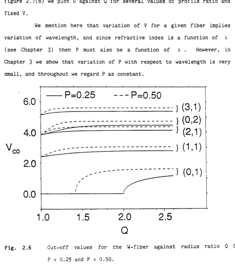
In figure 2.9 we compare eqns. (2.47) and (2.53). The two spot-

sizes behave similarly over a large range of V, although eqn. (2.53) will

break down as V + 1 . We discuss this later.

In Table 2.2 we list F (R), R 0 and U for the first two modes of the

step-profile fiber. The relative error of U with its exact value (i.e. the

eigenvalue equation (2.24)) is at most only a few percent [14].

Table 2.2: Gaussian Approximation for the Step-profile Fiber

Mode (z,m)

F * ( R ) Ro U 2

(0,1) 8 -R2/2R2 u u = e - 1/Ro (1 + J-)

- V2

(1,1) —R e-R2/2R2

2 1 -1/R2

— = — e 0 2 ( — + 1 * R ? )

°o _{V2 R 2}

eqn.(2.53)

1

2

3

4

5

6

V

Fig. 2.9 Comparison of spot-size definitions for the Gaussian approximation to the fundamental mode.

(1/R02).exp(-1/R02) - 2/V2

■ 1 i T ■ 3 ' ' t ' T r

0.0

0.5

1.0

1.5

2.0

R

2

no

In order to find R0 for the 2, > 1 modes one must use a zero finding method as outlined in the Appendix. In general the equation for RQ for these modes has more than one zero.

I

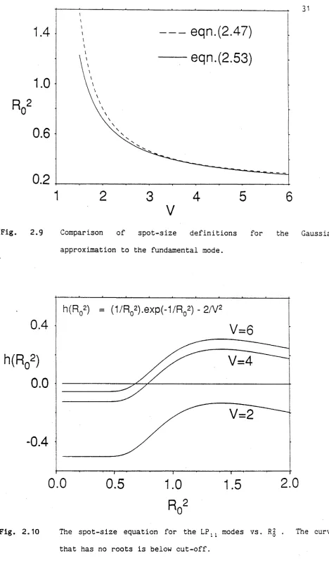
As an example for determining the spot-size for some mode we consider the LP, , mode (refer to Table 2.2), and in figure 2.10 we plot the function

h ( f ? o >

1 -1/R2 = — e 0

R 2

uo

2_ V 2

against R Q for several values of V. The curves that have no zero's are for V values below cut-off (for the step-profile fiber the L P l1 modes does not propagate for V < 2.405). The other curves may have multiple zero s, and in this case the correct value of R 0 (that value which gives the most accurate value of U) is given by the first zero.

In Table 2.2 R 0 is not the same for different modes, and we may

write

l , m

(V) = (2.54)

In figure. 2.11 we plot the function M against V for the first four modes. As mentioned previously, eqn.(2.53) will break down as V 1 . Henceforth, when using the Gaussian approximation to describe mode properties on single-mode fibers (i.e., those fibers with V < 2.4 ) we will use the spot-size given by eqn.(2.47). However, when we deal with the more general case of few-mode fibers we will use the spotsize defined by eqn.(2.52) for the

U , m ) mode, and represent this spot-size by ^ .

1.2

0.8

0.4

0.0

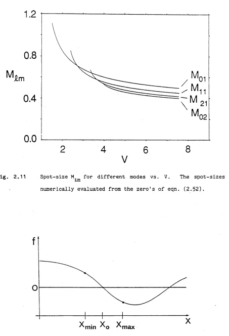
Fig. 2.11 Spot-size M for different modes vs. V. The spot-sizes are numerically evaluated from the zero's of eqn. (2.52).

max

m m

6. Aüpendix

(i) Zero finding routine for functions

To find the zero, x Q , of the function f(x) we write g = f(x) and

choose m i n i m u m and maximum values of x such that

"min < x, Xmax

as shown in fig. 2.12. We then determine x Q by the following routine: (with

reference to fig. 2.12)

ROUTINE ZERO ff, x . , x ; x j ^ ' min' m a x ’ 0J

start: x = 1/2 (x_._ + x

min ‘max

g = f(x)

is |g| < e , g < 0 , g > 0 ?

if g < 0 then x = x max

return to start

if g > 0 then x . = x

°

m m

return to start

if !g| < s then x Q = x

(2A.1)

e << 1 determines the accuracy of x. . x . and x can be found

J 0 m m max

automatically, and the routine can be generalized to find any zero of a

(ii) Eigenvalues and fields for arbitrary pofiles The differential equation for ehe core region is

y" + tl y

(u

v

o

R R 2

l2

(2A.2)

where f is the profile shape, eqn.(2.17). y must be continuous and have a continuous derivative y' at the fiber boundary R = 1, giving an eigenvalue equation for U:

Z_

y

2 KZ(W)

u)Kerc

(ieici m

C-Uciciiruj 15

(iij j

If we write equation (2A.2) in the form

y" = f(R,y,y') (2A.4)

then'for some value of V,f,z and U y and y' can be found at R = 1 by a fourth- order Runge-Kutta method

ROUTINE R-K( f,Z,V,U; y,y' )

For n=0,1...,N, d o :

y = y

K K

ya = ?(Rn ,ya ,y4)

yb = yn + 2 h y y ' = y' + t h y"

Jb n 2 a

y + - h y '

J n 2 J b ^ + 2 h yb

f(Rn - 2 h ’ yc ’yi

= y + hy' J d n J c

y' - y' + hy" d Jn w c

y" = f(«„ - h, yH , y,

(2A.5)

y

y

n + 1

n+1

= yn + ! u ; + 2yi + 2y; + y^

= yn + I (ya + 2yb + 2yc + yd^

Then y ^ and y^+ ^ are approximations to y and y ' , respectively, at

Rn+1 = R0 + • Usually we choose N = 1/h and h = 0.1. The intial conditions are

1 = 0: y 0 = 1

y'o =

0

y" = - U 2 + V 2f

1 > 1: y 0 = 0 (2A.6)

y'o --

1

y'o =

0

ROUTINE EIG (f,a,m,V,U . ,U ; U) min max

CALL ZERO ff(U); U . , U ; U)

v m m max '

where the function f(U) is the eigenvalue eqn. (2A.3)

f(U) = K 4 (W)y' + I W ( K ^ W - K l+1(W))y

and U and y,y' are given by

u = i (u . + a

)

2 v min m a xJ

CALL R-K(f,4,m,V,U; y,y')

(iii) Normalization constants for the W-fiber modal fields

The normalization constants of eqn. (2.33) are given by [11]

A 0 = 1/J4(U)

A, = ( W . J ^ U ) K1+1(W.) - a J 1+1(U) K j u . j j / J j u )

A, = ( H . J 4 (U) I 1+1(W.) + U J l + , ( 0 ) I J W . ) ) / J a (U)

A3 = ( A ^ J W . Q ) + A j K j W ^ J j / K ^ W Q )

(2A.7)

References to Chapter 2

[1] A.W. Snyder and J.D. Love, "Optical Waveguide Theory" (Chapman and Hall, Mew York, 1983)

[2] P. Lorrain and D. Corson, "Electromagnetic Fields and Waves" (W.H. Freeman, San Francisco, 1970)

[3] A.W. Snyder, "Asymptotic expressions for eigenfunctions and eigenvalues of a dielectric or optical waveguide"

IEEE Trans., MTT-17, pp. 1130-1138 (1969)

[4] D. Gloge, "Weakly-guiding fibers"

Applied Optics, ±0, pp. 2252-2258 (1971)

[5] J.A. Arnaud, "Transverse coupling in fibre optics part II" Bell. Syst. Tech. J., 53, pp. 675-696 (1974)

See Appendix

[6] C.M. Kurtz, "Scalar and vector mode relations in gradient index light

guides"

J. Opt. Soc. Am., 65, pp. 1235-1240 (1975)

[8] D.L.A. Tjaden, "First-order correction to weak guidance approximation in fibre optics theory"

Phillips J. Res., 33, pp. 103-112 (1978)

[9] D. Gloge and E.A.J. Marcauiii, "Multimode theory of graded-core fibers" Bell. Syst. Tech. J., 52, pp. 1563-1578 (1973)

[10] S. Kawakami and S. Nishida, "Perturbation theory of a doubly clad optical fiber with a low index inner cladding"

IEEE J. Quantum Electron., QE-11, pp. 130-138 (1975)

[11] M. Monerie, "Propagation in doubly clad single-mode fibers" IEEE J. Quantum Electron., QE-18, pp. 535-542 (1982)

[12] D. Marcuse, "Loss analysis of single-mode fiber splices" Bell. Syst. Tech. J., 56, pp. 703-718 (1977)

[13] A.W. Snyder and R.A. Sammut, "Fundamental (HE 11) modes of graded optical fibers"

J. Opt. Soc. Am., 69, pp. 1663-1671 (1979)

[14] J.D. Love and C.D. Hussey, "Variational approximations for higher-order

modes of weakly guiding fibres"

Opt. Quantum Electron., J_6, pp. 41-48 ( 1984)

u

[15] M. Abramowitz and I.A. Stegen, " (Dover, Hew York, 1964).

CHAPTER 3

DISPERSION OF LIGHT IN GLASS OPTICAL WAVEGUIDES

1. I n t r o d u c t i o n

2. T he D i s p e r s i o n R e l a t i o n s

3. M a t e r i a l D i s p e r s i o n

4. W a v e g u i d e D i s p e r s i o n

5. M odal G r o u p D elay

6. T he Z e r o - D i s p e r s i o n W a v e l e n g t h

(a) S i n g l y - C l a d F i b e r s

(b) D o u b l y - C l a d F i b e r s

7. S i n g l e - M o d e F i b e r s O p e r a t i n g at F e w - M o d e W a v e l e n g t h s

3. A p p e n d i x

(i) P r a c t i c a l u n i t s for

(ii) C o m p a r i s o n o f ex a c t

d i s p e r s i o n

CHAPTER 3

DISPERSION OF LIGHT IN GLASS OPTICAL WAVEGUIDES

1. Introduction

In Chapter 5 we will see that phase-matching the stimulated four-photon mixing process is very sensitive to the dispersion properties of the fiber, and an understanding of such properties is essential to explain experimental results which are presented in later Chapters. As well, dispersion effects are the key to the optimum use of practical fiber systems. In this Chapter we present results which will be referred to throughout this work, as well as some results which are of interest for various optical fiber applications.

Dispersion is one of the detrimental factors inherent to light propagation in optical fibers. When a pulse of light propagates along a waveguide several dispersion effects contribute to distort its shape.

Normally material dispersion dominates, but in the region X = 1.3 uni (where the fiber is usually single-moded) material dispersion is -zoee- and the waveguide dispersion controls the total dispersion.

Inter-modal dispersion is due to the fact that the modes of an optical fiber propagate with different group velocities, so another dispersive effect is the difference in the group delay between modes. Thus if a pulse is formed by more than one mode it will spread out as it propagates along the fiber. As we shall see in Chapter 5 this inter-modal dispersion effect is the key to phase-matching the stimulated four-photon mixing process in few-mode fibers. This form of dispersion can easily be eliminated by having only one mode propagate - this is why single-mode fibers are the most commonly used for fiber communication systems. None the less, even a few mode fiber can be optimized to reduce this dispersion, as we show later. In figure 3.1 we schematically represent

intra- and inter-modal dispersion.

After presenting the dispersion relations we investigate the change in refractive index with respect to wavelength. We are only concerned with fibers that have a refractive index in-the-cladding that is pure silica, and the -refraotive— ind»x— in— core is Ge02-doped silica. We show the variation of refractive index, material dispersion and profile height with respect to wavelength for several amounts of Ge0o dopant, and show that there is a linear relation between refractive index and the

amount of GeO., for any wavelength.

range, where the loss is much lower. We consider some examples of this shifting effect and present numerical results.

As an example of dispersive effects in optical waveguides, we examine the case of a singly-clad step-index fiber designed for single­ mode operation at a wavelength of 1.3um that is then used in the few-mode range of 0.85um . This is a problem of practical interest, because most single-mode fibers currently being manufactured are designed to achieve optimum performance at X = 1.3 um , but the most inexpensive sources operate at the lower wavelength. In applications such as local area networks, where transmission is required over relatively short distances and large numbers of sources and detectors may be used, the combination of readily available fibers designed for 1.3 uni and sources operating at 0.85 urn is desirable, provided that adequate performance can be achieved. (See mf. {-on (K d i s c U S S i o f live jf

Sys + em local .

loe

concerned-8

t = intra-modal dispersion

dispersion properly m

^»3

discussion.')

5T = inter-modal dispersion

5T = T, - T

mode 1

mode 2

transit time

2. The Dispersion Relations

The scalar propagation constant is given by eqn. (2.39).

Because we are using the weakly-guiding approximation, so that A << 1 , we may write

kn (1 - A — )

p n v '

G O y 2 (3.1)

We define the dimensionless group delay as dß r _ dn U dU r,_ dA

as r . an u au r .

— = (n + k — — Tr — Ikn —

r\ir L dk V dV ^ Alr

(3.2)

where we have set n = nCQ for simplicity. The conversion of eqn. (3.2) to practical units is given in the Appendix.

As we shall see later, we can neglect terms of order

A(k/n)(dn/dk) and (dA/dk) and write the group delay for each mode as

t = N + nAT _(3.3)

where

N = N (A ) = n + k ~~ = n(\) ak

dn( A ) dA

is the group index and

T e T(V) U2

\J2

U dU V dV

(3.4)

(3.5)

The intra-modal dispersion, or total dispersion, of a mode is the spread in the group delay due to the small spread in wavelength of the source of transmission, and here we define it as

St = (t/x) sx (3.6a)

t

t

c

421

D( X ) dT

+ nAV dV

(3.6b)

where

D(X) = 2k

4a

dk2 dX2

is the material dispersion of the bulk material from which the fiber is made, and V(dT/dV) is the waveguide dispersion, and depends only on the geometry of the guide. The total dispersion can then be expressed as a combination of material and waveguide dispersions:

t = t +

m nA tw (3.8)

3. Material Dispersion

In this section we will investigate the variation of the refractive index, profile height, and material dispersion with respect to wavelength. Throughout this thesis we consider an optical fiber in which the refractive index of the cladding, n , is composed of pure silica, and the refractive index of the core, nQ 0 , is composed of GeO, doped silica. We find that there is a linear relation between nCQ and the amount (molar percent, m) of GeO, for any given wavelength. Throughout this work we will be mainly concerned with the wavelength range

0.5 um < X < 1.5 urn .

The experimental variation of refractive index with wavelength can be fitted to a three term Selimeir dispersion relation of the form

where are constants related to material oscillator strengths and i. are the oscillator wavelengths. The dispersion can then be found by direct differentiation:

(3.9)

n is 1 3? \3

(3.10a)

i

d X 2 n i = 1 33 \ 6 i =i= 1 3? X 1* n is 1 3? X 3

l i i

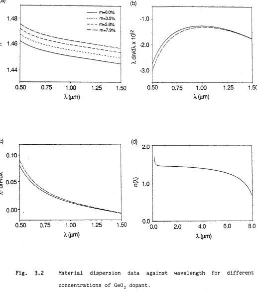
We use the experimental results of reference [4], in which the values of A^ and 2, are determined for 5 different amounts of Ge02 , including the pure silica case. We define the quantity m to be the molar percent of G e 0 2 dopant in the core, and consider m = 0%, 3.1*, 5.8$ and

1

9

In figure 3.2 we use eqns.(3.9) and (3.10) and plot a) n(x), b) X dn/dX and c) X 2 dn/dX2 against wavelength for the different m. In fig. 3.2(d) we plot n, against X over a large range of wavelengths and find that the Sellmeir equation (3.9) breaks down for X < 0.3 and X 1 8.0 . We note that material dispersion (eqn.(3.7)) is zero at around X = 1.3 um .

As mentioned previously, we consider fibers in which the cladding is considered to be pure silica (0 GeO, ). Thus the profile height is directly related to the amount of dopant in the core. In fig. 3.3 we plot a) A and b) x dA/dX against wavelength for different amounts of G e 0 2 in the core. We note that fig. 3.2(b) and fig. 3.3(b) justify our approximation of eqn. (3-3) where terms of order

A(k/n)(dn/dk) and k(dA/dk) are neglected.

--- m-O.0% --- m=3.5% --- m«S.8% --- m=*7.9%

c 1.46

A.(jum)

A. (jam)

zx

n

x

v

(a)

1.0

0.0

f

---L __ _

2.0

n \

Ö t

$ 1-0'

m=3.5%----nd : : m*5.8%---- _0.0

m=7.9%---0.50 0.75

Fig. 3.3

1.00

A. (urn)

\ \

\ \

\ \

\ \

-1.25 1.50 0.50 0.75 1.00

X(jim )

1.25 1.50

Profile height against wavelength. The cladding is assumed pure silica (m = 0% ) and the core has different concentrations of

Ge02 dopant.

n(X,m) = n(x,0) + {n(X,7.9) - n(X,0)} m/7.9 (3.11a)

D (X ,m ) = D(X,0) + {DC X ,7.9) - D(X,0)} m/7.9 (3.11b)

and hence

A ( X , m ) = ~ {1 - n- (-U ° I } . (3.11c) n 2(X,m)

Equations (3*11) are the basis for evaluating the theoretical

results on four-photon mixing and mode propagation that will be presented

later. In the Appendix we express our dimensionless dispersion D(X) in

practical units.

4. Waveguide Dispersion

We are interested in the waveguide part of the intra-modal

dispersion relation (3.8):

? tJ dUx

V d V J (3.12)

For the singly clad step-profile fiber one can differentiate the

Z . 2.1»*

eigenvalue equation (-g —19) with respect to V to obtain

K2(W)

:

Vi(H) K

1

+i(w)}

t

w 2 — { ( 1 -2< ) < + — (1 - — (1 - <)) x

V2 W 2 V2

WK (W) WK (W)

^Ka+1(w) +

“ 7T

)^1<

^ + 2<^'

where

(3.14)

K*(W)

K = :

V l (W)

For the fundamental mode (i=0) eqn. (3-14) reduces to the result of

reference [6]. Usually, only the waveguide dispersion of the fundamental mode is important, because in few-mode fibers the inter-modal and material

r

disp^sion will dominate.

For the clad power-law profile and W-fiber the waveguide

dispersion t is evaluated numerically, with eigenvalue U specified in

Section 2-3. In fig. 3.5(a) the fundamental mode waveguide dispersion t is plotted against V for the clad power-law profile with several values of profile parameter q. ( q = « is the step-profile, given by eqn. (3.14)), and in fig. 3.5(b) we plot t against q for a fixed value of V = 2.2.

In Section 3-6 we examine the intra-modal dispersion in the wavelength region where tm is very small, so that t plays a major role in determing the zero-dispersion wavelength.

2

---0

1

2

3

V=2.2

q

P=0.5

2 .0

----0

1

2

3

V=2.2

0.50 H

P=0.25

— P=0.50

0.00J

Q

Fig. 3.6 Waveguide dispersion of the fundamental mode for the W-fiber. (a) t vs. V for a fixed P and different radius ratio Q; and

w

(b) tfI vs. Q for a fixed V = 2.2 and several values of P.

5. Modal Group delay

We now consider the few mode case dispersion is the major cause of pulse spreading, is the difference in group delays of the modes, fiber the modal group delay is

in which inter-modal Inter-modal dispersion For the step-profile

T im

U2

V2

{-Kjj(W)

Vl(W)

- 1) (3.15)

where we have substituted eqn. (3.13) into eqn. (3.5). For the clad power-law profile and W-fiber eqn. (3.5) is evaluated numerically.

In figure 3.7 we plot T for the first five modes against normalized frequency V. Figure 3.8(a) is a plot of T against V for the clad-power law profile for several values of q, and fig. 3.8(b) is a plot of T against q for several values of V.

In figure 3.9 we consider the W-fiber, and in (a) we plot T against V for a fixed Q and several values of P, while in (b) we plot T against Q for fixed P and several values of V.

0

2

4

6

8

V

(b)

— V=6

q

Fig. 3.8 Modal group delay for the clad power-law profile. (a) T vs. V

Q=1.5

P=0.25

- - P=0.50

P=0.5

--- V=6

Q

6. The Zero-Dispersion Wavelength

In Chapter 5 we will see that phase-matching the stimulated four-photon mixing process on single mode fibers depends critically on the zero-dispersion wavelength. In this Section we review the concepts and basic design considerations for achieving zero-dispersion operation on optical fibers.

In Sections 3-3 and 3-4 we looked at material and waveguide dispersion seperately. In this section we examine the total intra-modal dispersion (i.e. eqn. (3.6)) for a single mode fiber in the region where material dispersion t is small and the dominant effect is the waveguide dispersion. We consider some specific examples.

In figure 3.10 we give a typical loss curve for a Germanium doped core optical fiber. The peak at X = 1.4 urn is due to •water OH ions. Thus a fundamental design principle is to operate at longer wavelengths to reduce losses, but avoid the OH peaks. 1.3 um and 1.55 um are ideal operating wavelengths.

OH peak

scattering loss

As shown in fig. 3.2(c) material dispersion is zero near 1.3um , and waveguide dispersion will dictate at which wavelength the total dispersion is zero. When using optical fibers we want minimum loss and dispersion, so one muse design a fiber that will have zero dispersion at either 1.3 urn or 1.55 urn .

(a) Singly-Clad Fibers

We require total dispersion, eqn. (3.6), to be zero at some specified wavelength X so that

zd 3"(V ) = 0 , where the prime means differentiation with respect to k, and V contains all material and waveguide information. We now consider only the clad power-law profile.

If we specify the molar percent of Ge02 in the core, m, and the wavelength at which total zero-dispersion is wanted, then the only waveguide variables will be profile shape, q, and core radius, p :

5 " 0 . * z d ; q,ezd ) = o (3.16)

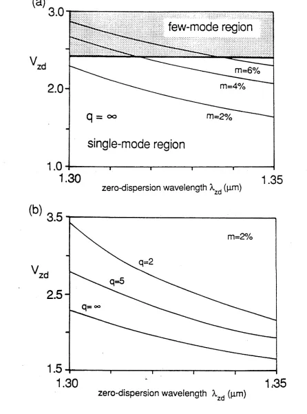
If q is specified, then o^ , which is the core radius at which 3" = 0 , can be determined by the numerical zero-finding procedure outlined in the Appendix of Chapter 2. Vzd= v(m,X ^,p is then also determined.

In fig. 3.11(a) we consider a step-profile fiber and show the variation of with respect to zero-dispersion wavelength X ^ , for several concentration of Ge0o dopant. (m and X ^ specify nCQ and A , and eon (3.16) then gives 0 , and hence V , ). The fiber is multimoded in the

zd zd

shaded region. In fig. 3.11(b) we show variation of V ^ with X ^ for a

few-mode region

single-mode region

zero-dispersion wavelength

Xz0

(jim)

zero-dispersion wavelength

Xzd

(jim)

F i g . 3 . 1 1 The V value, V^d , for which a clad power-law profile has zero

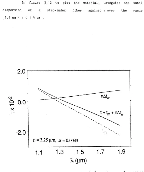
In figure 3.12 we plot the material, waveguide and total dispersion of a step-index fiber against X over the range

1.1 um < X < 1.9 um .

p = 3.25(im, A = 0.0045

X (|im)

Fig. 3.12 The material, waveguide and total dispersion, t, of a step-index fiber with parameters p = 3.25 um and A = 0.0045 . The dotted line is the numerical derivative k d 2S/dk2 , demonstrating the