Production function analysis of small rubber farms in Sri Lanka

OF SMALL RUBBER FARMS IN SRI LANKA

by

TEO CHOO-KIAN

A dissertation submitted in partial fulfilment of the requirements for the degree of Master of Agricultural Development Economics in the

Australian National University

D E C L A R A T I O N

Except where otherwise indicated, this dissertation is my own wo r k .

A C K N O W L E D G E M E N T S

I am extremely grateful to the Malaysian Government for granting me the opportunity of studying at the Australian National University (ANU) and to the Government of Australia for providing the Colombo Plan

Scholarship.

I wish to express my sincere gratitude to Dr R. Gregory of the Department of Economics, Research School of Social Studies, ANU, for his supervision, guidance and critical comments of the draft of the disser­ tation.

In particular, my special thanks are due to Dr C. Barlow of the Department of Economics, Research School of Pacific Studies, ANU, and to Dr D. Etherington and Dr M. Saad, both of the Masters Programme in the Economics of Agricultural Development, Development Studies Centre, ANU, for their every help, inspiration and encouragement throughout my

study period at the ANU.

I am also grateful to Mr M. Ray, Mrs G. Robbins, Mrs A. Sandilands of the Computer Services Section, Research School of Pacific Studies/ Social Studies, ANU, for their help in computer programming problems. My special thanks also goes to the Rubber Research Institute of Sri Lanka for granting me permission for the use of the survey data.

I am indebted to Miss M. Hewlett and Miss R. Kruger for typing the draft of this dissertation, and to Mrs P. Lyall for typing the final copy.

A B S T R A C T

The main purpose of this study has been to estimate the Cobb- Douglas production function from the cross-section input-output data of small rubber farms in the Agalawatta district of Sri Lanka. Twelve factors of production believed to affect output of rubber were identi­ fied, out of which four factors, namely, planting density, farm size, tapping frequency, and tapping age of the trees were considered in the estimating equation. The function was estimated for clone PB86 and clone Tjir 1 separately; and for each clone, the Cobb-Douglas function was estimated by two different techniques, namely, the Ordinary Least

Squares method which estimates the average function, and the Linear Programming method which estimates the best or the frontier function.

As a first step in the analysis, simple correlation and simple regression methods were employed with a view to bringing out relation­ ships between each of the specific factors and the output per acre. Next, the relationship between the four factors of production and the output of rubber was examined within the framework of multiple

regression analysis.

The estimated coefficients were used to predict output per acre for each clone. For both clones, the results strongly suggested that for every farm or group of farms for every year or group of years, there is a separate yield curve. Instead of a single production function, there exists a family of functions depicting various efficiency levels.

V e c t o r s o f t e c h n i c a l e f f i c i e n c y r e l a t i v e t o t h e a v e r a g e and

r e l a t i v e t o t h e f r o n t i e r w e r e g e n e r a t e d . The r e s u l t s showed t h a t t h e r e

e x i s t e d a w i d e r a n g e o f t e c h n i c a l e f f i c i e n c y a t f a r m l e v e l . T h i s b i g

d i f f e r e n c e i n e f f i c i e n c y c o u l d b e due t o s o i l q u a l i t y , m a na g em en t , o r

e v en b e due t o e r r o r s o f m e a s u r e m e n t i n t h e v a r i a b l e s u s e d f o r t h e

p r o d u c t i o n f u n c t i o n a n a l y s i s . I t i s c l e a r t h a t f u r t h e r r e s e a r c h i s

n e e d e d t o c l a r i f y t h e t r u e m e a n i n g o f t h e s e " e f f i c i e n c y " i n d i c e s a s

a p p l i e d t o t h e r u b b e r s m a l l h o l d e r s .

When t h e e f f i c i e n c y r a t i n g s f rom t h e a v e r a g e and t h e f r o n t i e r

f u n c t i o n s w e r e c o m p a r e d , i t was f o u n d t h a t t h e r a n k i n g o f t h e f a r m s w e r e

s i m i l a r i r r e s p e c t i v e o f w h e t h e r t h e r a t i n g s w e r e c a l c u l a t e d r e l a t i v e t o

t h e a v e r a g e o r t o t h e f r o n t i e r f u n c t i o n .

M a r g i n a l r e t u r n s t o f a c t o r s o f p r o d u c t i o n f o r i n d i v i d u a l f a r m s

r e v e a l e d t h a t t h e r e was no s i g n i f i c a n t r e l a t i o n s h i p b e t w e e n f a r m s i z e

and t h e m a r g i n a l r e t u r n s t o t h e l a n d . Unde r t h e a s s u m p t i o n o f p e r f e c t

m a r k e t s , and a s s u m i n g t h a t t h e p r i c e o f r u b b e r was Rs. 1 . 0 0 p e r po und

and t h e a v e r a g e wage r a t e was R s . 5 . 0 0 p e r d a y , i t was f o u n d t h a t f o r

PB86 f a r m s , t h e m a j o r i t y o f t h e s m a l l e r f a r m s h a d o v e r u s e d t h e t a p p i n g

l a b o u r , and n e a r l y a l l t h e l a r g e r f ar ms h a d u n d e r u t i l i z e d t h i s i n p u t ;

f o r T j i r 1 f a r m s , a l l t h e s m a l l e r f a r ms and a b o u t 50 p e r c e n t o f t h e

l a r g e r f a r m s h a d o v e r u s e d t h e t a p p i n g l a b o u r , a n d u n d e r u t i l i z a t i o n o f

t a p p i n g l a b o u r o c c u r r e d o n l y i n t h e l a r g e r f a r m s . U n d e r u t i l i z a t i o n o f

l a b o u r i n l a r g e r f a r m s , w h i c h w e r e t h o u g h t t o b e h e l d by a b s e n t e e

l a n d l o r d s , c o u l d b e due t o a s h o r t a g e o f l a b o u r o r an u n a t t r a c t i v e

n a t u r e o f t h e s h a r e - a r r a n g e m e n t o r t h e w a g e - p a y m e n t .

S i n c e t h e r e w e r e s u b s t a n t i a l amo u nt s o f n o n - r u b b e r c r o p s s u c h a s

p a d d y , c o c o n u t and t e a i n t h e a r e a , i t may h a v e b e e n a m i s t a k e t o i g n o r e

t h e s e c r o p s i n an e c o n o m i c s u r v e y and t o o b t a i n i n f o r m a t i o n r e l a t i n g

o n l y t o r u b b e r . H e n c e , g r e a t c a u t i o n i s n e e d e d when u s i n g t h e a n a l y s i s

f rom s u c h a s u r v e y t o g i v e any c r o p - s p e c i f i c a d v i c e b e c a u s e t h e i n f o r ­

ACKNOWLEDGEMENTS ... ABSTRACT ... LIST OF TABLES ... LIST OF FIGURES ...

k k -k

CHAPTER

1 INTRODUCTION ... . 1.1 Objectives of This Study ... 1.2 Nature of the Data and

Limitation of the Study

1.3 Brief Notes on the Importance

of Rubber in Sri Lanka ... 1.4 The General Setting ...

1.4.1 The Physiography of the Area 1.4.2 The Farm Structure

1.4.3 Sampling Procedure

1.4.4 Samples for the Present Study

Page (iii) (iv) (x) (xii)

1 1

2

2

6

6 6 7

8

2 AVERAGE AND FRONTIER PRODUCTION FUNCTIONS: THEORETICAL CONSIDERATIONS ... 2.1 The Production Functions ... 2.2 Properties of the Cobb-Douglas Function .. 2.3 Ordinary Least Squares Procedure

2.4 Frontier Production Function 2.4.1 Method of Estimation

Estimation of Technical Efficiency ..

Contents (continued)

-CHAPTER 3

4

RUBBER CULTIVATION AND FACTORS AFFECTING RUBBER PRODUCTION ... 3.1 Cultivation of Rubber

3.1.1 Planting Materials

3.1.2 Exploitation of Rubber Trees 3.1.3 Commercial Rubber Sheets

Page

21 21 24 25 28 3.2 Factors Affecting Rubber Production 29

3.2.1 Annual Inputs controlled by

the Smallholder 30

3.2.1.1 Labour Input in Tapping

Rubber Trees .. .. .. 30 3.2.1.2 Supplementary Inputs .. 31 3.2.1.3 Management Factor . . . . 32 3.2.1.4 Types of Cut in Tapping

Rubber Trees .. .. .. 34 3.2.2 Lagged Values of the Inputs

Applied in Previous Years _{• •} 34

3.2.2.1 Planting Density 34

3.2.2.2 Size of the Farm 35

3.2.2.3 Age of the Trees 35

3.2.2.4 Clone or Variety

of Rubber . . 36

3.2.2.5 Distance of the

Holding ... . . 36 3.2.3 Completely Exogenous Variables 36

SPECIFICATION OF THE VARIABLES AND THE ANALYSIS OF SPECIFIC FACTORS AFFECTING

OUTPUT ... 38

4.1 Specification of the Variables 38

4.1.1 Output ... 39

C o n t e n t s ( c o n t i n u e d )

-CHAPTER

4 . 1 . 3 T a p p i n g F r e q u e n c y . . 4 . 1 . 4 F a r m S i z e

4 . 1 . 5 T a p p i n g Age o f t h e T r e e s 4 . 1 . 6 M a n a g e me n t

4 . 2 A n a l y s i s o f t h e S p e c i f i c F a c t o r s A f f e c t i n g O u t p u t

4 . 2 . 1 B i v a r i a t e A n a l y s i s

4 . 2 . 1 . 1 A f f e c t o f e a c h S e l e c t e d V a r i a b l e on Y i e l d

4 . 2 . 1 . 1 . 1 Y i e l d p e r A c r e b y Age

4 . 2 . 1 . 1 . 2 Y i e l d p e r A c r e b y P l a n t i n g D e n s i t y . . 4 . 2 . 1 . 1 . 3 Y i e l d p e r A c r e

b y T a p p i n g F r e q u e n c y

4 . 2 . 1 . 1 . 4 Y i e l d p e r A c r e b y F a r m S i z e . . 4 . 2 . 1 . 2 Summary

5 EMPIRICAL PRODUCTION FUNCTION ... 5 . 1 M o d i f i e d Form o f C o b b - D o u g l a s F u n c t i o n 5 . 2 T e s t f o r S i g n i f i c a n t D i f f e r e n c e s

i n C l o n e E f f e c t

5 . 2 . 1 R e s u l t s o f t h e Chow T e s t

5 . 3 M u l t i c o l l i n e a r i t y ... 5 . 4 A v e r a g e P r o d u c t i o n F u n c t i o n :

E s t i m a t e d C o e f f i c i e n t s a n d t h e

R e l a t e d S t a t i s t i c s ... 5 . 4 . 1 P r o d u c t i o n E l a s t i c i t i e s

5 . 4 . 1 . 1 P r o d u c t i o n E l a s t i c i t y o f T a p p i n g F r e q u e n c y

P a g e 40 42 42 42

43 46

50

50

57

61

66

70

72 72

74 76 80

80 81

Contents (continued)

-CHAPTER Page

5.4.1.2 Production Elasticity

of Planting Density .. 82 5.4.1.3 Production Elasticity

of Farm Size .. .. .. 85 5.4.1.4 Production Elasticities

of Age Factors . . . . 85 5.5 Frontier Production Function .. .. .. 96

6 TECHNICAL EFFICIENCY AND MARGINAL

PRODUCTIVITY ... 100

6.1 Technical Efficiency 100

6.1.1 Comparison of the Efficiency Ratings from the Average and the Frontier Production

Functions .. .. .. .. .. 102 6.2 Marginal Returns to Factors of

Production .. .. .. .. .. .. 103

7 SUMMARY AND C O N C L U S I O N S ... 119

•k k k

BIBLIOGRAPHY ... 124

k k k

APPENDIX TABLE I: TECHNICAL EFFICIENCY RATINGS

AND R A N K I N G ... 127

APPENDIX TABLE II: MARGINAL PRODUCTIVITIES OF INPUT FACTORS BY INDIVIDUAL

FARMS ... 135

Table 1.1

1.2

1.3 1.4 1.5 3.1

4.1

4.2a

4.2b

4.3

4.4

4.5

4.6

5.1

5.2a

5.2b

5.3 5.4a

L I S T O F T A B L E S

Title Page

Composition of Exports of Sri Lanka,

1969-73 3

Area under Rubber Cultivation by size of

Holdings .. .. .. .. .. .. .. 4

Annual Export of Rubber from Sri Lanka .. 5 Crop Acreage and Number of Holdings .. 7 Number of Observations by Age . . . 9 Weight of Scrap as a Percentage of the

Weight of Rubber Sheets . . . 26 Summary of the Analysis of Variance:

Mean Yield by Clone .. .. .. .. .. 45 Simple Correlation Coefficients between

Yield and the Selected Variables:

PB86 Farms ... 48 Simple Correlation Coefficients between

Selected Variables: Tjir 1 Farms . . . . 48 Summary of the Analysis of Variance:

Yield per Acre by Tapping Age .. Summary of the Analysis of Variance: Yield per Acre by Planting Density .. Summary of the Analysis of Variance: Yield per Acre by Tapping Frequency Summary of the Analysis of Variance: Yield per Acre by Farm Size

Summary of the Estimated Coefficients

and the Related Statistics . . . 77 Simple Correlation Coefficients between

Selected Variables of PB86 . . . 28 Simple Correlation Coefficients between

Selected Variables of Tjir 1 .. .. 29 Predicted Yield in lbs per Acre of RSS .. 86 Mean of Planting Density and Tapping

Frequency according to Tapping Age:

Clone: PB86 ... 94 52

58

63

List of Tables (continued)

-Table Title Page

5.4b Mean of Planting Density and Tapping

Frequency according to Tapping Age:

Clone: Tjir 1 .. .. .. .. .. 95

5.5 Coefficients of Production Functions

Estimated by Ordinary Least Squares

and Linear Programming Methods . . . . 97

6.1a Geometric Means, Production Elasticities

and Marginal Productivities of Selected Inputs for Different Ages, Rubber

Clone: PB86 ... 106

6.1b Geometric Means, Production Elasticities

and Marginal Productivities of Selected Inputs for Different Ages, Rubber

Clone: Tjir 1 ... 107

Figure 1.1 1.2 2.1 4.1 4.2A

4.2B

4.3A 4.3B 4.4A

4.4B

4.5A

4.5B

4.6A 4.6B 5.1

5.2

5.3A

5.3B

5.3C

L I S T O F F I G U R E S

Title Page

Main Rubber-growing Areas of Sri Lanka .. (xiv) Area where Survey was carried out .. .. (xv) Technical and Price Efficiency . . . . 16 The Effect of Management Bias . . . 44 Frequency Distribution of PB86 Farms:

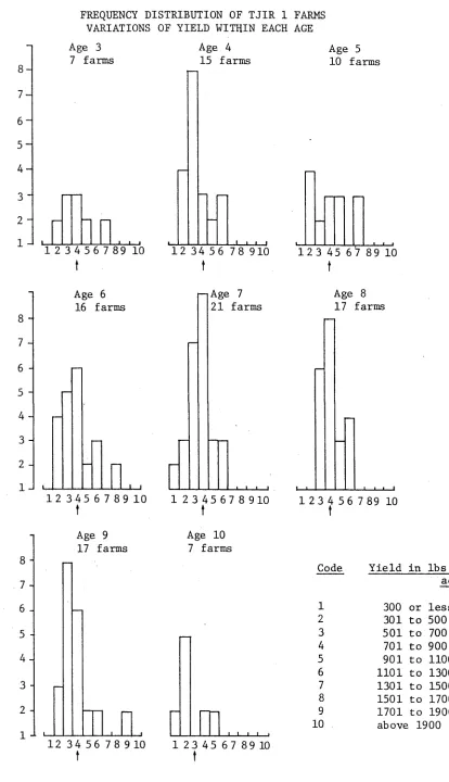
Variations of Yield within each Age .. 53 Frequency Distribution of Tj'ir 1 Farms:

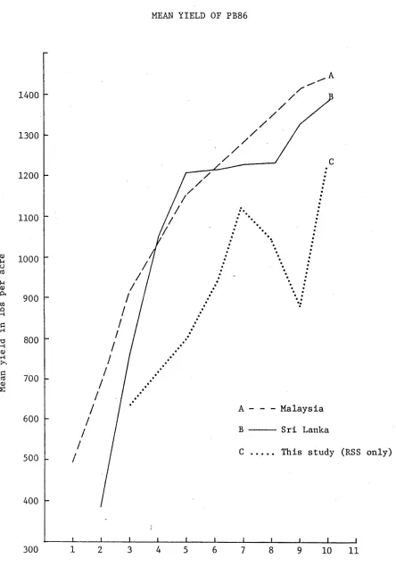
Variations of Yield within each Age .. 54 Mean Yield of PB86 .. .. .. .. . . 55 Mean Yield of Tjir 1 ... 56 Yield per Acre by Planting Density:

Clone PB86 ... 59 Yield per Acre by Planting Density:

Clone Tjir 1 ... 60 Yield per Acre by Tapping Frequency:

Clone PB86 64

Yield per Acre by Tapping Frequency:

Clone Tjir 1 65

Yield per Acre by Farm Size: Clone PB86 68 Yield per Acre by Farm Size: Clone Tjir 1 69

Effect of Tapping Frequency on Yield with

other Input Levels held Constant . . . . 83 Effect of Planting Density on Yield with

other Input Levels held Constant . . . . 84 Alternative Interpretation of Rubber Yield

and their Paths over Time.

Clone: PB86 (budgrafted) .. .. .. .. 88 Alternative Interpretation of Rubber Yield

and their Paths over Time.

Clone: PB86 (budgrafted) . . . 89 Alternative Interpretation of Rubber Yield

and their Paths over time.

List of Figures (continued)

-Figure Title Page

5.4A Alternative Interpretation of Rubber Yield

and their Paths over Time.

Clone: Tjir 1 (C.S.) ... 91

5.4B Alternative Interpretation of Rubber Yield

and their Paths over Time.

Clone: Tjir 1 (C.S.) ... 92

5.4C Alternative Interpretation of Rubber Yield

and their Paths over Time.

Clone: Tjir 1 (C.S.) ... 93

6.1A Efficiency Ratings of Clone PB86 Farms .. 104

6.IB Efficiency Ratings of Clone Tjir 1 Farms 105

6.2A Clone PB86: Marginal Productivity .. .. Ill

6.2B Clone Tjir 1: Marginal Productivity .. 112

6.3A Marginal Productivity of Land in Relation

to Area: Clone PB86 .. .. .. .. 113

6.3B Marginal Productivity of Land in Relation

to Area: Clone Tjir 1

6.4A Marginal Value Product of Tapping Days in

Relation to Area: Clone PB86 ..

6.5A Marginal Value Product of Tapping Days in

Relation to Area: Clone Tjir 1 .. .. 116

114

115

FIGURE 1.1

MAIN RUBBER-GROWING AREAS OF SRI LANKA

O Survey " ^ 3 Rubber

A n n u a l rai nf al l (millimetres)

FIGURE 1.2

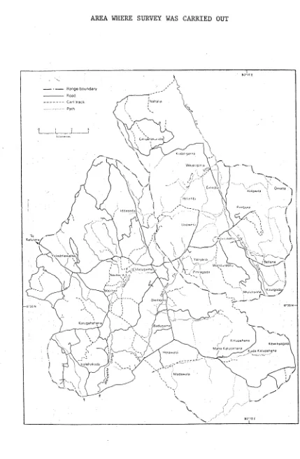
AREA WHERE SURVEY WAS CARRIED OUT

INTRODUCTION

1.1 Objectives of This Study

This study is an attempt to derive a production function for smallholder rubber of the Agalawatta District in Sri Lanka. There is extensive literature relating to the estimation of production functions; for example, Heady and Dillon (1961), Paris (1966), Timmer (1970) and Muller (1974), just to name a few. However, literature on the estimation

of production functions for perennial crops in peasant agriculture is still very limited. One such example is the study by Etherington (1973) on smallholder tea in Kenya.

There is a wide variation in output per acre in the production of rubber in the smallholder conditions, and the present study has been taken up with the following objectives:

(a) To identify the main physical factors of production.

(b) To relate yield per acre to individual factors one at a time. (c) To fit the same functional form of Cobb-Douglas type

production function to each rubber clone by the Least Squares and Linear Programming techniques.

(d) To predict the possible shapes of the yield curves.

(e) To estimate the technical efficiency of individual farms of each rubber clone relative to the average and relative to the frontier production functions respectively.

(f) To compare the efficiency vectors of the average and frontier functions.

1 . 2 N a t u r e o f t h e D a t a and L i m i t a t i o n o f t h e S t u d y

The d a t a w e r e t a k e n f rom a s t u d y by t h e Ru b be r R e s e a r c h I n s t i t u t e

o f S r i Lanka i n 1971 o f 289 r u b b e r s m a l l h o l d i n g s . The s u r v e y by t h e

I n s t i t u t e was aimed t o s e c u r e b a s i c d a t a on t h e s m a l l f a r m economy, and

e s p e c i a l l y on t h e r e l a t i o n s h i p s b e t w e e n m a j o r i n p u t s and o u t p u t s . The

d a t a we r e a c r o s s - s e c t i o n s t u d y o f s m a l l f a r m s w i t h d i f f e r e n t a g e s o f

r u b b e r s t a n d f o r d i f f e r e n t f a r m s . A l t h o u g h o t h e r c r o p s w e r e p l a n t e d , no

d a t a w e r e a v a i l a b l e f o r t hem.

The w r i t e r h a s n o t h a d an o p p o r t u n i t y t o c o n d u c t h i s own s u r v e y t o

c o l l e c t t h e n e c e s s a r y d a t a f o r t h i s a n a l y s i s . I t i s t o b e r e a l i s e d t h a t

t h i s r e l i a n c e on t h e a v a i l a b l e s e c o n d a r y d a t a p o s e s some l i m i t a t i o n s t o

t h e a n a l y s i s . T he s e l i m i t a t i o n s a r e p a r t i c u l a r l y o b v i o u s i n t h i s s t u d y

on p e r e n n i a l c r o p s i n w h i c h age o f t h e t r e e i s one o f t h e most i m p o r t a n t

f a c t o r s t h a t a f f e c t s o u t p u t . T i m e - s e r i e s d a t a w o u l d be more s u i t a b l e

f o r p r o d u c t i o n f u n c t i o n a n a l y s i s f o r p e r e n n i a l c r o p s . Thus g r e a t c a u t i o n

n e e d s t o b e e x e r c i s e d t o i n t e r p r e t t h e r e s u l t s and t h e c o n c l u s i o n s drawn

f r o m t h i s s t u d y . T h e r e f o r e , i t i s t o b e s t r e s s e d h e r e t h a t t h e mai n

p u r p o s e i s t o d e m o n s t r a t e t h e u s e f u l n e s s o f t h e a n a l y t i c a l t e c h n i q u e s .

A l l t h e a n a l y s e s i n t h i s s t u d y w e r e c a r r i e d o u t u s i n g t h e c o m p u t e r

DEC-10. The p a c k a g e p r o gr am me , S t a t i s t i c a l P a c k a g e f o r t h e S o c i a l

S c i e n c e s o r S PS S- 1 0, was u s e d f o r t h e a n a l y s i s . The l i n e a r p r o g ra m m i ng

was r u n on P a r a m e t r i c L i n e a r Programme o r AGPLP.

1 . 3 B r i e f N o t e s on t h e I m p o r t a n c e o f R u bb e r i n S r i La n ka

The a g r i c u l t u r e a l s e c t o r p l a y s a v i t a l r o l e i n t h e e c o n o m i c d e v e l o p ­

ment o f many d e v e l o p i n g n a t i o n s . I n S r i L a n k a , t h e r u b b e r i n d u s t r y i s t h e

s e c o n d m a j o r f o r e i g n e x c h a n g e e a r n e r a s shown i n T a b l e 1 . 1 .

The i n d u s t r y ' i s a l s o a s o u r c e o f empl oy me nt and s u p p l e m e n t a r y

i n c o m e s t o a l a r g e s e c t o r o f t h e p o p u l a t i o n . I t i s e s t i m a t e d t h a t o v e r

C

O

M

P

O

S

IT

IO

N

O

F

E

X

P

O

R

T

S

O

F

S

R

I

L

A

N

K

A

,

1

9

6

9

-1

9

7

3

C

e

y

lo

n

(

1

9

7

3

)

,

R

e

p

o

r

t

o

f

th

e

C

e

n

tr

a

l

B

a

n

k

CU PC

cci o

4-> i—1 O'» o o

C • • •

cu cO CM I—1 o

o M f CM CO o

H I—1

a)

PM

CO

O a) r ^ i—1 r - ' i n

P5 PO i—l O'» UO vO

M cO CO 0 0 CT\

« cu *»

X H 0 0 CO i—i CO

O u o UO pH

PC <3 CM rH CO cO

p-l

o

w N !

M .

CO ✓--s

O'»

P* c o

pq O'»

pH CM _pc

• o

r—1 M H

H CU

w <3 rH

X P> X

PH M O

<3 H u

H X CO 4-1

33 PO c

u c cO i--* CO c o o

H *H < r c o UO CO

PC CU X3 c o O 0 0 CM

W q i n *» H

PQ _{1 °} O'» cO cO (U

pq c pq < r UO O )

§ PC rH r —1 , n

fC 4P X

o pq

PC

W 4M

S O

4-1

<3 HO

S3 O .

p p _(U

<3 pq

Ö o

•H

4-1 cd H 4-1

CO

/--s CO ✓--s •H

CO CU H < i

cu 4-1 CU H •H

PO u cd > O 0

Ö u 4-1 CO o H X t

•H cd CO CU <3

X I CU H X I

rH CO o a CO o

o PO rH cu cd cu ra .,

PC c rH 4-1 <u

3 § cd o cd co o

m o o 4-1 <u H

o i-H rC CO rH CO H P>

O 4-1 0 o

cu o O

<u x cd CO

CM rH CO 3 4-1 cu

•H rH CO •H PO o

CO cd CU X3 o H o

E rH <U rH Cd rH

n e a r l y 1 5 0 ,0 0 0 s m a l l h o l d e r s who own p l o t s o f up t o 10 a c r e s o f r u b b e r

( J a y a s u r i y a , 1 9 7 3 ) . The d i s t r i b u t i o n o f r u b b e r h o l d i n g s by s i z e o f a r e a

i s shown i n T a b l e 1 . 2 . I t i s c l e a r t h a t s m a l l h o l d i n g s o c c u p y more t h a n

o n e - t h i r d o f t h e t o t a l a r e a u n d e r r u b b e r c u l t i v a t i o n . The o v e r a l l

a v e r a g e s i z e o f t h e s m a l l h o l d i n g s i s a b o u t 1 . 5 a c r e s , w h ic h i s r e g a r d e d

as v e r y s m a l l .

D u r i n g t h e l a s t d e c a d e , many o f t h e l a r g e r e s t i m a t e s h a v e s h i f t e d

t o p r o d u c t i o n o f l a t e x an d s o l e c r e p e ; p r o d u c t i o n from s m a l l h o l d e r s i s

s t i l l i n t h e fo rm o f R i b b e d Smoked S h e e t s ( R S S ) . S h e e t i s t h e m ain

form i n w h ic h r u b b e r was e x p o r t e d t o C h in a u n d e r t h e r u b b e r - r i c e b a r t e r

a g r e e m e n t .

TABLE 1 . 3

ANNUAL EXPORT OF RUBBER FROM SRI LANKA

Y e a r Q u a n t i t y

( t o n s )

1961 8 8 ,0 7 7

1965 1 2 1 ,6 3 7

1966 1 2 2 ,8 6 3

1967 1 3 3 ,4 2 1

1968 1 4 2 , 3 7 8

1969 1 4 0 ,8 5 0

19 70 1 5 1 ,5 7 5

19 71 1 3 5 , 6 0 3

S o u r c e : I n t e r n a t i o n a l R u bb e r S tu d y Group ( 1 9 7 2 ) .

A l t h o u g h d o m e s t i c c o n s u m p t i o n i s r i s i n g , more t h a n 95 p e r c e n t o f

t h e r u b b e r p r o d u c e d i s e x p o r t e d . T a b l e 1 . 3 shows t h e a n n u a l q u a n t i t y o f

a R u b b e r R e p l a n t i n g S u b s i d y Scheme i n 1953 w h i c h was d e s i g n e d t o p r o m o t e

t h e r e p l a c e m e n t o f e x i s t i n g low y i e l d i n g t r e e s w i t h t h e new h i g h e r -

y i e l d i n g v a r i e t i e s . By 1 9 7 4 , a b o u t 55 p e r c e n t o f t h e t o t a l r u b b e r a r e a

h a d b e e n r e p l a n t e d c h i e f l y w i t h h i g h - y i e l d i n g m a t e r i a l s . The p r e s e n t

s t u d y was t a k e n f rom a s u r v e y o f s m a l l h o l d i n g s w i t h m a t u r e h i g h - y i e l d i n g

r u b b e r wh i c h h a v e b e e n r e p l a n t e d w i t h b u d g r a f t s o r s e l e c t e d s e e d l i n g s

s i n c e 1953.

1 . 4 The G e n e r a l S e t t i n g

1 . 4 . 1 The p h y s i o g r a p h y o f t h e a r e a

The s u r v e y was c a r r i e d o u t i n Matugama and i t s a d j o i n i n g a r e a o f

A g a l a w a t t a . T h e s e two a r e a s c o v e r some 87 s q u a r e m i l e s i n t h e main r u b b e r

g r o w i n g a r e a o f S r i L a n k a . A map o f S r i Lanka s h o w i n g t h e mai n r u b b e r

g r o w i n g a r e a s and a map o f t h e a r e a w h e r e t h e s u r v e y was c a r r i e d a r e

* p r e s e n t e d i n F i g u r e 1 . 1 and F i g u r e 1 . 2 , r e s p e c t i v e l y .

The t o p o g r a p h y o f t h e a r e a i n c l u d e s a w i d e r a n g e o f c o n d i t i o n s :

i t i s c h a r a c t e r i z e d by s m a l l h i l l s o f up t o 500 f e e t and w i n d i n g v a l l e y s ;

t h e r e i s j u n g l e i n t h e i n a c c e s s i b l e h i g h p l a c e s , r u b b e r on t h e s l o p e s and

h i g h g r o u n d , and p a d d y i n t h e v a l l e y b o t t o m s . T he s e a r e a s r e c e i v e

r a i n f a l l f r o m t h e s o u t h - w e s t monsoon, an d t h e y a r e l o c a t e d i n t h e " w e t

z o n e " . The a v e r a g e r a i n f a l l i n A g a l a w a t t a ( f o r f i v e y e a r s ) i s a b o u t

170 i n c h e s . R a i n f a l l i s n o t e v e n l y d i s t r i b u t e d t h r o u g h o u t t h e y e a r ;

J a n u a r y , F e b r u a r y , A u g u s t an d S e p t e m b e r a r e c o m p a r a t i v e l y d r y m o n t h s .

1 . 4 . 2 The f a r m s t r u c t u r e

The 289 f a r m s i n t h e s u r v e y c o v e r e d a b o u t 507 a c r e s o f m a t u r e r u b b e r ,

a l l o f w h i c h a r e h i g h - y i e l d i n g . The f a r m s s t u d i e d a l s o i n c l u d e d some

immature rubber; and over half the farms had considerable areas of paddy. A few holdings had coconut and tea and some holdings had abandoned areas. Table 1.4 shows the total area of each crop and the number of holdings growing them.

TABLE 1.4

CROP ACREAGE AND NUMBER OF HOLDINGS

Crops Total area

in acres

Number of holdings

Average area per holding

Mature rubber 508 289 1.76

Immature rubber 111 229 0.48

Paddy 328 173 1.90

Coconut 33 34 0.97

Tea 19 6 3.20

Abandoned land 28 23 1.20

1.4.3 Sampling procedure

A random sample of all high-yielding farms with sheet production

records was selected in the area of each town or village. The records of

output were obtained through the checking of available production

records. This study was limited to those farms with recorded sheet

production because yields of rubber enumerated verbally and relying

on smallholders’ memories were found to be unreliable. This restriction

of the study to farms with recorded outputs was a source of sampling bias

which could not be avoided. The output records were obtained from

processers who rolled and smoked rubber sheets and from shopkeepers or dealers to whom smallholders sold their rubber. The records kept were the number of sheets handled on each occasion, their weights often being

representative sheets, using a special sampling system derived for the purpose following prior estimates of variability.

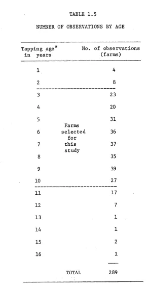
1.4.4 Samples for the present study

Of the 289 rubber smallholdings surveyed, 249 were selected for analysis in the present study. These selected farms were planted with either budgrafts of clone PB86 or selected seedlings of Tjir 1. The

trees were within the age groups of three to ten years of their period of tapping. This period corresponds to the first of the three equal periods of ten years of the entire exploitation cycle observed by Lim

(1972).

The number of farms in each age group are presented in Table 1.5. The data gave no variation of age of trees within each farm. The number of farms selected in each age group varied from a minimum of 20

in year 4 of tapping to a maximum of 39 in year 9. The number of observations selected for each age group is quite evenly spread.

Farms in the age groups 1 and 2 were rejected because of small samples and inconsistency in the recorded output. Likewise, farms in the age groups 11 and above were rejected because of small sample size. In addition, tapping in these farms would have been carried out on renewed bark, and Lim (1972) has shown that yield patterns on the

NUMBER OF OBSERVATIONS BY AGE

Tapping age in years

No. of observations (farms)

1 4

2 8

3 23

4 20

5

Farms

31

6 selected 36

for

7 this 37

8

study

35

9 39

10 27

11 17

12 7

13 1

14 1

15 2

16 1

TOTAL 289

CHAPTER 2

AVERAGE AND FRONTIER PRODUCTION FUNCTIONS: THEORETICAL CONSIDERATIONS

2.1 The Production Functions

A production function is a mathematical expression showing the

transformation of a given set of inputs into a set of outputs. Numerous

algebraic forms may be used and there is no presumption that a single form should be used to characterise agricultural production under all

environmental conditions. Various functional forms have been discussed

in detail by Heady and Dillon (1961).

Yotopoulos (1967) has pointed out the difficulties underlying the choice among alternative functional forms:

It is difficult to establish empirically that a functional form adequately describes the logic and

the mechanics of the production process. Yet, research

of nearly four decades in this field has established a strong presumption that a number of functions are competent initial approximations of the 'true’ form. Among those functions a comfortable choice of a specific algebraic form can be made on the basis of its

theoretical implications and its computational manage­ ability .

In this study, the unrestricted Cobb-Douglas form, that is, an

equation linear in the logarithms of the variables, was chosen partly for its ease of manipulation and interpretation and for its good fit to the data; and more importantly, its log linear form permits easy calculation of the "frontier" production function by the application of a conventional

linear programming package. Several other forms were tried such as

Some other forms, such as CES functional form could have been chosen for the purpose, but with more than two factors of production, the CES function becomes quite complicated and it is not possible to estimate using a linear programming technique.

Having selected the appropriate functional form, two different methods

of fitting the function are applied: the ordinary least squares method

which estimates an average function; and the linear programming method which estimates the frontier or best production function.

Muller (1974) has suggested that the concept of the "frontier" is relative and artificial:

. . . To add more of one input, i.e., production knowledge, should of course, increase output, so the frontier function can at best be defined with respect to a fixed level of information only, or for that matter, at any fixed level of other

left-out factors. Once all inputs are taken into account,

measured productivity differences should disappear

except for random disturbances. In this case the

frontier and the average function are identical. They only diverge if significant inputs have been left out in the estimation.

Due to data limitation, it is not possible to include all the inputs

as suggested by Muller. Those factors which are commonly associated with

management and "information" as defined by Muller were not available.

2.2 Properties of the Cobb-Douglas Function

The Cobb-Douglas functional form commonly used is:

b . b

where

q3 = b

X . . ... x ... x .

o lj ij nj

h

is the output of farm j

X. . is the factor input i used by farm

b is the constant

o b.

i is the parameter associated with the

For c o m p u t a t i o n a l purposes, this f orm b e c o m e s linear in logari t h m s

of the variables. Thus (2.1) can be w r i t t e n in log (capital letters)

linear f orm as

-Q. = b + b.x,. + ... + b.x.. + ... + b x . ...(2.2)

o i ij l ij n nj

The m a r g i n a l p r o d u c t of each input factor is the p a r t i a l d e r i v a t i v e

of the output w i t h r e s p e c t to an input, w i t h all o ther inputs h eld constant.

Thus, d i f f e r e n t i a t i n g the f u n c t i o n (2.1) w i t h r e s p e c t to one input, x^,

w e h a v e :

M P x . = _9<^ ,

1 9x.

l

b .b x 1

l o 1

b -1 x . i

l xbnn

i x (2.3)

Since is the m e a s u r e of a v e r a g e product, e q u a t i o n (2.3) shows X ,

1 th

that the m a r g i n a l p r o d u c t of the i input is equal to the a v e r a g e pro d u c t

m u l t i p l i e d by its exponent.

T he e l a s t i c i t y of p r o d u c t i o n of e ach input is d e f i n e d as the p e r c e n ­

tage c hange in ou t p u t for a one per cent ch a n g e in that input, w h i l e the

o ther input levels are h eld constant. The m a r g i n a l p r o d u c t is e m p l o y e d

in d e r i v i n g the e l a s t i c i t y of produc t i o n .

The o utput e l a s t i c i t y of the itn input factor, qxi, is:

i = ^

qxi 9x-

fi

q

q i

[b, — —

i x ± q

(2.4)

Therefore, the c o e f f i c i e n t s b^ (i = 1 , 2 , ...n) are the e l a s t i c i t i e s

of produc t i o n , and e ach of these r e m a i n s c o n s t a n t t h r o u g h o u t the p r o d u c t i o n

The degree of homogeneity of the function and the returns to scale are measured by the sum of the elasticities of production. Hence, if

n

^L^b^ is greater than unity, there are increasing returns to scale; if it is less than one, decreasing returns to scale occur. If the sum of the exponents is equal to one, there are constant returns to scale.

Marginal productivity changes for different levels of input can be derived from equation (2.3). The second derivative of (2.3) gives:

l!a. = b . (b i) q ... (2.5)

3x2 1 1 x?

i i

which is negative since b^<l. Thus we have diminishing marginal productivity for increasing input levels.

Under the assumption of perfect markets, the equilibrium condition is the point at which the marginal value product of each of the resources is equal to its marginal cost. The first order condition for profit maximization is that the marginal product of each factor is equal to the ratio of the price of the factor and the product. Hence, for the ith factor, profit maximization occurs when

MP =

xi 3x. *

l x .

l

(

2

6

where

P . is the price of the it^1 factor xi

PQ is the price of the product

Under the assumption of perfect markets, direct comparison between the marginal productivity of a factor and its opportunity cost will measure the existence of resource misallocation of a particular firm in

In spite of the many attractive properties of the Cobb-Douglas

function, there are a few drawbacks. One of the most limiting character­

istics is that the function assumes a constant and unit elasticity of

substitution between the input factors. Nevertheless, as long as we

keep the limitations of this functional form clearly in mind, we can always exercise the necessary caution in interpreting its results.

2.3 Ordinary Least Squares Procedure

In order to estimate the Cobb-Douglas function, the log linear form

of equation (2.2) is used. Since this estimation is made from a sample,

an error term is introduced. The equation (2.2) becomes:

Q = b + b^x. + ... + b.x. 4- ... b x + U .... (2.7)

o i l l i n n

where U is the stochastic error term.

Equation (2.7) now expresses the exact linear relationship between the dependent variable Q and the n explanatory or independent variables

x^, x^ .... and the error term U which may be composed of measurement

error and/or error due to the omission of certain variables.

Ordinary least squares method is used to estimate the unknown

parameters b^ (i = 0, 1, 2, .... n) and the error distribution. The

sample estimates of equation (2.7) are

Q = b + b 1x 1 + ... b..x + ... b x + U .... (2.8)

x o 1 1 1 1 n n

The least squares method of estimation is unbiased given the following assumptions:

(a) the error terms are random with zero mean;

(b) the error terms are uncorrelated and have a common variance 0 2 ;

(c) the explanatory variables are not correlated with the error

terms ;

(d) the number of observations is greater than the number of

This method has been well discussed in many econometric text

books e.g. Johnston (1963); Dhrymes (1970); Koutsoyiannis (1973).

2.4 Frontier Production Function

The Cobb-Douglas function, estimated by ordinary least squares which minimises the sum of squares of the error terms on both sides of the estimated function could only represent the average function. The linear programming technique minimises the sum of squares of the

error terms all constrained to one side of the function; hence, the

frontier or the best function. It expresses the maximum product

obtained from the combination of factors at the existing state of technical knowledge.

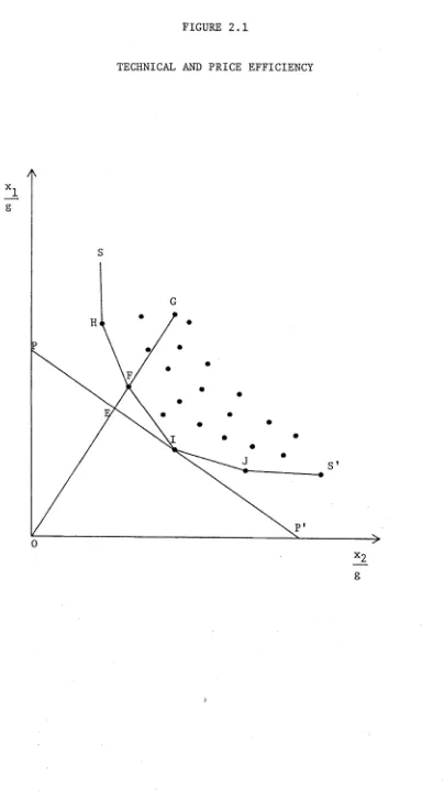
Farrell (1957) pioneered the method of estimating an efficient production function which is illustrated in Figure 2.1, for the two

inputs, one output case (Seitz,1970). Under the assumption of constant

returns to scale, the production function can be specified in the form

of a unit isoquant. Each observation represents the input combination

used by a single firm to produce one unit of output. The curve SS' is

the locus of points indicating the minimum quantities of the factors of production required to produce one unit of output with varying factor

proportions. This curve thus represents the frontier and no observation

lies between this curve and the origin, 0. All those firms which lie

on the frontier, such as H,F,I,J are said to be 100 per cent technically

efficient; those lying above S S ' are technically inefficient. Physical

or technical inefficiency of observation G is defined as the ratio of the distance between the origin and point F to the distance between the

OF

origin and the point G, i.e. — . On this basis, all firms will have a

U b

technical efficiency rating of 1 or less. The points G and F are on

FIGURE 2.1

TECHNICAL AND PRICE EFFICIENCY

If P P ’ represents the isocost line, the price inefficiency of F is the ratio of the distance between the origin and point E to the

OE

distance between the origin and point F i.e. — . In this respect, although firm F is technically efficient, it is not price efficient; hence, firm F is not economically efficient.

The firm represented by the point I, is both technically and price efficient as the isocost line PP ’ is tangent to the efficient unit isoquant S S ' at I. Hence firm I is economically efficient.

Technical efficiency is measured in relation to those firms at the frontier whereas price efficiency is measured in relation to the isocost line. The product of these two separate efficiencies,

OF OE = OE OG X OF OG *

measures the economic efficiency of the firm at G.

Given the Farrell techniques, and since technical efficiency is measured in relation to those firms on the frontier, any additional observations may reduce but cannot increase the technical efficiency of a given firm. However, additional observations may change the slope of isoquant SS' and the slope of isocost line P P 1 on which the price efficiency depends; hence price efficiency is more sensitive to additional observations and also to errors in factor prices. It was decided not to measure price efficiency because accurate price data were not available.

Nerlove (1965) and Bressler (1967) criticised Farrell’s method because it utilises only the ''marginal" observations and operates in an input-input space under the assumption of constant returns to scale which raised a number of theoretical and operational difficulties.

constraining errors to one sign and fitting least lines with linear programming technique, a fitted envelope function could be obtained using all observations in the estimation. This method operates in the output-input space and the assumption of constant returns to scale need not be made.

The analysis in this study uses the Aigner and Chu method which has been clearly explained by Timmer (1970).

2.4.1 Method of Estimation of Frontier Production Function The Cobb-Douglas model in general form, linear in logarithm, given by equation (2.7), can be written as:

Qj ' i S o V i j + (2.9)

where one column of x_^ is a vector of ones to allow for an intercept.

To make this a frontier function all U. must be constrained to

J

one side of the estimated production surface. Thus, the production function (2.7) should be estimated such that:

.£ b .x .. = Q. > Q. .... (2.10)

i = o i i j J J

Only "efficient" firms satisfy the final equality - all others have a small actual output than would be achieved if they too were efficient by the standard of the estimated production function. The criterion used here is to minimise the linear sum of the errors, i.e. minimise:

m m n

£ u = £ £ b x — £ q

j=l j j=li=o i ij j = r j

(

.

)

subject to

i^oViJ

5

Qj

b . > o

l

£

For any particular data set - is a constant, and hence can be dropped from the equation (2.11). Minimising (2.11) is the same as minimising:

m n

.£ £ b.x. . .... (2.13)

j =li=o 1 1J

Dividing (2.13) by m farms, the number of observations, the objective function becomes:

n i b.x.

1=0 1 1

/ \ — /V — b + b,x, + b 0x 0 +

o 1 1 2 2 + b x n n where

-X- = x. . and x = 1 i mj=i ij o

The problem then is to minimise the object function:

b + b x + b x + o 1 1 2 2

subject to the linear constraints

+ b x n n

A A A

b + b,x, , + b„x„. + ___. . . . + b x > Q,

O 1 11 2 21 n nl U

/s A A A

b + b-,x, » + b 0x A„ + ___. . .. + b x „ > Qo

0 1 12 2 22 n n2 y 2

If If If II ft

If II II It ft

If If II If ft

/s A A

b + b, x n + b~x~ + ______ + b x > Q

o 1 lm 2 2m n nm m

(2.14)

(2.15)

(2.16)

and

b i > 0

This can be solved by a linear programming package.

2.5 Estimation of Technical Efficiency

and the best functions so estimated will enable us to predict the average and the maximum physical output levels that could be obtained from each possible input combination. The efficiency level of each farm relative to the average farm is measured by the ratio of the actual observed output to the output predicted from the average production function. Similarly, the efficiency level of each farm relative to the best farm is measured by the ratio of the actual observed output to the output predicted from

the best production function.

Efficiency index

_qi

b

Antilog of (Q. -

V

where

(2.17)

Q

/N

Q

j j

is the log of the observed output of the j farm

is the estimated output level from the average or the best function.

Is there any relationship between these two methods of computing technical efficiency? Will the farm that is most technically

CHAPTER 3

RUBBER CULTIVATION AND FACTORS AFFECTING RUBBER PRODUCTION

3.1 Cultivation of Rubber

The Para rubber, whose Botanical name is Hevea brasiliensis belongs to the Euphorbiaceae family. The rubber tree grows to about 60 feet high. The bark is of variable colour, which is mainly light brown. The tree sheds its leaves once a year, in a process commonly known as "wintering" which may last for about two months.

The rubber tree will grow well in the area ten degrees north or south of the equator. It needs a rainfall in the region of 100 inches a year, and an average temperature of 75 to 85 degrees fahrenheit. The tree will not flourish in waterlogged soil, or at heights above 2,000 feet. In general, the most suitable soils for rubber are loamy, naturally drained, sandy clays, rich in mineral nutrients and organic matter. However the rubber tree is a very hardy plant and able to adapt to a very wide range of soil conditions and topography of the land.

After clearing the ground, the young plants can be planted out.

The conventional practice is to germinate the seeds in a germination bed, and the young seedlings planted in the nursery. After the young plants have been about a year in the nursery, they are transferred to their permanent positions in the field. After preparing and pegging out the land, planting out is always done in the rainy season. This is to avoid desiccation of the young plants before the roots can take hold and also to minimise the "transplanting shock". However, modern techniques have bypassed the nursery stage and the seedlings are planted straight in the field; budgrafting is carried out in the field when the young plants are about a year old.

In the field, the number of trees planted is generally in excess of the number which will eventually be allowed to mature for tapping. Tfye number of trees will be thinned down both by natural losses such as wind damage or pest attack, and also by selective thinning. Only the most

vigorous plants are allowed to remain. Budgrafted trees, and trees planted from selected seedlings are planted at different distances apart. This distance normally varies from 20 feet by 20 feet to 14 feet by 14 feet. The table below shows the planting distances and the approximate number of trees in an acre or the planting density.

Planting Distance (feet)

Number of Trees per acre

30 x 30 48

20 x 20 108

20 triangle 125

14 x 14 222

12 x 12 302

In a well-managed estate, by the time the trees are ready for tapping, only some 100 to 120 trees remain in an acre after progressive elimination of all but the best specimens. On smallholdings, using low-priced or family labour, however, densities of up to 200 trees per acre may be appropriate.

During the period of establishment, suitable ground cover of

vegetation, mainly creeping legume plants known as cover crops are planted between the rows of young rubber trees in most estates. The cover crops are to serve two main functions, namely, to combat erosion, especially immediately after clearing the jungle, and it is believed that legume plants are beneficial to the growth and establishment of the young rubber trees. In the case of smallholdings, the space between the rows of young rubber trees when they are still not productive may be used for growing cash crops such as peanuts, maize, vegetables, or sometimes tapioca and sweet-potatoes. When the rubber trees are planted on sloping ground, terraces are made following the contours. The trees are planted on the terraces. Suitable fertilizers are necessary to keep the trees in a good condition, especially during the establishment period of the first six years.

difficulties encountered in establishing rubber plantations in South America, even though it is the original home of hevea. Fortunately for

countries in South East Asia, the disease is not found in the region, and stringent precautionary measures are taken to prevent the spread of this disease to this part of the world.

3.1.1 Planting Materials

Planting materials are usually obtained from a clone or from selected seedlings.

All trees obtained by vegetative propagation from a single mother tree, either directly or by multiplication, are said to constitute a clone. The clone is then given a name, which is merely that of the mother tree, e.g. Prang Besar 86, Avros 49, Tjirandji 1, etcetera. Budding with high- yielding clones, especially carried out on good root stock, has made it possible to double, and even treble, yields as compared to the ordinary unselected trees.

The process of budding consists of removing a bud or "eye" from a branch of high-yielding rubber tree of verified quality, and inserting it under the bark of the lower stem of a young tree. If the budding is successful, a branch is produced. The part of the tree just above the branch growing out of the bud is cut off. Only this branch develops; it grows upwards and ultimately becomes the trunk of the mature tree.

Selected seeds may have come from several sources:

(a) natural random pollination of flowers of a high-yielding tree. Seeds thus obtained are sometimes called illegitimate seeds;

(c) by artificial cross-pollination of high-yielding trees, the result of which is called legitimate seeds.

These three types of seeds produce trees superior in quality to those obtained from unselected seeds. Legitimate seeds give the best seedlings, and clonal seeds come next, followed by the illegitimate variety.

3.1.2 Exploitation of the Rubber Trees

The latex is contained in a network of capillary tubes, or latex vessels, in the bark of the trunk. The vessels exist in a series of concentric rings. They are mostly concentrated near the cambium or the generating tissues in a layer 2 mm to 3 mm thick. Exploitation, or tapping, is a process of extracting rubber by making an incision in the bark of the tree. The latex vessels are opened, and a high turgor pressure in the bark tissue and latex vessels forces out a milky liquid known as latex.

Immediately after tapping, latex flow is rapid, but it slows down progressively. The flow ceases in about two to five hours, depending partly on the surrounding air temperature. The flow finally stops, due to the formation of a barrier known as a "plug" in the cut latex vessels. The last portion of the exuded latex coagulates over the incision. The latex, deposited in a cup fastened to the trunk of the tree, is then collected. If it is left to stand, the latex coagulates, so it is normally collected and processed without delay. However, there will be still some "late dripping" from the vessels. The material coagulates through natural process and is collected in the next tapping round. This forms lower grade rubber known as "scrap".

While growth-vigour is not necessarily correlated with production

efficiency, there is a definite indication that trees with larger girth produce relatively more latex, the larger circumference being associated

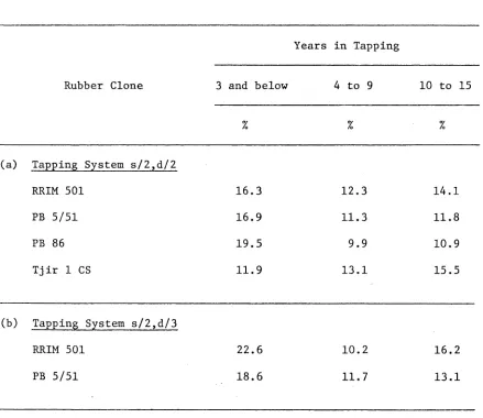
with a larger number of latex vessels in the bark. The quantity of the

lower grade rubber varies according to clones, age, and tapping system

adopted. Table 3.1 shows the weight of scrap, as a percentage of the

weight of the rubber sheets, according to planting materials and tapping systems.

TABLE 3.1

WEIGHT OF SCRAP AS A PERCENTAGE OF THE WEIGHT OF RUBBER SHEETS

Rubber Clone

Years in Tapping

3 and below 4 to 9 10 to 15

% % %

(a) Tapping System s/2,d/2

RRIM 501 16.3 12.3 14.1

PB 5/51 16.9 11.3 11.8

PB 86 19.5 9.9 10.9

Tjir 1 CS 11.9 13.1 15.5

(b) Tapping System s/2,d/3

RRIM 501 22.6 10.2 16.2

PB 5/51 18.6 11.7 13.1

Source: Extracted from Economics and Planning Division Report No. 7,

Latex is regenerated after the initial tapping. If the wound is reopened successively, the amount of latex obtained becomes more abundant. It is this special characteristic of hevea known as "wound response" which means that these trees can be exploited throughout the whole year. Since

the latex flows more freely from the tree in the morning, tapping is usually carried out in the early hours of the morning.

Tapping is an operation requiring great care and great skill; the yield of latex depends upon the length and depth of the cut. If the cut is not deep enough, the full quantity of latex is not obtained; and if it is too deep, it may damage the cambium layer on which the growth of the tree depends. The actual incision is made with a gouge or a special knife. The cut itself slopes from left (high) to right (low) at 20 to 30 degrees to the horizontal. At its lower end, the cut is extended into a vertical channel, terminating in a metal spout. Below this is attached a cup for collecting the latex. At each successive tapping, the tapper reopens the groove by removing, along its lower edge, a shaving of bark about one-sixteenth of an inch thick and the latex begins to flow again. Depending on the skill and speed of the tapper, he may visit as many as 500 to 600 trees in a morning; the number of trees he taps on a tapping day is known as his "task size".

The trees are usually in their sixth or seventh year after planting when tapped for the first time. The economic life of a tree is considered to be about thirty years of tapping. After this period, there is no more tappable bark reserve, or the yield is too low to justify further

exploitation.

Continuous research into the physiology of rubber trees has led to the discovery of methods of stimulating the yield by the application of chemical substances known as yield stimulants. Recent development of soil and leaf analysis techniques now enable more effective fertilizer use, with

applications being tailored to actual requirements instead of following a general guide. Progress in these directions, together with that due to selection, are an assurance of considerable advances in the future.*

3.1.3 Commercial Rubber Sheets

The latex collected in the cups is bulked and transported to

processing centre. The dry rubber content in the latex is normally around 30 percent.

In the processing centre, the latex is coagulated and rolled into sheets. After drip-drying, these sheets are hung in a smokehouse for the purpose of impregnating the sheets with creosote-like substances which act as preservatives. After drying, the sheets are graded in various qualities on the basis of appearance, taking into account the existence of bubbles, blemishes, black spots, mottling, etcetera. The sheet rubber is then known commercially as RSS, that is, ribbed smoked sheets. The various grades of RSS are indicated by numbers from No. 1, the standard quality, to N o . 5, the inferior fair average quality. An efficient plantation factory usually turns out more than 90 percent of No. 1 quality.

Smoked sheets are prepared by smallholders along the same lines but using crude, manual methods, a hand-operated mangle and a crudely

constructed smokehouse. Those smallholders who do not have the facility

of smokehouse may sell their rubber as unsmoked sheets. The RSS from

smallholders are usually of inferior quality.

3.2 Factors Affecting Rubber Production

The physical annual outputs from smallholder rubber production are believed to be basically influenced by the following factors:

(i) Annual inputs controlled by the smallholder in a particular

ye a r :

L Labour input in tapping rubber trees;

P Supplementary inputs such as fertilizers, weeding,

insecticides;

M Management factor;

W Type of tapping.

(ii) Lagged values of the annual inputs applied in the previous

years:

X Planting density;

B Land input of the farm;

G Age of the trees;

V Clone or variety of rubber;

D Distance of the tapper's house from the farm and

distance from the "buying" centre.

(iii) Completely exogenous variables both current and lagged:

T Topography of the farm;

S Soil type(s);

Mathematically, the above might be expressed as:

Q = f(L,P,M,W,X,B,G,V,D T,S,C) .... (3.1)

where Q is the total output of rubber from the farm in that particular year. Total output of rubber is made up of rubber sheets and scrap.

3.2.1 Annual inputs controlled by the smallholder

Annual inputs are under the immediate control of the farmer and can be changed at any time.

3.2.1.1 Labour input in tapping rubber trees

Rubber is a labour intensive crop. This is recognised in all the standard works on rubber cultivation, and on the management of rubber estates.* There seems to be no way that harvesting of the rubber, that is, tapping of rubber trees, could be conveniently mechanised.

Labour inputs can be divided into a number of operations which can be grouped into those relating to the establishment period (digging, planting, bud-grafting), maintenance period (weeding, fertilizer

application, pest and disease control), harvesting (tapping the trees) and processing the latex into sheets and delivering to the buying centre. Establishment and maintenance labour inputs of earlier periods will have a strong influence on current output. Variations in these inputs are likely to be highly correlated to managerial skill. It is the substantial time lag (six years, in the case of establishment, and one to two years in the case of maintenance inputs) between these inputs and the resultant output that prevents a single year's cross-section data on labour inputs to adequately measure the labout input in a production function.

A _{For example, see Handbook of Rubber Production published by}