arXiv:quant-ph/0004015v1 4 Apr 2000
Geometric Quantum Computation
Artur Ekert
Marie Ericsson
∗Patrick Hayden
Hitoshi Inamori
Jonathan A. Jones
Daniel K. L. Oi
Vlatko Vedral
Centre for Quantum Computation
University of Oxford
Clarendon Laboratory, Parks Road
Oxford OX1 3PU, UK
February 1, 2008
Abstract
We describe in detail a general strategy for implementing a conditional geometric phase between two spins. Combined with single-spin opera-tions, this simple operation is a universal gate for quantum computation, in that any unitary transformation can be implemented with arbitrary precision using only single-spin operations and conditional phase shifts. Thus quantum geometrical phases can form the basis of any quantum computation. Moreover, as the induced conditional phase depends only on the geometry of the paths executed by the spins it is resilient to certain types of errors and offers the potential of a naturally fault-tolerant way of performing quantum computation.
1
Introduction
Among the surprising effects recently discovered in quantum mechanics is that a quantum system retains a memory of its motion when it undergoes a cyclic evolution [1]. This is reflected in the existence of the Berry phase, a phase acquired by the quantum state of the system in addition to the better known dynamic phase. The Berry phase is a purely geometrical effect that can be linked to the notion of parallel transport [2]: it depends only on the area covered by the motion of the system, and is independent of details of how the motion is executed. Berry phases have been demonstrated in a wide variety of systems [3], including NMR [4, 5], the closely related technique of NQR [6–8], optical systems [9], and others.
∗Department of Quantum Chemistry, Uppsala University, Box 518, Se-751 20 Uppsala,
An equally exciting recent development in the field of quantum mechanics has been the discovery that quantum systems can be used to perform novel information processing tasks, including computations which are more efficient than any algorithm known on a classical computer [10–12]. Quantum informa-tion processing requires the ability to execute condiinforma-tional dynamics [13] between two quantum bits (qubits), where the state of one qubit influences the evolution of another qubit during a quantum computation. Simple quantum information processing has been demonstrated using NMR [14–17] and trapped ions [18].
Recent experimental work has managed to combine these two quantum phe-nomena in the form of geometric quantum computation [19]. (For a more ab-stract approach see [20,21].) In this paper we seek to detail the theoretical ideas behind geometric quantum computation. In particular we show that Berry’s phase may be used to implement conditional phase shifts, and thus any quan-tum gate [24]. We begin with brief introductions to both quanquan-tum gates and networks as well as to geometric phases, proceeding to analyse the dynamics of a spin-half system in order to see in detail how the theory of geometric phases applies there. Finally, we extend the ideas to pairs of spin-half particles, showing how to introduce a conditional geometric phase between the two particles.
2
Phase gates and quantum computation
2.1
Qubits and networks
Aqubitis a quantum system in which the Boolean states 0 and 1 are represented by a prescribed pair of normalised and mutually orthogonal quantum states labeled as {|0i,|1i}. Unlike a simple Boolean variable, a qubit, typically a microscopic system such as an atom, a nuclear spin, or a polarised photon, can exist in an arbitrary superpositionα|0i+β|1i, making it more powerful as a computational resource.
In quantum computation, we set someregister of qubits to an “input” state, evolve the qubits unitarily using simple building-block operations and then take the final state as “output”. More formally, a quantum logic gate is a device which performs a fixed unitary operation on selected qubits in a fixed period of time and aquantum networkis a device consisting of quantum logic gates whose computational steps are synchronised in time [23]. The outputs of some of the gates are connected by wires to the inputs of others. Thesizeof the network is the number of gates it contains.
2.2
Quantum logic gates
The most common quantum gate is the Hadamard gate, a single qubit gateH
performing the unitary transformation known as the Hadamard transform. It is defined as
H= √1
2
1 1 1 −1
|xi H (−1)
x|xi+|1−xi
√
The matrix is written in the computational basis{|0i,|1i}and the diagram on the right provides a schematic representation of the gateH acting on a qubit in state|xi, withx= 0,1.
The addition of another single qubit gate, the phase shift gateφ, defined as
|0i 7→ |0iand|1i 7→eiφ|1i, or, in matrix notation,
φ=
1 0 0 eiφ
|xi
φ
eixφ|xi (2)
is actually sufficient to construct the following network (of size four), which generates the most general pure state of a single qubit (up to a global phase),
|0i H 2θ H
π
2 +φ
cosθ|0i+eiφsinθ|1i. (3)
Consequently, the Hadamard and phase gates are sufficient to construct any
unitary operation on a single qubit.
Thus the Hadamard gates and the phase gates can be used to transform the input state|0i|0i...|0i ofn qubits into any state of the type|Ψ1i |Ψ2i... |Ψni,
where|Ψiiis an arbitrary superposition of|0iand|1i.These are rather special
n-qubit states, called the product states or the separable states. In general, a register ofn qubits can be prepared in states which are not separable, known as entangled states.
However, in order to entangle two or more qubits it is necessary to have access to two-qubit gates. One such gate is the controlled phase shift gateB(φ) defined as
B(φ) =
1 0 0 0 0 1 0 0 0 0 1 0 0 0 0 eiφ
|yi
|xi
φ
eixyφ|xi |yi. (4)
The matrix is written in the computational basis{|00i,|01i,|10i, |11i} and the diagram on the right shows the structure of the gate.
2.3
Universality
An important result in the theory of quantum computation states that the Hadamard gate, and all B(φ) controlled phase gates form a universal set of gates: if the Hadamard gate as well as all B(φ) gates are available then any
n-qubit unitary operation can be simulated exactly with less thanC4nnsuch
3
Geometric phase
3.1
Cyclic evolution
The states of a quantum system are usually described as being represented by vectors of norm 1 (|hψ|ψi|2= 1) in a complex Hilbert spaceH. However, there
is redundancy in this description since the state|ψiis physically indistinguish-able from the state eiφ|ψi. It is therefore convenient to consider instead the
projective spaceP, in which vectors are grouped into equivalence classes under the relation|ψi ∼ reiφ|ψi for any r > 0 and real φ, thereby eliminating the
ambiguity. The associated projection map is Π : H → P
|ψi 7→ [|ψi] =
|ψ′i:|ψ′i=reiφ|ψi . (5)
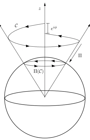
If a system undergoes a cyclic evolution, the ket representing the system state traces out a path,C: [0, τ]−→ H, where Π(C) is a closed curve in P, as illustrated in Figure 1. In other words, the initial and final states should be on the same ray in H, but may be related by a phase, eiφ. We will measure this
phase with respect to a reference curve inH: for each point|ψ(t)ionC, we can choose a smoothly varying representative
ψ˜(t) E
from Π(ψ(t)) in such a way that
ψ˜(0) E
= ψ˜(τ)
E
. We can then write
|ψ(t)i=eif(t) ψ˜(t)
E
(6) so that the phase change of|ψ(0)iassociated with the cyclic evolution is given byφ=f(τ)−f(0).
3.2
Dynamic and geometric phase
The time evolution of a quantum system is governed by the Sch¨odinger equation,
i~d
dt|ψ(t)i=H(t)|ψ(t)i, (7)
whereH(t) is the Hamiltonian. Substituting Eq. (6) into the above, rearranging and multiplying byhψ(t)|gives the following [25],
df(t) dt =−
1
~hψ(t)|H|ψ(t)i+i
D
˜
ψ(t)
d dt
ψ˜(t)
E
, (8)
or, when integrated,
φ=−~1 Z τ
0 h
ψ(t)|H|ψ(t)idt+i
Z τ
0
D
˜
ψ(t)
d dt
ψ˜(t)
E
dt. (9) Thus,φcan be decomposed into a dynamical phase
δ=−1~ Z τ
0 h
eiφ
z
Π
C
[image:5.612.214.399.220.507.2]Π(C)
which depends on the Hamiltonian, and a geometric phase
γ=i
I C D ˜ ψ d ψ˜ E (11) which depends only on the pathC;γis independent of the rate at which|ψ(t)i
progresses alongC, the Hamiltonian, or the choice of referencen ψ˜
Eo
.
3.3
Berry’s phase
A particular instance of this geometric phase is Berry’s phase [1], which occurs when the adiabatic theorem (see [26]) is satisfied. In this case, if the initial state
|ψ(0)iof the system is an eigenstate of the Hamiltonian, the state|ψ(t)iremains an eigenstate|ψ(t)i=|n(R)iof the instantaneous HamiltonianH(R), where Ris a set of time-varying parameters controlling the Hamiltonian. SupposingR
traces a closed loop in the parameter space, the geometric phase of the system can be written in terms ofR. In this case, provided the energy eigenspace of the
instantaneous Hamiltonians is non-degenerate along the pathC, the geometric phase acquired by thenth-eigenstate is
γn=i
I
C
D]
n(R) ∇R ]
n(R)E·dR, (12)
where ∇R is the gradient operator with respect to the parameters R, and
]
n(R)E is defined as in the previous section. This line integral can be
trans-formed into a surface integral over any surface in the parameter space whose boundary isC.
Since experimentally it is much easier to control the Hamiltonian than the actual state of a system, the adiabatic case is of importance. However, the adiabatic conditions necessarily mean that the processes take a long time com-pared to the characteristic dynamical time-scales, and thus are much slower than dynamic methods of generating phases.
4
Single-qubit evolution
4.1
Qubit Dynamics
Here we will focus on developing an understanding of the time evolution of a single qubit governed by a very general Hamiltonian. Recall that any 2×2 Hermitian matrix can be written in terms of the unit matrix and the three Pauli matrices. In particular a single qubit density operator can be parametrised as
ρ= 1
2(1+s·σ) = 1 2
1 +sz sx−isy
sx+isy 1−sz
, (13)
where the real vectors= (sx, sy, sz) is known as the Bloch vector. By the same
token any 2×2 Hamiltonian can be written as
H = ~
Ω
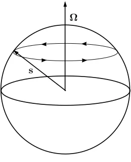
[image:7.612.238.370.123.286.2]s
Figure 2: Solution to the equations of motion for a single spin-half particle.
whereΩ is called the Rabi vector. Substituting Eq. (13) and Eq. (14) into the
equation of motion for the density operator,
i~d
dtρ= [H, ρ] (15)
and using the identity
(a·σ)(b·σ) = (a·b)1+i(a×b)·σ, (16)
we find the following equation of motion for the Bloch vector, d
dt s=Ω×s. (17)
This equation has a simple geometric solution: vectorsrevolves around vector Ωwith angular frequency given by|Ω|, the length ofΩ, as illustrated in Figure
2.
From Eq. (17), it is relatively easy to move to situations typical of those encountered in quantum computation. Hamiltonians that describe qubits in-teracting with external potentials are usually time dependent. Typical exter-nal perturbations are periodic such as, for example, spins coupled to oscillating magnetic fields in NMR or atomic dipole moments coupled to oscillating electro-magnetic field in the optical domain. Within the Rotating Wave Approximation the oscillating field can be replaced by a rotating field, and so the Hamiltonian is of the form
H(t) =~ 2
ω0 ω1e−i(ωt+φ)
ω1ei(ωt+φ) −ω0
, (18)
whereω0/2πis the system’s transition frequency, whileω/2πand~ω1 are the
In order to solve Eq. (17) it is convenient to consider the evolution ofs in
a frame which rotates with frequency ω around thez-axis. More precisely, we write
s(t) =Rz(ωt)s′(t), Ω(t) =Rz(ωt)Ω′(t), (20)
whereRz(ωt) is the rotation matrix
Rz(ωt) =
cos(ωt) −sin(ωt) 0 sin(ωt) cos(ωt) 0
0 0 1
= exp(ωtMz), (21)
for
Mz=
0 −1 0 1 0 0 0 0 0
. (22)
Substituting Eq. (20) into Eq. (17) and taking into account that d
dt Rz(ωt) =Rz(ωt)(ωMz), Mzs
′ = ˆz×s′, (23)
where ˆzis a unit vector in thez-direction, we obtain
d dt s
′=Ω′×s′ (24)
with the time-independent vectorΩ′,
Ω′
x=ω1cos(φ), Ω′y =ω1sin(φ), Ω′z=ω0−ω. (25)
If we can control the strength of coupling~ω1, the frequencyωand the phase
φ of the external field we can prepare any vectorΩ. This implies that if we
know the initial state of the qubit then with a single rotation we can position the Bloch vectorsin any prescribed direction.
4.2
Calculating geometric phases
We can now apply the results of the previous section to the task of developing a geometric phase of a spin-half particle located in an external oscillating field. By varying the parameters of the Hamiltonian adiabatically we will send a qubit through a cyclic evolution, whose associated geometric phase can be calculated using Eq. (11).
Working in the rotating frame, the components (Ω′
x,Ω′y,Ω′z) of the
Hamil-tonian are given by Eq. (25), where the frequency and power of the rotating field can be used to control the value of the angleθof Figure 3. In the absence of a rotating field the Rabi vector lies along the z-axis, and as the power of the rotating field is slowly increased from zero toω1the vector tilts towards the
xy-plane. If the Bloch vectors′is initially aligned withΩ′then by the adiabatic
z
s
θ
Figure 3: Spin-half particle in a magnetic field
from the relation between the different componentsΩ′ we find that the angleθ
between the Bloch vector and thez-axis will be cosθ= Ω
′
z
q
Ω′2
x + Ω
′2
y + Ω
′2
z
=p ω0−ω
(ω0−ω)2+ω12
. (26)
Varying the phase φ of the rotating field from Eq. (25) will then cause
s′ to rotate around the z-axis. The geometric phase associated with a full
revolution is easily calculated by parameterizing the state in terms of the| ↑i
and | ↓ieigenstates of quantization along the z-axis, ψ˜(α)
E
= cos(θ/2)| ↑i+ sin(θ/2)eiα| ↓i, whereαchanges smoothly from 0 to 2π. Using Eq. (11),
γ = i
I
C
cosθ
2| ↑i+ sin
θ
2e
iα| ↓i
†
d
cosθ
2| ↑i+ sin
θ
2e
iα| ↓i
= − Z 2π
0
cosθ
2h↑ |+ sin
θ
2e
−iα
h↓ | sinθ 2e
iα
| ↓i
dα
= −12(1−cosθ)
Z 2π
0
dα
= −π(1−cosθ). (27)
4.3
Eliminating dynamic phases
In order to perform conditional quantum gate operations using geometric phases only, it is necessary to find a way to eliminate the dynamic phase. One approach is to use a refocussing technique known as spin-echo. The basic idea is to apply the cyclic evolution twice, with the second application surrounded by a pair of fastπtransformations (this being simply the transformation that swaps the basis states| ↑iand| ↓i.) The net effect of this compound transformation would be to cancelall the acquired phases except that the second cyclic evolution is performed by retracing the first but in the opposite direction so that while the dynamic phases cancel, the geometric phases do not.
To see why this is so, letC↑be the closed curve inP traced out by
˜↑
E
during the first cyclic evolution andC↓ the one traced out by
˜↓
E
, with corresponding dynamic and geometric phasesδ↑, γ↑, δ↓, and γ↓. Referring back to Eq. (27)
we see thatγ↑=−γ andγ↓=γforγ =π(1−cosθ). Similarly, if we write ¯C↑
and ¯C↓for the second cyclic evolution, these are simplyC↑andC↓carried out in
opposite orientations so they have corresponding phases ¯γ↑=γ and ¯γ↓=−γ.
In summary, we can follow the states through the compound evolution as follows:
| ↑i−→C↑ ei(δ↑−γ)| ↑i−→π ei(δ↑−γ)| ↓i
¯
C↓
−→ei(δ↑+δ↓−2γ)| ↓i−→π ei(δ↑+δ↓−2γ)| ↑i | ↓i−→C↓ ei(δ↓+γ)| ↓i−→π ei(δ↓+γ)| ↑i
¯
C↑
−→ei(δ↑+δ↓+2γ)| ↑i−→π ei(δ↑+δ↓+2γ)| ↓i.
(28) Since the global phase factorei(δ↑+δ↓)is not physical this sequence of operations
behaves as promised. The dynamic phases are eliminated and we are left with an exclusively geometric phase difference of 4γ= 4πcosθ.
5
Conditional dynamics
5.1
2-Spin Hamiltonian
This geometric phase can be used to implement a 2-qubit controlled-phase gate. Consider to begin with a system of two non-interacting spin-half particles Sa
andSb. In a reference frame aligned with the static field, the Hamiltonian reads
H0=~ωaSaz⊗1b+~ωb1a⊗Sbz, (29)
or, in the basis{|Saz, Sbzi}Saz,Sbz ={| ↑↑i,| ↑↓i,| ↓↑i,| ↓↓i},
H0=
~
2
ωa+ωb 0 0 0
0 ωa−ωb 0 0
0 0 −ωa+ωb 0
0 0 0 −ωa−ωb
, (30)
where the frequenciesωa/2πandωb/2πare the transition frequencies of the two
spins and we have used the scaled Pauli operatorsSi=σi/2. (From now on we
| ↓↓i −ωa−ωb
2
−ωa−ωb+πJ
2
| ↓↑i −ωa+ωb
2 −ωa+ωb−πJ
2
| ↑↓i ωa−ωb
2 ωa−ωb−πJ
2
| ↑↑i ωa+ωb
2
ωa+ωb+πJ
2
6 ω+
6 ω−
Figure 4: The energy diagram of two interacting spin-half nuclei. The transition frequency of the first spin depends on the state of the second spin.
If the two particles are sufficiently close to each other, they will interact, creating additional splittings between the energy levels. In the case of two spin-half particles, the magnetic field of one spin may directly or indirectly affect the energy levels of the other spin; the energy of the system is increased byπ~J/2 if
the spins are parallel and decreased byπ~J/2 if the spins are antiparallel. The
Hamiltonian of the system taking into account this interaction reads
H=H0+ 2π~JSaz⊗Sbz, (31)
or, in the previously chosen basis,
H = ~ 2
ωa+ωb+πJ 0 0 0
0 ωa−ωb−πJ 0 0
0 0 −ωa+ωb−πJ 0
0 0 0 −ωa−ωb+πJ
.
(32) Figure 4 illustrates the energy levels of the system. When spinSbis in state
| ↑i, the transition frequency of the spin Sa is
ω+=ωa+πJ, (33)
whereas when spinSb is in state| ↓i, the transition frequency of the spinSa is
ω−=ωa−πJ. (34)
5.2
Conditional phase shift
acquired by a spin depends on its transition resonance frequency as given by Eq. (26). Therefore, at the end of a cyclic evolution, the Berry phase acquired by the spin Sa will be different for the two possible states of spinSb. Indeed,
when spinSb is in state | ↑i, the Berry phase acquired by the spinSa is γ+ =
∓π(1−cosθ+), with the sign negative or positive depending on whether spin
Sa is up or down, respectively, and
cosθ+=
ω+−ω
p
(ω+−ω)2+ω21
. (35)
Similarly, when spinSb is in state| ↓i, the Berry phase acquired by the spinSa
isγ− =∓π(1−cosθ−) where
cosθ−=
ω−−ω
p
(ω−−ω)2+ω12
. (36)
As in the single-particle case, it is necessary to eliminate the dynamic phase in order to construct a purely geometric conditional phase gate. This can be accomplished using almost the same technique as in the single-particle case described in Section 4.3. In this case, however, we must apply the sequence of operations
C −→πa−→C −→¯ πb−→ C −→πa −→C −→¯ πb, (37)
whereπaandπbareπ-pulses applied to particlesaandb, respectively, andCand
¯
C are adiabatic transformations as in Section 4.3. If we define the differential Berry phase shift
∆γ=γ+−γ−=π
ω+−ω
p
(ω+−ω)2+ω12
−p ω−−ω
(ω−−ω)2+ω21
!
(38)
then the net transformation, up to global phases, is given by
e2i∆γ 0 0 0
0 e−2i∆γ 0 0
0 0 e−2i∆γ 0
0 0 0 e2i∆γ
. (39)
Thus, we have succeeded in engineering a conditional evolution since the state of the qubit Sb influences the phase acquired by a second qubitSa. [27] This
gate, which introduces a phase ofe2i∆γ if the two spins are aligned ande−2i∆γ
if they are anti-aligned, is equivalent to the controlled phase gate introduced in Section 2 [22].
5.3
Fault Tolerance
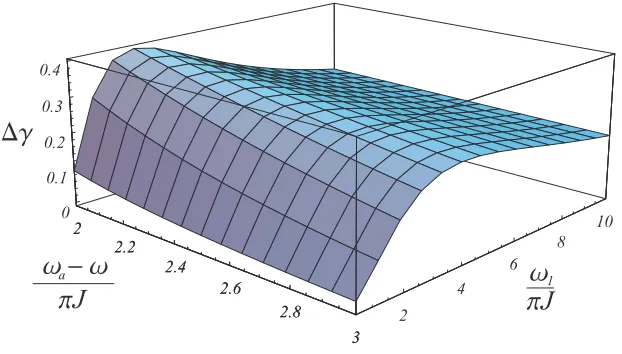
The form of the dependence of ∆γ on the detuning ωa−ω and the amplitude
Figure 5: Plot of differential phase shift ∆γ as a function of ωa−ω
πJ and
ω1
πJ.
fault tolerance not present in the simple non-geometric conditional phase gate. In many experiments, such as NMR, it is easy to control the detuning quite precisely, but relatively difficult to control the amplitude of the oscillating field. Figure 5 plots ∆γ as a function of these parameters in units ofπJ for a range of values: for fixedωa−ω, we see that there is a peak in ∆γas a function ofω1.
Therefore, ifω1is chosen to coincide with this peak then ∆γwill be insensitive
to errors inω1to first order. As the height of the peak depends on the detuning,
any desired controlled phase gate can be achieved.
6
Conclusions
7
Acknowledgments
This work was supported in part by the European TMR Research Network ERP-4061PL95-1412, The Royal Society of London, Elsag, Starlab (Riverland NV, Belgium), the European Science Foundation, CESG, and the Rhodes Trust.
References
[1] M.V. Berry, 1984,Proc. Roy. Soc. A 392, pp.47.
[2] B. Simon, 1983,Phys. Rev. Lett.51, pp.2167.
[3] A. Shapere and F. Wilczek, 1989, Geometric phases in Physics, World Scientific, Singapore.
[4] D. Suter, G. Chingas, R. Harris and A. Pines, 1987, Molec. Phys. 61,
pp.1327.
[5] M. Goldman, V. Fleury and M. Gu´eron, 1996, J. Magn. Reson. A 118,
pp.11.
[6] R. Tycko, 1987,Phys. Rev. Lett.58, pp.2281.
[7] S. Appelt, G. W¨ackerle and M. Mehring, 1994Phys. Rev. Lett.72, pp.3921.
[8] J. A. Jones and A. Pines, 1997,J. Chem. Phys.106, pp.3007.
[9] A. Tomita and R. Chiao, 1986,Phys. Rev. Lett.57, pp.937.
[10] D. Deutsch, 1985,Proc. R. Soc. Lond. A400, pp.97.
[11] P. W. Shor, 1994,Proc. 35th Ann. Symp. on Fund. of Comp. Sci.. [12] L. Grover, 1996,Proc. 28th Ann. Symp. on the Th. of Comp.pp.212. [13] A. Barenco, D. Deutsch, A. Ekert and R. Jozsa, 1995,Phys. Rev. Lett.74,
pp.4083.
[14] D. G. Cory, A. F. Fahmy, and T. F. Havel, 1996, in “PhysComp ’96” (T. Toffoli, M. Biafore, and J. Le˜ao, Eds.), New England Complex Systems Institute pp.87–91.
[15] D. G. Cory, A. F. Fahmy and T. F. Havel, 1997,Proc. Nat. Acad. Sci. USA
94, pp.1634.
[16] N. A. Gershenfeld and I. L. Chuang, 1997,Science 275, pp.350.
[17] J. A. Jones and M. Mosca, 1998,J. Chem. Phys.109, pp.1648.
[19] J. A. Jones, V. Vedral, A. Ekert, and G. Castagnoli, 2000, Nature 403
pp.869.
[20] P. Zanardi, M. Rasetti, 1999,Phys. Lett. A264pp.94.
[21] J. Pachos, P. Zanardi, and M. Rasetti,Phys. Rev. AIn press.
[22] J. A. Jones, R. H. Hansen and M. Mosca, 1998, J. Magn. Reson. 135,
pp.353.
[23] D. Deutsch, 1989,Proc. R. Soc. Lond. A425, pp.73.
[24] A. Barenco, C. H. Bennett, R. Cleve, D. P. DiVincenzo, N. Margolus, P. W. Shor, T. Sleator, J. Smolin and H.Weinfurter, 1995, Phys. Rev. A
52, pp.3457.
[25] J. Anandan, 1992,Nature 360pp.307.
[26] A. Galindo and P. Pascual, 1990,Quantum Mechanics II Springer-Verlag. [27] Animated representations of the single qubit and conditional gates can be