High resolution vertical total electron content maps based on multi scale B spline representations

https://doi.org/10.5194/angeo-37-699-2019 © Author(s) 2019. This work is distributed under the Creative Commons Attribution 4.0 License.

High-resolution vertical total electron content maps based

on multi-scale B-spline representations

Andreas Goss1, Michael Schmidt1, Eren Erdogan1, Barbara Görres2, and Florian Seitz1 1_{Deutsches Geodätisches Forschungsinstitut der Technischen Universität München,}

Arcisstraße 21, 80333 Munich, Germany

2_{Bundeswehr GeoInformation Centre (BGIC), Euskirchen, Germany} Correspondence:Andreas Goss ([email protected])

Received: 28 February 2019 – Discussion started: 4 March 2019

Revised: 11 July 2019 – Accepted: 16 July 2019 – Published: 12 August 2019

Abstract. For more than 2 decades the IGS (Interna-tional GNSS Service) ionosphere associated analysis centers (IAACs) have provided global maps of the vertical total elec-tron content (VTEC). In general, the representation of a 2-D or 3-D function can be performed by means of a series ex-pansion or by using a discretization technique. While in the latter case, pixels or voxels are usually chosen for a spheri-cal function such as VTEC, for a series expansion spherispheri-cal harmonics (SH) are primarily used as basis functions. The selection of the best suited approach for ionosphere model-ing means a trade-off between the distribution of available data and their possibility of representing ionospheric varia-tions with high resolution and high accuracy.

Most of the IAACs generate global ionosphere maps (GIMs) based on SH expansions up to the spectral degree

n=15 and provide them with a spatial resolution of 2.5◦×5◦ with respect to the latitudinal and longitudinal directions, re-spectively, and a temporal sampling interval of 2 h. In recent years, it has frequently been claimed that the spatial resolu-tion of the VTEC GIMs has to be increased to a spatial reso-lution of 1◦×1◦and to a temporal sampling interval of about 15 min. Enhancing the grid resolution means an interpola-tion of VTEC values for intermediate points but with no fur-ther information about variations in the signal.n=15 in the SH case, for instance, corresponds to a spatial sampling of 12◦×12◦. Consequently, increasing the grid resolution con-currently requires an extension of the spectral content, i.e., to choose a higher SH degree value than 15.

Unlike most of the IAACs, the VTEC modeling approach at Deutsches Geodätisches Forschungsinstitut der Technis-chen Universität MünTechnis-chen (DGFI-TUM) is based on

local-izing basis functions, namely tensor products of polynomial and trigonometric B-splines. In this way, not only can data gaps be handled appropriately and sparse normal equation systems be established for the parameter estimation proce-dure, a multi-scale representation (MSR) can also be set up to determine GIMs of different spectral content directly, by applying the so-called pyramid algorithm, and to perform highly effective data compression techniques. The estima-tion of the MSR model parameters is finally performed by a Kalman filter driven by near real-time (NRT) GNSS data.

Within this paper, we realize the MSR and create multi-scale products based on B-spline scaling, wavelet coeffi-cients and VTEC grid values. We compare these products with different final and rapid products from the IAACs, e.g., the SH model from CODE (Berne) and the voxel solution from UPC (Barcelona). In contrast to the abovementioned products, DGFI-TUM’s products are based solely on NRT GNSS observations and ultra-rapid orbits. Nevertheless, we can conclude that the DGFI-TUM’s high-resolution product (“othg”) outperforms all products used within the selected time span of investigation, namely September 2017.

1 Introduction

800 km) using increasing height above the Earth’s surface. In the case of the charge state, the atmosphere is split into the neutral atmosphere (up to a height of 80 km), the iono-sphere (about 80 to 1000 km) and the plasmaiono-sphere (above 1000 km) (see, e.g., Limberger, 2015).

The ionosphere is mostly driven by the Sun; extreme UV (EUV), X-ray and solar particle radiation cause ioniza-tion processes. In geodesy, the main ionospheric impact is the influence of free electrons on radio wave propagation. This effect mainly depends on the signal frequency, i.e., the ionosphere is a dispersive medium (Schaer, 1999). Signals with frequencies lower than 30 MHz will be blocked and re-flected by the ionosphere, whereas signals with shorter wave-lengths penetrate the ionosphere but are affected with respect to speed and direction. The ionospheric influence on radio waves is twofold: the signal travel times are changed (delay) and the signal paths are modified (bending). While the latter effect can be neglected for most applications, the ionospheric delay

dion= ± 40.3

f2 R Z

S

Neds (1)

depends directly on the electron densityNealong the signal pathsbetween satelliteSand receiverRand inversely on the carrier frequencyf. Equation (1), which can be derived from dual-frequency measurements, is only an approximation as higher-order effects are neglected. These terms depend on the magnetic field, signal frequency, signal elevation, and iono-spheric conditions and reach about 0.2 cm in zenith for GPS signals (Bassiri and Hajj, 1993). The sign on the right-hand side changes depending on whether it is applied for a carrier phase observation (“−”) or for a pseudorange measurement (“+”) (see, e.g., Langley, 1998).

Observations of space geodetic techniques, such as the global navigation satellite systems (GNSS) and the Doppler Orbitography and Radiopositioning Integrated by Satellite (DORIS) tracking system as well as satellite altimetry and ionospheric radio occultation (IRO) are based on electromag-netic signal propagation; thus, they are disturbed by the iono-sphere. Most of the techniques are not directly sensitive to the electron density, but to the integrated effect along the ray path. In Eq. (1) the integral

STEC(xS,xR, t )= R Z

S

Ne(x, t )ds (2)

is called the slant total electron content (STEC). In Eq. (2), in addition to the timetwe introduce the position vectorsxS x_Rand

x=r[cosϕcosλ,cosϕsinλ,sinϕ]T (3) of the satellite S, the receiver R and an arbitrary pointP

moving along the signal paths; the coordinate triple(ϕ, λ, r)

comprises latitudeϕ, longitudeλand radial distancerwithin a geocentric coordinate system6E.

The vertical total electron content (VTEC),

VTEC(ϕ, λ, t )=

hu Z

hl

Ne(ϕ, λ, h, t )dh, (4)

is defined as the integration of the electron density in the vertical direction, i.e., along the heighthabove the Earth’s surface, defined ash=r−RE;RE refers to the radius of a spherical Earth. Furthermore, in Eq. (4) hl andhu are the respective heights of the lower and the upper boundary of the ionosphere (see, e.g., Dettmering et al., 2011, 2014; Lim-berger, 2015).

Equations (2) and (4) require a 3-D integration of the electron density. Often a simplification is preferred which is based on the so-called single-layer model (SLM). It as-sumes that all free electrons are concentrated in an infinitesi-mally thin shell, i.e., the sphereHwith radiusRH=RE+H (Schaer, 1999), whereHis the single-layer height. As a con-sequence of this assumption and according to

STEC(xS,xR, t )=M(z)·VTEC(xIPP, t ), (5) VTEC can be transformed into STEC by introducing a map-ping functionM(z)depending on the zenith anglezof the ray path between satelliteSand receiverR. In Eq. (5) the po-sition vectorxIPP, i.e., the spherical coordinates (ϕIPP,λIPP,

RH) define the ionospheric pierce point (IPP), which refers to the geometrical piercing point of the straight line betweenS

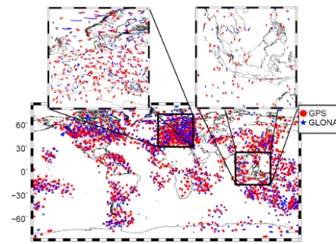
andRwith the sphereHof the SLM. This point denotes the reference point of an observation including the STEC, such as a GNSS measurement (see, e.g., Erdogan et al., 2017). Figure 1 shows, for instance, the global distribution of the IPPs from GNSS observations on 6 September 2017 between 12:55 and 13:05 UT. However, it must be pointed out that the introduction of a simple isotropic mapping functionM(z), depending solely on the zenith angle z, can only generate an approximation of STEC. Recently, more sophisticated ap-proaches, e.g., the Barcelona ionospheric mapping function (BIMF), have been developed to improve the projection of VTEC on STEC (see, e.g., Lyu et al., 2018).

Combining Eqs. (1), (2) and (5) yields the relation

dion(xS,xR, t )= − 40.3

f2 ·M(z)·VTEC(xIPP, t ) (6) between VTEC and the ionospheric delaydion in the case of a phase observation. Equation (6) can be interpreted and applied in two ways:

– if VTEC is given from an ionospheric model, the delay

dioncan be computed and used as a correction for GNSS observations;

Applications, such as satellite navigation and positioning re-quire high-precision and high-resolution VTEC models. For this purpose the correctiondioncould, according to Eq. (6), be derived from VTEC maps, usually the so-called global ionosphere maps (GIM). The most prominent GIM is pro-vided by the International GNSS Service (IGS) (Feltens and Schaer, 1998; Hernández-Pajares et al., 2011) as a weighted combination product of VTEC maps from various IGS iono-sphere associated analysis centers (IAACs), namely (1) the Jet Propulsion Laboratory (JPL), (2) the Center for Orbit Determination in Europe (CODE), (3) the European Space Operations Center of the European Space Agency (ESOC), (4) the Universitat Politècnica de Catalunya (UPC), (5) the Canadian Geodetic Survey of Natural Resources Canada (NRCan), (6) the Wuhan University (WHU) and (7) the Chi-nese Academy of Sciences (CAS). Recently, Roma-Dollase et al. (2017) published a review paper on these seven GIMs concerning their mapping techniques and their consistency during one solar cycle.

There are several modeling strategies for generating GIMs; the most prominent approach is based on spherical harmonics (SH) and was introduced by Schaer (1999). Fur-ther approaches include the tomographic approach based on voxels (Hernández-Pajares et al., 1999) and other approaches based on B-spline scaling functions and wavelets (Schmidt, 2007, 2015b; Schmidt et al., 2011), multivariate adaptive re-gression splines (MARS) and adaptive rere-gression B-splines (BMARS) (Durmaz et al., 2010; Durmaz and Karslioglu, 2015), and polynomials (Komjathy and Langley, 1996).

Generally, we distinguish between GIMs provided as “fi-nal”, “rapid”, “near real-time” (NRT) or “real-time” (RT) products. This classification is based on the latency of the underlying input data. For final products, for instance, only post-processed observations and orbits are used, whereas NRT products are based on rapid orbits and observations with a latency of some minutes up to a few hours. GIMs are typi-cally provided with a temporal resolution of 1 or 2 h and with a spatial resolution of 2.5◦×5◦with respect to geographical latitude and longitude (Hernández-Pajares et al., 2017).

VTEC variations basically follow annual, seasonal, diur-nal and semidiurdiur-nal periods. Earthquakes or incidental nat-ural hazards can also cause small but visible signatures (Liu et al., 2004; Zhu et al., 2013). However, during space weather events, such as solar flares or coronal mass ejections (CME), the number of free electrons may drastically increase. In the latter case, solar plasma consisting of electrons, ions and photons may enter the Earth’s atmosphere and cause short period variations within the electron density distribu-tion (see, e.g., Monte-Moreno and Hernández-Pajares, 2014; Wang et al., 2016; Tsurutani et al., 2006, 2009). As a con-sequence, the modeling of the disturbed ionosphere requires both a high temporal and a high spatial resolution. In 2012, during the IGS 2012 workshop in Olsztyn, Poland, it was recommended that high-resolution IGS combined GIMs be provided. The UPC and JPL IAACs agreed on

disseminat-Figure 1.Global distribution of the IPPs from GPS (red dots) and GLONASS (blue stars) measurements for 6 September 2017 col-lected within a 10 min interval between 12:55 and 13:05 UT. The regional maps at the top are “zoom-ins” of Europe and Indonesia.

ing GIMs with a temporal resolution of 15 min and a spatial resolution of 1◦×1◦with respect to latitude and longitude, respectively (Dach and Jean, 2013).

As already confirmed by Roma-Dollase et al. (2017), an increase in temporal resolution allows for an improvement in the overall accuracy of the GIMs. The authors compared the final products with a temporal resolution of 2 h with rapid products with a temporal resolution of 15 min using the dSTEC analysis, which is the most reliable method of as-sessing the accuracy of VTEC products (Hernández-Pajares et al., 2017). Following the results of their investigations, it can be stated that an increase in the temporal resolution yields better results in the dSTEC analysis.

To the knowledge of the authors, the spatial resolution of GIMs has not been investigated in detail to date. Most of the GIMs are based on series expansions in terms of SHs with a maximum degree ofnmax=15. This value fits to a block size of about 12◦×12◦on the sphereH. In contrast, a grid spacing of 2.5◦×5◦corresponds to a maximum SH degree of aroundn=36; a 1◦×1◦grid spacing, i.e., a spatial resolution of around 110 km along the Equator fits to a SH expansion up to degreen=180. As a matter of fact, a reliable com-putation of the corresponding SH series coefficients requires a global input data coverage of the same spatial sampling. As the IAAC VTEC maps are based solely on GNSS obser-vations with a rather inhomogeneous distribution (cf. Fig. 1 showing the IPPs of NRT observations with dense clusters over continents and large data gaps over oceans), finer iono-spheric structures can only be monitored and modeled where high-resolution input data are available.

signal structure (cf. Fig. 9a, c). In areas with high-resolution data, such as Europe, the US or Australia, the VTEC signal is usually rather smooth. In areas with highly variable spatial and temporal signal structures such as in the equatorial belt, a much smaller number of observations is generally given. As a consequence, for global modeling we have to deal with a trade-off between signal structure and data resolution.

It is a well-known fact that SHs as global basis func-tions are not suitable for representing unevenly, globally dis-tributed data. Consequently, in such cases, a series expansion in terms of localizing basis functions is more appropriate. In the following, we apply tensor products of polynomial and trigonometric B-splines as localizing 2-D basis func-tions. Besides the localizing features, B-splines additionally generate a multi-scale representation (MSR), also known as multi-resolution representation (MRR). The basic feature of a MSR is to split a target function into a smoothed, i.e., low-pass-filtered version, and a number of detail signals, i.e., band-pass-filtered versions via successive low-pass filtering (Mertins, 1999). Hence, a spatial MSR of VTEC adapts the model resolution to the data distribution and, thus, fulfills IGS’ requirement of high-resolution VTEC modeling.

In this study, we compare global VTEC maps based on se-ries expansions in terms of both globally defined SHs and localizing B-spline functions, including the MSR with re-spect to the re-spectral content. For this purpose, we use the SH degree as the common measure for the spectral content of a spherical signal. In detail, we study the interrelations between the SH degree, the spatial sampling intervals of the input data and the resolution levels of B-spline expansions. In addition, we discuss the influence of different temporal res-olutions of the GIMs. For the estimation of the unknown se-ries coefficients of the B-spline expansion, we use a Kalman filter (KF) procedure as explained by Erdogan et al. (2017). In order to assess the quality of the approach, we perform a dSTEC analysis (Hernández-Pajares et al., 2017).

The paper is outlined as follows: in Sect. 2 a description of VTEC modeling procedures based on both, SH and B-spline expansions are presented. In Sect. 2.3 we study the spectral resolution of global VTEC maps. Section 3 comprises a de-tailed description of the MSR and the estimation procedure. In Sect. 4 case studies are set up to verify the results of the previous sections numerically. Furthermore, this section pro-vides a final assessment by means of a dSTEC validation. The final section provides conclusions and an outlook for fu-ture work.

2 VTEC modeling approaches

The 3-D signal VTEC(ϕ, λ, t )=f (x, t ), introduced in Eqs. (4) and (5), can be modeled as series expansion

f (x, t )=

∞

X

k=0

ck(t ) φk(x) (7)

in terms of given space-dependent basis functionsφk(x)and unknown time-dependent series coefficientsck(t ).1 Assum-ing that at discrete timests=t0+s·1twiths∈N0and sam-pling interval1t the total number ofIs observationsy(xis,

ts) of VTEC at IPP positionPis ∈Hwithis=1, 2, . . . ,Is are given. Considering the measurement errorse(xis,ts), the observation equation follows from Eq. (7) and reads

y(xis, ts)+e(xis, ts)=fN(xis, ts)=

=

N X

k=0

ck(ts) φk(xis). (8)

Note, that we neglect the truncation error in the following

rN(xis, ts)=

∞

X

k=N+1

ck(ts) φk(xis) (9)

and omit other unknown parameters such as the satellite and receiver differential code biases (DCB) for GNSS geometry-free observations on the right-hand side of Eq. (8) (see, e.g., Erdogan et al., 2017).

In the following (Sect. 2.1 and 2.2), the SH expansion – as likely the most frequently used approach in ionosphere modeling – and the 2-D B-spline tensor product approach are described.

2.1 Spherical harmonic expansion

In the SH approach, the observation equation, Eq. (8), can be rewritten as

y(xis, ts)+e(xis, ts)=fnmax(xis, ts)=

=

nmax X

n=0 n X

m=−n

cn,m(ts) Yn,m(xis), (10)

where the functionsYn,m(x), i.e., the SHs of degreen=0, . . . ,nmaxand orderm= −n, . . . ,n, are defined as

Yn,m(x)=Pn,|m|(sinϕ)·

cosmλ if m≥0

sin|m|λ if m <0 (11) withPn,|m| being the normalized associated Legendre

func-tions of degreenand orderm. The total(nmax+1)2quantities

cn,m(t )in Eq. (10) are the time-dependent SH coefficients. According to the sampling theorem on the sphere, the maxi-mum degreenmaxis related to the sampling intervals1ϕand

1λof the input data with respect to latitudeϕand longitude

λ, namely

1ϕ <180

◦

nmax

and 1λ <180

◦

nmax

. (12)

As can be seen from Eq. (11), SHs are basis functions of global support. This implies that each single SH function 1_{Note that we do not distinguish between geographical and}

is different from zero almost everywhere on the sphereH. Consequently, each coefficientcn,mhas to be recomputed if only one additional observation is considered in the set of observation Eq. (10).

As the VTEC observationsy(xis, ts)at the IPP positions will usually not be given on a spatial grid with constant mesh size, the sampling intervals 1ϕ and1λin the formulae of Eq. (12) have to be interpreted as global average values. 2.2 B-spline expansion

At DGFI-TUM we rely on B-splines as basis functions for ionosphere modeling, as they are (1) characterized by their localizing feature and (2) they can be used to generate a MSR. For VTEC modeling we rewrite Eq. (8) as

y(x_is, ts)+e(xis, ts)=fJ1,J2(xis, ts)=

=

KJ₁−1 X

k1=0 KJ₂−1

X

k2=0

d_k1,k2J1,J2(ts) φJ1,J2_k1,k2(ϕis, λis) (13) with initially unknown time-dependent scaling coefficients

d_k1,k2J1,J2(ts) and the 2-D scaling functions φ_k1,k2J1,J2(ϕis, λis)of levelsJ1andJ2with respect toϕandλ. The latter are defined as tensor products

φJ1,J2

k1,k2(ϕ, λ)=φ J1 k1(ϕ)eφ

J2

k2(λ) (14)

of the 1-D scaling functions φ_k1J1(ϕ) andeφ J2

k2(λ) depending on latitudeϕ and longitudeλ, respectively. As the B-spline approach is not as well known as the SH approach, it will be described in more detail in the following; we further refer to Dierckx (1984); Stollnitz et al. (1995a, b); Lyche and Schu-maker (2001); Jekeli (2005); Schmidt (2015b) and citations therein.

To decompose VTEC into its spectral components via the MSR in Sect. 3, Eqs. (13) and (14) need to be rewritten in vector and matrix notation. For this purpose we introduce the

KJ1×1 vector

φ_J

1(ϕ)= [φ J1 0 (ϕ), φ

J1

1 (ϕ), . . ., φ J1 KJ₁−1(ϕ)]

T _{, (15)} theKJ2×1 vector

e φ_J

2(λ)= [eφ J2 0 (λ),eφ

J2

1 (λ), . . .,eφ J2 KJ₂−1(λ)]

T ₍₁₆₎

and theKJ1×KJ2coefficient matrix

DJ1,J2=         

d₀J_,1₀,J2 d₀J_,1₁,J2 . . . d₀J_,K1,J2 J₂−1 d₁J_,1₀,J2 d₁J_,1₁,J2 . . . d₁J_,K1,J2

J2−1 .

.

. . .. . .. ... d_KJ1,J2

J1−1,0 d_KJ1,J2

J1−1,1

. . . d_KJ1,J2 J1−1,KJ2−1

         . (17)

Considering the computation rules for the Kronecker product “⊗” (cf. Koch, 1999), Eq. (13) can be written as

f (ϕ, λ, t )=(eφ_J

2(λ) ⊗ φJ1(ϕ)) T _vecD

J1,J2(t )

=φT_J1(ϕ)DJ1,J2(t )eφ_J2(λ) , (18)

where “vec” refers to the vec operator. 2.2.1 Polynomial B-splines

In the following, we apply polynomial quadratic B-splines

φ_kJ1

1(ϕ):=N 2

J1,k1(ϕ) (19) of resolution levelJ1∈N0and shiftk1=0, 1, . . . ,KJ1−1 to represent the latitude-dependent variations of VTEC. To be more specific, a total ofKJ1 =2J1+2 B-splines are located along a meridian depending on the latitudeϕ∈ [−90◦,90◦]. To construct theKJ1 B-spline functions, the sequence

−90◦=ϕ₀J1=ϕ₁J1=ϕJ1₂ < ϕ₃J1< . . . < ϕ_KJJ1

1

=

=ϕJ1

KJ₁+1=ϕ J1

KJ₁+2=90

◦ ₍₂₀₎

of knot pointsϕ_k1J1 is established; the consideration of multi-ple knot points at the poles is called “endpoint-interpolating” and ensures the closing of the modeling interval. The con-stant distance between two consecutive knotsϕ_k1J1 andϕ_k1J1₊₁

for k1=2, . . . , KJ1−1 amounts to 180◦/2J1. Following Schumaker and Traas (1991) and Stollnitz et al. (1995b) the normalized quadratic polynomial B-splines can be calculated via the recursive relation

N_Jn

1,k1(ϕ)=

ϕ−ϕ_k1J1 ϕJ1

k1+n−ϕ J1 k1

N_J1n−_,k11(ϕ)

+ ϕ

J1

k1+n+1−ϕ

ϕJ1_k

1+n+1−ϕ J1 k1+1

N_J1,k1n−1₊₁(ϕ), (21)

withn=1,2 from the initial values

N_J1,k10 (ϕ)=

1 ifϕJ1

k1 ≤ϕ < ϕ J1

k1+1andϕ J1 k1 < ϕ

J1 k1+1 0 otherwise.

Note, in Eq. (21) a factor is set to zero if the denominator is equal to zero.

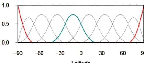
As can be seen from Fig. 2, B-splines are characterized by their compact support or – in other words – they are different from zero only within a small subinterval of length1J1≈ 3·hJ1, where

hJ1= 180◦

2J1+1 (22)

refers to the approximate distance between two consecutive B-splines along the meridian. As the total numberKJ1 of B-splines depends on the levelJ1, finer structures can be mod-eled by increasingJ1. The numerical value for the levelJ1 depends on the global average value1ϕ for the input data sampling interval in the latitudinal direction according to

Figure 2.Polynomial B-splines of levelJ1=3 with a total number KJ1=2

3_{+2=10 of B-splines along the meridian. The blue spline}

functionN_3,42 (ϕ)corresponds to the shift valuek1=4 and covers

a subinterval of length13≈3·180◦/9=60◦. The red spline

func-tionsN_3,02 (ϕ)with shift valuek1=0 andN3,92 (ϕ)with shift value k1=9 close the modeling interval at the poles.

(Schmidt et al., 2011). Solving Eq. (23), considering the level valueJ1from Eq. (22), the inequality

J1≤log2 ₁₈₀◦

1ϕ −1

(24) results.

2.2.2 Trigonometric B-splines

For modeling the longitudinal variations of VTEC trigono-metric B-splinesT_J3

2,k2(λ)of order 3 and, depending on the resolution level, J2∈N0 and shift k2=0, 1, . . . , KJ2−1 are applied. As can be seen from Fig. 3, the total number

KJ2=3·2

J2_{of trigonometric B-splines are located along the} parallels of the chosen spherical coordinate system within the interval λ∈(0◦,360◦). Consequently, the first and the last two B-spline functions within the interval (0◦_,360◦_)have

to be completed by the so-called “wrapping around” effect. This constraint allows trigonometric B-splines to be defined in two different ways:

1. Following Schumaker and Traas (1991), Jekeli (2005) and Limberger (2015) periodic trigonometric B-splines can be calculated by means of a recurrence relation sim-ilar to Eq. (21). Thereby, additional constraints have to be introduced to force the periodicity of the series coef-ficients.

2. The second option was introduced by Lyche and Schu-maker (2001) and used by Schmidt et al. (2011) and Schmidt (2015b). It will be described in the following in more detail.

To be more specific, the sequence of nondecreasing knot points

0◦=λJ2₀ < λJ2₁ < . . . < λJ2_k2 < . . . < λJ2_KJ

2−1<

360◦, (25) with additional knots

λJ2_K

J2+i

=λJ2_i +360◦ for i=0,1,2 (26)

for considering the periodicity is introduced. Similar to the polynomial B-splines, the distance between consecutive knotsλJ2_k2 andλJ2_k2+1fork2=0, 1, . . . ,KJ2+1 is given as

hJ2= 360◦

KJ2

=120

◦

2J2

; (27)

thus, the length of the nonzero subinterval of a trigonometric B-spline functionT_J3

2,k2(λ)reads1J2=3·hJ2=360

◦_/2J2_. Following Lyche and Schumaker (2001) we define the func-tions

MJ2,k2(λ)=T 3

J2,k2(λ)=T 3 hJ₂(λ−λ

J2

k2) . (28) SettinghJ2=handλ−λJk22=2for the sake of simplifica-tion, the functionsT_hJ3

2

(λ−λJ2 k2)=T

3

h(2)can be calculated via

T_h3(2)=

          

         

sin2(2/2)

sin(h/2)sin(h) for 0≤2 < h 1

cos(h/2)−

sin2((2−h)/2)+sin2((2h−2)/2) sin(h/2)sin(h)

for h≤2 <2h sin2((3h−2)/2)

sin(h/2)sin(h) for 2h≤2 <3h 0 otherwise.

(29)

Finally, we define the basis functions

e φJ2

k2(λ)=  



MJ2,k2(λ) for k2=0, . . ., KJ2−3

MJ2,k2(λ)+MJ2,k2(λ−360◦)

for k2=KJ2−2, KJ2−1 (30)

introduced in Eq. (14). Figure 3 shows trigonometric B-splines of level J2=2. With larger values for level J2 the splines become more narrow and finer structures can be mod-eled. The choice of the level valueJ2again depends on the input data sampling interval. Analog to Eq. (23), the inequal-ity

1λ < hJ2 (31)

has to be fulfilled, where1λdenotes the global average value of the data sampling interval in the longitudinal direction. Finally, taking Eq. (27) into consideration, the inequality

J2≤log2 ₁₂₀◦

1λ

(32) for the level valueJ2is obtained.

2.3 Spectral resolution of global VTEC models

In Sect. 2.1 we derived the relations between the maximum degreenmax of a SH expansion and the sampling intervals

Figure 3.K_J2=3·22=12 trigonometric B-splineseφ

J2

k2(λ),

accord-ing to Eq. (30) for levelJ2=2. The blue spline functioneφ2₅(λ)with

shift valuek2=5 is different from zero only in the subinterval of

length1J2=360◦/4≈90◦. The red basis functioneφ₁₁2(λ)shows

the “wrapping-around” effect.

The substitution of the expression 180◦/nmax from the in-equalities Eq. (12) into Eqs. (24) and (32) yields a total of six inequalities

J1≤log2 180◦

1ϕ −1

≤log₂(nmax−1) ,

J2≤log2 120◦

1λ

≤log₂2·nmax 3

. (33)

Given the numerical values 1 to 6 for the B-spline levelsJ1 andJ2Table 1 presents the corresponding largest numerical values for each, the SH degreenmaxand the sampling inter-vals1ϕand1λby evaluating the inequalities using Eq. (33). From the spectral point of view the six inequalities from Eq. (33) comprise the following three scenarios:

1. If the global sampling intervals1ϕand1λare known, the mid parts of the inequalities from Eq. (33) are given. The maximum degreenmaxis calculable from the right-hand side inequalities and may be inserted into the SH expansion in Eq. (10). The left-hand side inequalities yield the two level values J1andJ2which can be in-serted into the B-spline expansion from Eq. (13). 2. With a specified numerical value fornmaxthe right-hand

parts of the inequalities from Eq. (33) are given. The data input sampling intervals1ϕand1λcan be deter-mined from the mid parts of the inequalities. Next, the two numerical values for the level valuesJ1andJ2can be calculated from the left-hand side inequalities and can be inserted into the B-spline expansion in Eq. (13). 3. If the processing time of VTEC maps has to be

consid-ered, the level values J1 andJ2 are subject to certain restrictions; this is due to the fact that the number of numerical operations increases exponentially with the chosen numerical values for the levels. In this case, from the given left-hand side inequalities, the data sampling intervals1ϕ and1λcan be determined from the mid parts. Finally, the right-hand side inequalities yield nu-merical values for the maximum SH degreenmax.

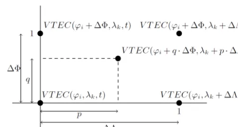
Figure 4.Schematic representation of the four-point spatial interpo-lation to calculate the VTEC value atP (ϕi+q·18, λk+p·13)

from the four corner points of the grid cell of interest.

As already mentioned in the introduction, most of the GIMs produced by the IAACs are based on series expan-sions in SHs up to a maximum degree ofnmax=15. Fol-lowing the abovementioned second strategy and Table 1, we obtain the approximationsJ1=4 (fornmax=17) andJ2=3 (fornmax=12) for the two B-spline levelsJ1andJ2for this example. Inserting these numbers into the B-spline expan-sion Eq. (13) yields the spectrally closest representation to the current IGS solutions. A numerical verification of this choice will be presented in Sect. 4.3.

2.4 VTEC output grids

The VTEC GIMs of the IAACs are usually provided with a spatial resolution of18=2.5◦_{in the latitudinal direction}

and13=5◦_{in the longitudinal direction as well as a}

tempo-ral sampling of1T =2 h. Note, the resolution intervals18,

13and1T are usually distinct from the sampling intervals

1ϕ,1λand1tof the observations introduced in Sect. 2.1. In order to calculate a VTEC value VTEC(ϕ, λ, t )at an arbitrary locationP (ϕ=ϕi+q·18, λ=λk+p·13)with 0≤q≤1 and 0≤p≤1 at an arbitrary time moment t, a simple bilinear spatial interpolation from the VTEC values of the four given corner pointsP (ϕi, λk),P (ϕi, λk+13),

P (ϕi+18, λk)andP (ϕi+18, λk+13)is performed ac-cording to

VTEC(ϕi+q·18, λk+p·13, t )

=(1−q)·(1−p)·VTEC(ϕi, λk, t )

+ q·(1−p)·VTEC(ϕi+18, λk, t )

+ p·(1−q)·VTEC(ϕi, λk+13, t )

+ q·p·VTEC(ϕi+18, λk+13, t ) (34) (see, e.g., Schaer et al., 1998, Fig. 4 in this paper).

Table 1.Numerical values for the B-spline levelsJ1andJ2, the maximum SH degreenmaxand the input data sampling intervals1ϕand1λ

by evaluating the inequalities from Eq. (33); the left part of the table presents the numbers along a meridian (upper inequalities in Eq. 33), and the right part represents the corresponding numbers along the Equator and its parallels according to the lower inequalities in Eq. (33).

Latitude Longitude

J1 1 2 3 4 5 6 J2 1 2 3 4 5 6

nmax 3 5 9 17 33 63 nmax 3 6 12 24 48 96

1ϕ 60 36 20 10.5 5.45 2.85 1λ 60 30 15 7.5 3.75 1.875

1. the chosen model approach, e.g., the SH or the B-spline expansion can be used directly to calculate VTEC val-ues at any arbitrary pointP (ϕ, λ);

2. the resolution intervals18and13of the output grid can be set to smaller values, e.g., to 1◦, as was proposed at the IGS workshop 2012.

For the calculation of a VTEC value VTEC(ϕ, λ, t )at an arbitrary time moment t=ts+r·1T with 0≤r≤1 at a given spatial locationP (ϕ, λ), an interpolation with respect to time can be applied. Commonly, the linear interpolation

VTEC(ϕ, λ, t )=(1−r)·VTEC(ϕ, λ, ts)

+r·VTEC(ϕ, λ, ts+1T ) (35)

between the two consecutive maps at epochsts andts+1T is performed (see, e.g., Schaer et al., 1998).

The previously described interpolation methods allow for the calculation of VTEC values VTEC(ϕ, λ, t )at any spatial locationP (ϕ, λ)and at any timet. However, for a more ac-curate calculation of VTEC an increase in the resolution is necessary for both domains. In the following, it is shown that the usage of a MSR based on the B-spline approach in com-bination with a KF estimation procedure provides the possi-bility to create VTEC maps of higher spatial and temporal resolution. Consequently, according to Table 1 the calculated VTEC maps cover a wider spectral band, i.e., the numerical value ofnmaxbecomes larger.

3 Multi-scale representation

The B-spline functions as introduced in Sect. 2.2.1 and 2.2.2 allow for the generation of a MSR. To be more specific, B-spline tensor product wavelet functions will be constructed which are intrinsically connected to the resolution levels of the MSR. Usually the MSR is interpreted as viewing a sig-nal under different resolutions, as a microscope does (see, e.g., Schmidt, 2012; Schmidt et al., 2015a; Schmidt, 2015b; Liang, 2017). In all of the aforementioned studies, the MSR is based on a regional 2-D representation of VTEC in terms of tensor products of polynomial B-spline functions only. Within this study, however, we apply the MSR for a global 2-D representation of VTEC in terms of tensor products

of polynomial and trigonometric B-spline functions, as de-scribed by Lyche and Schumaker (2001) and Schumaker and Traas (1991).

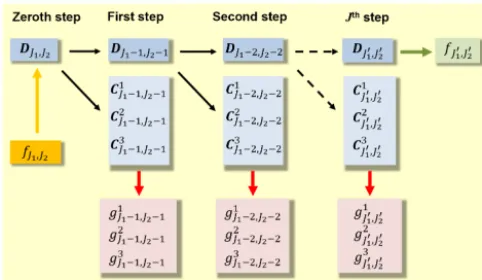
3.1 Pyramid algorithm

Neglecting the time dependency, the B-spline approach Eq. (18) reads

fJ1,J2(ϕ, λ)=φTJ1(ϕ)DJ1,J2eφ_J2(λ) . (36) In the context of the MSR the vectorsφ_J1(ϕ)andeφ_J2(λ) are called scaling vectors, and the elementsd_k1,k2J1,J2 of the ma-trixDJ1,J2are denoted as scaling coefficients.

WithJ₁0=J1−J, J₂0=J2−Jand 0< J≤min(J1, J2)we obtain the 2-D MSR of the target functionf (x)introduced in Eq. (7) as

fJ1,J2(ϕ, λ)=fJ₁0,J₂0(ϕ, λ)+ J X

j=1 3 X

ϑ=1

gϑ_J

1−j,J2−j(ϕ, λ) . (37) Following the argumentation of Schmidt et al. (2015a) but considering the polynomial and the trigonometric B-spline functions the low-passed-filtered level(J₁0, J₂0)signal

f_J0

1,J

0

2(ϕ, λ)and the band-pass-filtered level(J1−j, J2−j ) detail signalsg_J1ϑ_−j,J2−j(ϕ, λ)can be computed via the fol-lowing relations:

f_J0

1,J

0

2(ϕ, λ)=φ T

J₁0(ϕ)DJ₁0,J₂0eφ_J0 2(λ),

g_j1

1−1,j2−1(ϕ, λ)=φ T

j1−1(ϕ)C 1

j1−1,j2−1eψj2−1(λ),

g_j12_−1,j2−1(ϕ, λ)=ψT_j1−1(ϕ)C2_{j1−1,j2−1}eφ_j2−1(λ),

g_j3

1−1,j2−1(ϕ, λ)=ψ T

j1−1(ϕ)C 3

j1−1,j2−1eψj2−1(λ), (38) where we introduced the definitions j1=J1−j+1 and

j2=J2−j+1 forj=1, . . ., J. Herein, theKj1−1×1 and

Kj2−1×1 scaling vectorsφj1−1(ϕ)andeφ_j2−1(ϕ)as well as theLj1−1×1 andLj2−1×1 wavelet vectorsψj1−1(ϕ) and e

ψ_j2−1(λ)can be calculated by means of the two-scale rela-tions

φT_j1−1(ϕ)=φT_j

1(ϕ)Pj1, eφ

T

j2−1(λ)=eφ T

j2(λ)ePj2,

ψT_j

1−1(ϕ)=φ T

j1(ϕ)Qj1, e

ψT_j

2−1(λ)=eφ T

Figure 5.A 2-D MSR of the signalfJ1,J2(ϕ, λ).

withLj1−1=Kj1−Kj1−1andLj2 =Kj2−Kj2−1.

The numerical entries of theKj1×Kj1−1matrixPj1 and theKj1×Lj1−1matrixQj1can be taken from Stollnitz et al. (1995b) or Zeilhofer (2008); the corresponding entries of the

Kj2×Kj2−1matrixePj2 and theKj2×Lj2−1matrixQe_j 2 are provided by Lyche and Schumaker (2001).

In Eq. (38) we introduced the Kj1−1×Kj2−1 matrix Dj1−1,j2−1of scaling coefficients d

j1−1,j2−1

k1,k2 as well as the

Kj1−1×Lj2−1 matrix C1_j

1−1,j2−1, the Lj1−1×Kj2−1 ma-trixC2_j

1−1,j2−1and theLj1−1×Lj2−1matrixC 3

j1−1,j2−1of wavelet coefficients. These four matrices can be calculated via the 2-D downsampling equation

"

Dj1−1,j2−1 C1_j 1−1,j2−1 C2_{j1−1,j2−1} C3_{j1−1,j2−1} #

=

Pj1

Q_j

1

Dj1,j2 h

e PT_j

2 Qe T j2 i

,

(40)

also known as the 2-D pyramid algorithm. TheKj1−1×Kj1 matrix Pj1, theKj2−1×Kj2 matrix ePj2, the Lj1−1×Kj1 matrixQ_j1 and theLj2−1×Kj2matrixQej2can be computed via the identities

_P

j1

Q_j1

= _P

j1 Qj1 −1

, (41)

" e Pj2

e Q_j2

#

= ePj2 Qe_j 2

−1

(42)

(see, e.g., Schmidt, 2007). The 2-D pyramid algorithm based on the decomposition Eq. (37) is visualized in Fig. 5. The “zeroth” step transforms the observationsy(xij, tj) accord-ing to Eqs. (13) and (18) into the elements of the scalaccord-ing matrix DJ1,J2(tj)as introduced in Eq. (17). The procedure applied will be explained in Sect. 3.2.

The previously described MSR refers to a successive low-pass filtering of the target functionf (ϕ, λ, t )into two direc-tions, namely latitudeϕand longitudeλ, in the same manner. If a signalf (ϕ, λ, t )is represented according to Eq. (18) up

Figure 6.A 1-D MSR of the signalfJ1,J2(ϕ, λ)with respect to the

latitudeϕ. The “zeroth” step on the left-hand side conforms with the one in Fig. 5.

to the level values J1 with respect to latitude and J2 with respect to longitude, i.e.,f (ϕ, λ, t )≈fJ1,J2(ϕ, λ, t ), the ap-plication of the MSR Eq. (37) allows for the computation of low-pass-filtered signal approximations up to the level pairs

(J1−1, J2−1),(J1−2, J2−2),. . .. The principal structures of the ionospheric key parameters such as VTEC, however, are usually parallel to the geomagnetic Equator. Consequently, we will additionally deal with a 1-D MSR of the signal

f (ϕ, λ, t )with respect to the latitude. In this case Eq. (37) reduces to

fJ1,J2(ϕ, λ)=fJ₁0,J2(ϕ, λ)+ J X

j=1

gJ1−j,J2(ϕ, λ). (43)

Thus, signal approximations up to the level pairs(J1−1, J2),

(J1−2, J2), . . . are obtained. From the four relations in Eq. (38) only the first and the third one have to be consid-ered within the 1-D MSR Eq. (43), namely

f_J0

1,J2(ϕ, λ)=φ T

J₁0(ϕ)DJ₁0,J2eφ_J2(λ), gj1−1,J2(ϕ, λ)=ψ

T

j1−1(ϕ)C 2

j1−1,J2eφJ2(λ) (44) withj1=J1−j+1 forj=1, . . ., J, 0< J≤J1 andJ₁0=

J1−J. TheKj1−1×KJ2 matrixDj1−1,J2 of scaling coeffi-cients and theLj1−1×KJ2 matrixC2_j1−1,J2 of wavelet coef-ficients can be calculated from the 1-D downsampling equa-tion

_D

j1−1,J2 C2_j

1−1,J2

=

Pj1 Qj1

Dj1,J2, (45)

where the matrices Pj1 and Qj1 can be computed via Eq. (41). The 1-D pyramid algorithm based on the decom-position Eq. (43) is visualized in Fig. 6.

3.2 Estimation of unknown model parameters

To estimate the elements of the unknown KJ1×KJ2 ma-trixDJ1,J2(ts)from VTEC observationsy(xis, ts)(cf. Eq. 8) within the “zeroth” step of the MSR we apply Kalman filter-ing accordfilter-ing to Erdogan et al. (2017).

In the linear formulation the Kalman filter consists (1) of the state equation

β_s=Fsβs−1+ws−1 (46) and (2) of the system

y_s+es=As βs (47)

of observation equations. In Eq. (46 ) theu×1 vectorβ_s=

vecDJ₁,J2(ts) – known as the state vector – of the u =

KJ1·KJ2 unknown scaling coefficients at time moment ts is predicted from the state vectorβ_s−1of the previous time moment ts−1 by means of the u×u transition matrix Fs and theu×1 vectorws−1of the process noise. In Eq. (47)

y_s =(y(xis, ts))andes=(e(xis, ts))are theIs×1 vectors of the observations and the measurement errors, respectively; the(is)th row vectoraT_is of theIs×ucoefficient matrixAsis given by the expression

ais =eφJ2(λis) ⊗ φJ1(ϕis), (48) as introduced in Eq. (18). The measurement error vectores and the vector ws of the process noise are assumed to be white noise vectors with expectation values E(es)=0 and

E(w_s)=0, and fulfill the requirements

E(w_swT_l )=6wδs,l, E(eseTl )=6yδs,l,

E(wseTl )=0, (49)

whereδs,lis the delta symbol that equals 1 fors=land 0 for

s6=l. In Eq. (49)6yand6w are given covariance matrices of the observations and the process noise, respectively.

The solution of the estimation problem as defined in Eqs. (46) and (47) generally consists of the sequential ap-plication of a prediction step (time update) and a cor-rection step (measurement update). In the prediction step, the estimated state vector bβ_s−1 and its covariance matrix

b

D(bβ_s−1)=b6β,s−1 are propagated from the time moment

ts−1to the next time momenttsby means of

β−_s =Fsbβ_s−1, (50)

6−_β,s=Fs b6β,s−1FTs +6w, (51) where the symbol “–” indicates the predicted quantities. The prediction step is followed by the measurement update

b

β_s=β−_s +Ks (ys−As β−s) , (52) b

6β,s=(I−Ks As)6−_β,s, (53) wherebβ_s andb6β,s are the updated state vector and its co-variance matrix, respectively. In Eqs. (52) and (53) theu×Is

Kalman gain matrix

Ks=6−_β,sATs (As 6−_β,sATs +6y)−1 (54) behaves as a weighting factor between the new measure-ments and the predicted state vector. The chosen step size

ts − ts−1within the KF determines the maximum temporal resolution of the output.

Using the estimationsbβ_sand6bβ,sfrom Eqs. (52) and (53), aV×1 vectorf_s of function valuesf (ϕi, λk, ts)at arbitrary locationsP (ϕi, λk)withi=1, . . . ,I,k=1, . . . ,KandV =

I·Kcan be estimated by b

f_s=Asbβ_s, (55)

b 6f,s =A

T

s 6bβ,sAs , (56) where6bf,s is the estimatedV ×V covariance matrix of the estimation bf_s. The V×u matrix As is set up in a simi-lar way to matrixAs in Eq. (47) with Eq. (48). In the fol-lowing, we will interpret the function valuesf (ϕi, λk, ts)= VTEC(ϕi, λk, ts)as VTEC values.

3.3 B-Spline model output

The previously explained procedure allows for the dissemi-nation of two products to the users:

– Product 1:a set of estimated scaling coefficients b

dJ1,J2 k1,k2(ts)

k1=0,...,KJ

1−1,k2=0,...,KJ2−1

(57) from Eq. (52) at time momentstsfor level valuesJ1and

J2at the spatial positionsk1in the latitudinal direction andk2in the longitudinal direction, respectively, as well as their estimated standard deviations

bσ J1,J2 d;k1,k2(ts)

k1=0,...,KJ₁−1,k2=0,...,KJ₂−1 (58) extracted from the covariance matrix Eq. (53).

– Product 2:estimated VTEC values given as \

VTECJ1,J2(ϕi, λk, ts)

_{i=1,...,I,k=1,...,K} (59) according to Eq. (55) at time momentstsfor level values

J1 andJ2 in the latitudinal and longitudinal direction, respectively, calculated at grid pointsP (ϕi, λk)as well as their estimated standard deviations

bσ J1,J2

VTEC(ϕi, λk, ts)

i=1,...,I,k=1,...,K, (60) extracted from the covariance matrix Eq. (56).

Following Eq. (34), the coordinatesϕiandλkof all of theV grid pointsP (ϕi, λk)are defined asϕi= −90◦+(i−1)·18 with 18=180◦_{/(I−1) and λ}

k=0◦+(k−1)·13 with

13=360◦/K. As previously mentioned, the spatial reso-lution intervals18and13are usually chosen as 1◦, 2.5◦ or 5◦, i.e.,I=181, 73, 37 andK=360, 144, 72.

The two products, i.e., the set of coefficients or the VTEC grid values reflect the two strategies of dissemination. In case of a SH expansion for RT applications as introduced in Sect. 2.1 the corresponding SH coefficients cn,m from Eq. (10) can be transferred to the user by means of a RTCM (Radio Technical Commission for Maritime services) stan-dard 1264 message. This message allows for the considera-tion of SH coefficients, but only up to degreen=16. In the case of the B-spline expansion Eq. (13), however, an encoder procedure for the B-spline coefficients Eq. (57) is necessary, because the user has to evaluate the B-spline model just as in the SH case by substituting the B-spline tensor product Eq. (14) for the SHs Eq. (11). Due to the two restrictions, namely the sole use SH expansions and only up to a maxi-mum degreenmax=16, the RTCM message format for data dissemination has to be urgently discussed and must be set up in a more flexible way (refer to the comments in Sect. 5). To apply the RTCM format in its current form, the VTEC grid values Eq. (59) can alternatively be used as observations

y(xis, ts)in Eq. (10) to calculate SH coefficientscn,m(ts)by means of a least-squares estimation. This way each GIM can be sent at a high update rate to the user for RT applications.

For Product 2, the VTEC grid values Eq. (59) as well as there standard deviations Eq. (60) are disseminated as VTEC and standard deviation maps, i.e., GIMs, with given spatial resolutions18and13 in the latitudinal and longitudinal direction, respectively, in IONEX format to the user.

4 Numerical investigations

In the following, the described modeling approach developed at DGFI-TUM is applied to real data. To be more specific, we use GPS and GLONASS NRT data in hourly blocks and apply ultra-rapid orbits. A detailed explanation of the data preprocessing and the setup of the full observation equations is presented by Erdogan et al. (2017). The IGS IAACs pro-vide final products based on post-processed GNSS observa-tions and orbits with a latency of more than 1 week. Several IAACs additionally provide rapid products with a latency of 1 d using rapid orbits. An overview on the products used in the this paper is given in Table 2.

For the evaluation of the data we have to define an appriate coordinate system. Here we follow the standard pro-cedure and use a sun-fixed geomagnetic coordinate system. To be more specific, we identify the coordinate system 6E introduced in the context of Eq. (3) with the Geocentric So-lar Magnetic (GSM) coordinate system (see, e.g., Laundal and Richmond, 2017). Consequently, the SH and B-spline

Table 2.List of GIM products used in this paper. Information on names, types and latencies are taken from the following references: (1) Roma-Dollase et al. (2017), (2) Orus et al. (2005) and (3) this paper.

Institution Product Type Latency Reference CODE codg Final >1 week (1) UPC uqrg Rapid >1 d (2) DGFI- oplg

TUM ophg NRT <3 h (3)

theory as presented in the previous sections is applied in the orthogonal GSM system. As diurnal variations of the iono-sphere are mitigated in this coordinate system, the transition matrixFs introduced in the state Eq. (46) of the KF can be set to the identity matrixI, i.e.,Fs=I. In other words, the dynamic system of the KF is set to a random walk process. Furthermore, for the time update in Eq. (46) we fix the step sizets−ts−1to 5 min.

While the scaling coefficients Eq. (57) and their standard deviations Eq. (58) of Product 1 are located within the GSM system, the VTEC values Eq. (59) and their standard devi-ations Eq. (60) of Product 2 are provided in the aforemen-tioned IONEX format on a regular grid defined in a geo-graphical geocentric Earth-fixed coordinate system. Thus, a coordinate system transformation has to be interposed. 4.1 Validation procedure

For validation purposes we rely on the dSTEC analysis which is currently regarded as the standard method for the qual-ity assessment of VTEC models (see, e.g., Orus et al., 2007; Rovira-Garcia et al., 2015).

This analysis method is based on the calculation of the difference between STEC observations STEC(xS,xR, ts)at discrete time momentstsaccording to Eq. (2) and a reference observation STEC(xS_,x

R, tref)along a specified satellite arc as

dSTECobs(ts)=STEC(xS,xR, ts)

−STEC(xS,xR, tref) . (61) The reference time momentt=trefis usually referred to the observation with the smallest zenith angle z=zref. In the same manner, the differences

dSTECmap(ts)=M(zs)·VTEC(xIPP, ts)

−M(zref)·VTEC(xIPP,tref) (62) are calculated by means of Eq. (5) from the VTEC map to be validated. The quality assessment is performed by studying the differences

Figure 7.Global distribution of the IPPs from GPS (red dots) and GLONASS (blue stars) measurements for 6 September 2017, at 13:00 UT.

4.2 Estimation of B-spline multi-scale products

Figure 7 shows the global distribution of the IPPs related to GNSS VTEC observations y(xIPP, ts)=VTEC(xIPP, ts)as introduced in Eq. (13) for 6 September 2017 at 13:00 UT. As the B-spline model is set up in the GSM coordinate system and the scaling coefficients are restricted to the state equation

d_k1,k2J1,J2(ts)=d_k1,k2J1,J2(ts−1)+w(ts−1) (64) according to Eq. (46), we select1ϕ=5◦_and1λ=10◦_as

appropriate values for the global average sampling interval of the input data as introduced at the end of Sect. 2.1. Con-sequently, the B-spline levels toJ1=5 andJ2=3 are taken from Table 1.

The covariance matrices 6y and6w of the observations and the process noise, respectively, as defined in the formu-lae of Eq.(49), are set up according to Erdogan et al. (2017). In more detail, 6y consists of two diagonal block matrices related to GPS and GLONASS VTEC observations. The rel-ative weighting between the blocks, i.e., between GPS and GLONASS, is performed by manually defined variance fac-tors.

Figure 8a shows withJ1=5, J2=3,KJ1=2

J1₊₂₌₃₄ and KJ2=3·2

J2 _{=24, the numerical values of the total} 816=34·24 scaling coefficients are

b d_k1,k25,3(ts)

k1=0,...,33, k2=0,...,23 (65) according to Eq. (57), estimated by means of Eq. (52). As the shift values k1andk2determine the location of the scaling coefficients, they can be plotted. Figure 8b shows the corre-sponding standard deviations as defined in Eq. (58). A test of significance is performed for each of the scaling coefficients according to Koch (1999).

While Fig. 8a and b show the results of Product 1 in the GSM system, Fig. 8c and d depict the corresponding results of Product 2 in a geographical geocentric coordinate sys-tem. With the choices18=2.5◦and13=5.0◦for the grid spacing in the latitudinal and longitudinal directions, respec-tively, Product 2 provides the VTEC grid values

\

VTEC5,3(ϕi, λk, ts)

_{i=1,...,73,k=1,...,72} (66)

and the corresponding standard deviations _bσ_VTEC5,3 from Eqs. (59) and (60).

Note that for the visualization of VTEC and their standard deviations in Fig. 8c and d, we computed function values on a much denser grid using the interpolation formula (34).

From the comparison of Fig. 8a and c, it can be stated that the numerical values of the scaling coefficients directly re-flect the signal structure, i.e., the signal energy. This fact is the consequence of the localizing character of the B-spline functions. Figure 8b and d reveal that the standard devia-tions are generally larger where no or only a few GNSS ob-servations from IGS stations are available, namely over the oceans, e.g., the Southern Atlantic, but also over specific con-tinental regions such as the Sahara and the Amazon region.

Figure 8a, i.e., the plot of the set of scaling coefficients b

d_k15,3_,k2 in Eq. (65) can be interpreted as a visualization of the 34×24 matrixD5,3defined in Eq. (17) and displayed in the top-left boxes of Figs. 5 and 6 for the 2-D and the 1-D MSR, respectively. Consequently, Fig. 8a and b are the results of the zeroth step within the pyramid algorithm, as explained in Sect. 3. Applying the first step of the 1-D pyramid algorithm, the downsampling Eq. (44) provides both the 18×24 matrix D4,3of estimated scaling coefficientsbd

4,3

k1,k2 for the level val-uesJ1=4 andJ2=3 as well as the 16×24 matrixC2_4,3of estimated wavelet coefficients. Consequently, the definition of Product 2 in Sect. 3.3 can be extended to“Multi-Scale Products 2”:

– ophg:estimations with levelsJ1=5,J2=3

\

VTEC5,3(ϕi, λk, ts), bσ 5,3

VTEC(ϕi, λk, ts)

18=2.5◦, 13=5.0◦; (67)

– oplg:estimations with levelsJ1=4,J2=3

\

VTEC4,3(ϕi, λk, ts), bσ 4,3

VTEC(ϕi, λk, ts) bg4,3(ϕi, λk, ts), bσ

4,3

g (ϕi, λk, ts)

18=2.5◦, 13=5.0◦. (68)

We denote the two Multi-Scale Products 2 as “ophg” and “oplg”’, where the first symbols refer to the OPTIMAP pro-cessing software, which was developed within a third-party funded project (see Acknowledgements). The “p” is cho-sen according to the temporal output sampling1T of maps, with “t” for 1T =10 min, “1” for 1T =1 h and “2” for

Figure 8.Estimated scaling coefficients(a)and their standard deviations(b)for level valuesJ1=5 andJ2=3 within the GSM coordinate

system. Estimated VTEC values(c)and their standard deviations(d)as GIMs within a geographical coordinate system; all sets calculated for 6 September 2017 at 13:00 UT.

4.3 Comparison of VTEC maps from B-spline and spherical harmonic expansions

As mentioned in the context of Table 1, the B-spline levels

J1=4 for latitude andJ2=3 for longitude fit best to the highest degree nmax=15 of a SH expansion Eq. (10). To be more specific, we compare the multi-scale product “o1lg” with the product “codg” provided by CODE. “codg” is char-acterized by a SH expansion up to degree nmax=15 and a time interval 1T =1 h of two consecutive maps (Schaer, 1999).

Figure 9 shows the VTEC and standard deviation maps for 6 September 2017 at 13:00 UT as well as the difference map between “o1lg” and “codg”. Although the structures of the two VTEC maps are rather similar, the difference map shows deviations of up to±6 TECU. To judge this amount, a comparison of VTEC GIMs from different IAACs was per-formed (not shown here). This investigation stated that devi-ations between individual IAAC products can reach±10 % or even more. Studying the structures within the difference map no larger systematic patterns are visible and, thus, jus-tify our assumption that the quality of “o1lg” is comparable with the quality of the IAAC products. The standard devia-tion maps in Fig. 9b and d show different structures that are mainly caused by the application of the different estimation strategies, namely KF (“o1lg”) and least-squares estimation (“codg”).

To numerically assess the comparability we apply the dSTEC analysis described in Sect. 4.1. First we define a net-work of receiver stations which are used in Eq. (61).

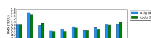
The chosen set should not be used within the computation of the VTEC maps. Fulfilling both requirements at the same time is difficult and, thus, the set of stations shown in Fig. 10 contains both independent stations and stations used simul-taneously in all VTEC models. As GNSS measurements are taken along the satellite arcs, the corresponding IPPs are lo-cated spatially within a grid cell and temporally between the discrete time moments of the “o1lg” and “codg” products. In order to calculate the VTEC values in Eq. (62), the spatial and temporal interpolation formulae (34) and (35) have to be applied. Figure 11 shows the RMS values of the differences Eq. (63) during the time span between 1 and 30 Septem-ber 2017, at the chosen receiver stations.

As can be seen, the RMS values vary between 0.3 and 1.6 TECU. By comparing the RMS values of “o1lg” with a mean RMS value of 0.80 TECU and “codg” with a mean RMS of 0.77 TECU we can state that the quality of these two products is very close to each other.

Figure 9.VTEC maps “codg”(a)and “o1lg”(c)as well as their standard deviation maps(b, d); difference map of the two VTEC maps(e); all data for 6 September 2017 at 13:00 UT.

Figure 10.Distribution of the 10 IGS receiver stations used for the dSTEC analysis.

(68). In what follows, we study them during a solar storm of medium intensity on 8 September 2017 and during the strongest storm of the last 10 years, the prominent St. Patrick storm, which occurred on 17 March 2015. Figure 12a, c, and d show the results of the 8 September 2017 event at 19:00 UT

Figure 11.RMS values for the “codg” (green) and “o1lg” (blue) products computed at the 10 receiver stations shown in Fig. 10. The values in parentheses in the legend are the average RMS values over all 10 receiver stations for the entire test period between 1 and 30 September 2017.

and Fig. 12b, d, and e display the corresponding maps for the St. Patrick storm event on 17 March 2015 at 19:00 UT.

As already mentioned in the context of Eq. (43), it is ex-pected that the detail signal Eq. (44) is dominated by struc-tures parallel to the geomagnetic Equator. The detail signal

Figure 12. Multi-scale VTEC products for solar storm events: high-resolution VTEC map “ophg” for 8 September 2017(a)and for 17 March 2015(b); low-resolution VTEC map “oplg” for 8 September 2017(c)and for 17 March 2015(d); panels(e)and(f)show the detail signals introduced in equation block Eq. (68) and computed by means of Eq. (44) for the two solar events.

a large number of estimated wavelet coefficients collected in the matrixC_4,32 are characterized by absolute values smaller than a given threshold. The neglect of these coefficients al-lows for a high data compression rate. Consequently, the number of significant coefficients as the outcome of a MSR would go drastically below the number of scaling coefficients within the set Eq. (57) of Product 1; the reader can get an im-pression of the number of neglected coefficients by paying attention to the light green and light blue colors in Fig. 12e and f. This advantageous feature of the MSR was not stud-ied within this work but will be applstud-ied and published in the future.

Next, we focus on the solar storm during September 2017 and study the temporal sampling intervals of different GIMs. In summary, we distinguish between six products of different spectral content and different sampling intervals.

Figure 13 depicts the RMS values computed by the dSTEC analysis at the stations shown in Fig. 10. It is assumed that a product with a larger sampling interval 1T is less accu-rate than a product with a smaller sampling interval.

Conse-Figure 13.RMS values for the “o2hg”, “o1hg”, “othg”, “o2lg”, “o1lg” and “otlg” products computed at the 10 receiver stations shown in Fig. 10 during September 2017. The values in parentheses in the legend are the average RMS values over all 10 receiver sta-tions for the entire test period between 1 and 30 September 2017.

Table 3.Relative improvements (in percentage) for a downsizing of the sampling interval of the “o2lg”, “o1lg”, “otlg”, “o2hg”, “o1hg” and “otlg” products.

Product RMS [TECU] Percentage Improvement o2lg 0.92 100%

o1lg 0.80 87.0% 13.0% otlg 0.77 83.7% 16.3% o2hg 0.90 100%

o1hg 0.72 80.0% 20.0% othg 0.68 75.6% 24.4%

Table 4.Results (in percentage) of the comparisons of the high-resolution products “ophg” with the low-high-resolution products “oplg”. Positive (bold) numbers mean an improvement, and negative (italic) values represent a reduction in the quality.

o2lg o1lg otlg o2hg 2.2% −12.5% −16.9% o1hg 21.7% 10.0% 6.5% othg 26.1% 15.0% 11.7%

blue (“o1lg”) vs. blue (“o1hg”) and green (“otlg”) vs. yellow (“othg”), the aforementioned assumptions are confirmed.

The differences in the RMS values of the first three prod-ucts, “o2lg”, “o1lg” and “otlg”, are caused by their different sampling intervals. Comparing the mean RMS values of 0.92 and 0.80 TECU for “o2lg” and “o1lg”, respectively, we find a relative improvement of approximately 13.0 %. By decreas-ing the sampldecreas-ing from1T =2 h to1T =10 min, a further improvement of 16.3 % can be achieved.

Comparing the RMS values 0.90, 0.72 and 0.68 TECU of the “o2hg”, “o1hg” and “othg” products, respectively, we find relative improvements of 20 % and 24.4 % by downsiz-ing the sampldownsiz-ing interval from 2 to 1 h and finally to 10 min. A summary of the relative improvements is given in Table 3. In the next step, we compare the quality of the multi-scale products “ophg” and “oplg” directly. First, we compare “o2lg” with “o2hg” and obtain an improvement of approxi-mately 2.2 % . In the same manner, we compare “o1lg” with “o1hg” and “otlg” with “othg” and find that improvements of 10.0 % and 11.7 % can be achieved, respectively. Table 4 shows the results for the comparison of each pair of products; an improvement is indicated by numbers in bold font, and a deterioration is indicated by numbers in italic font. As a con-sequence, an increase of the numerical value for levelJ1, i.e., the enhancement of the spectral resolution with respect to the latitude yields a significant improvement in the RMS values as long as the temporal sampling1T is less than 2 h.

From the investigations in Sect. 4.3, it could be concluded that the quality of the “o2lg” product is comparable to the quality of the IAAC products. It can be seen from Table 4

Figure 14.RMS values for the “uqrg” and “othg” products com-puted at 9 IGS receiver stations during September 2017. The val-ues in parentheses in the legend are the average RMS valval-ues over all 9 receiver stations for the entire test period between 1 and 30 September 2017.

that there is a strong improvement of more than 26 % when using the “othg” product instead of the “o2lg” product. It is worth mentioning that both products are based on the same input data and are spatially related to each other by means of the MSR.

4.5 Assessment of high-resolution VTEC models As the “othg” product outperforms all other products used in the previous sections we now compare it with UPC’s “uqrg” product (Roma-Dollase et al., 2017) which provides smaller values in the relative standard deviation of their dSTEC anal-ysis in comparison with the products of other IAACs. “uqrg” is a rapid product and is provided with a sampling interval

1T =15 min. As the “NKLG” station is not used in the cal-culation of “uqrg”, it is excluded from the calcal-culation of the overall RMS value shown in the legend.

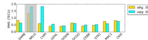
As can be seen, the RMS values vary between 0.5 and 1.8 TECU but are mostly below 1.0 TECU. The dominant RMS value of “uqrg” at the “CHPI” station reduces its qual-ity significantly. If “CHPI” is neglected, the mean RMS value of “uqrg” decrease to 0.59 TECU. Summarizing these inves-tigations, we can state that the overall quality of the two prod-ucts is very similar. Considering the fact that “othg” is a NRT product with a latency of less than 3 h, it also outperforms “uqrg” which is a rapid product with a latency of around 1 d (see Table 2). However, for a final assessment, further val-idation studies have to be performed between the different products.

5 Conclusions and outlook

Figure 15. DGFI-TUM’s processing modules, including (blue boxes) the download and preprocessing module for GNSS obser-vations, the modeling module by means of B-splines, MSR and Kalman filtering (orange boxes) with possible output as Product 1 and Product 2 (yellow boxes) and the validation module.

VTEC maps of the IAACs to rate the quality. As the dSTEC analysis is the most frequently used validation method, we abandon a comparison with satellite altimetry products here. To summarize the validation studies, it can be stated that the high-resolution “othg” product outperforms all products used within the selected time span of investigation.

Besides the facts, that our models can handle data gaps due to the utilization of localizing basis functions, the applica-tion of a KF to include a dynamic predicapplica-tion procedure and the use of the MSR to create products of different spectral content at the same time, it should be mentioned that DGFI-TUM’s products

– are based on NRT GNSS observations only, i.e., are us-ing input data with a latency of less then 3 h (in contrast, “codg” relies on post-processed data with a latency of larger than 3 weeks, and “uqrg” relies on rapid data with a latency of at least 1 d; cf. Table 2);

– rely on specially developed software modules (cf. Fig. 15), e.g., the preprocessing module using ultra-rapid orbits;

– and can be disseminated to users with a delay of 2–3 h. In general, the dissemination of these products to users can be undertaken in two different ways: based on estimated scal-ing coefficients (Product 1) or by calculated VTEC grid val-ues (Product 2). For RT applications, however, the dissemi-nation in terms of Product 1 is preferred, in particular the us-age of the RTCM format. In the scope of the developments in the recent years, RT applications have become more impor-tant, e.g., in unmanned or autonomous vehicle development; thus, the restriction of the RTCM message to allow only for SH coefficients needs to urgently be discussed. Particularly from the point of view that there are also other modeling methods, a modification of the RTCM format would be ap-propriate. The MSR allows for significant data compression to be obtained due the step-wise downsampling of the scal-ing coefficients accordscal-ing to the pyramid algorithm. Details

represented in the signalfJ1,J2 of the zeroth step are stored in wavelet coefficients for the following steps (see Fig. 5). A large number of estimated wavelet coefficients are character-ized by absolute values smaller than a given threshold and, thus, most of them can be neglected for the reconstruction of the original signal. Hence, the overall number of scaling and wavelet coefficients can be reduced drastically. Consid-ering this powerful feature of data compression, we propose replacing the scaling coefficients of the highest levels with the significant wavelet coefficients of the lower levels for a definition of an alternative and more appropriate format for data dissemination in terms of Product 1.

The results presented encourage the further development of high accuracy VTEC maps. By extending the models by a fourth dimension, i.e., modeling of the electron density directly, inaccuracies due to the mapping function can be avoided. To model the vertical structure of the electron den-sity, additional observations have to be incorporated, e.g., from DORIS, satellite altimetry and ionospheric radio occul-tations. This would mitigate the inhomogeneity of the data distribution and, in turn, even higher levels of the B-spline expansion can be chosen.

Data availability. The global VTEC maps in IONEX format used in the comparisons were acquired from the Crustal Dynamics Data Information System (CDDIS) data center by the following FTP server: ftp://cddis.gsfc.nasa.gov/gnss/products/ionex/. The hourly available GNSS data from IGS sites were operationally down-loaded in real time through mirroring to the different IGS data centers, i.e., the CDDIS (ftp://cddis.gsfc.nasa.gov/pub/gps/data/ hourly/), the Bundesamt für Kartographie und Geodäsie (BKG) (ftp://igs.bkg.bund.de/IGS/nrt/), the Institut Geographique National (IGN) (ftp://igs.ensg.ign.fr/pub/igs/data/hourly) and the Korean As-tronomy and Space Science Institute (KASI) (ftp://nfs.kasi.re.kr/). Furthermore, the ultrarapid orbits of GPS and GLONASS satellites utilized in the data preprocessing step can be accessed through FTP servers: for GPS via ftp://cddis.gsfc.nasa.gov/pub/gps/products, and for GLONASS via ftp://ftp.glonass-iac.ru/MCC/PRODUCTS/.

Author contributions. The concept for the paper was proposed by AG and discussed with all co-authors. AG compiled the figures and wrote the paper with assistance from MS. The paper and figures were reviewed by all co-authors.

Competing interests. The authors declare that they have no conflict of interest.