SIP: Optimal Product Selection from Feature Models Using Many-Objective Evolutionary Optimization

(1)

Many-Objective Evolutionary Optimization

.

White Rose Research Online URL for this paper:

http://eprints.whiterose.ac.uk/147601/

Version: Accepted Version

Article:

Hierons, R.M. orcid.org/0000-0002-4771-1446, Li, M., Liu, X. et al. (2 more authors) (2016)

SIP: Optimal Product Selection from Feature Models Using Many-Objective Evolutionary

Optimization. ACM Transactions on Software Engineering and Methodology, 25 (2). 17.

ISSN 1049-331X

https://doi.org/10.1145/2897760

© ACM, 2016. This is the author's version of the work. It is posted here by permission of

ACM for your personal use. Not for redistribution. The definitive version was published in

ACM Transactions on Software Engineering and Methodology, Volume 25 Issue 2, May

2016 http://doi.acm.org/10.1145/2897760

Reuse

Items deposited in White Rose Research Online are protected by copyright, with all rights reserved unless indicated otherwise. They may be downloaded and/or printed for private study, or other acts as permitted by national copyright laws. The publisher or other rights holders may allow further reproduction and re-use of the full text version. This is indicated by the licence information on the White Rose Research Online record for the item.

Takedown

If you consider content in White Rose Research Online to be in breach of UK law, please notify us by

(2)

SIP: Optimal Product Selection from Feature Models using

Many-Objective Evolutionary Optimisation

Robert M. Hierons, Brunel University London, UK

Miqing Li, Brunel University London, UK

XiaoHui Liu, Brunel University London, UK

Sergio Segura, University of Seville, Spain

Wei Zheng, Northwestern Polytechnical University, China

A feature model specifies the sets of features that define valid products in a software product line. Recent work has considered the problem of choosing optimal products from a feature model based on a set of user preferences, with this being represented as a many-objective optimisation problem. This problem has been found to be difficult for a purely search-based approach, leading to classical many-objective optimisation al-gorithms being enhanced by either adding in a valid product as a seed or by introducing additional mutation and replacement operators that use a SAT solver. In this paper we instead enhance the search in two ways: by providing a novel representation and also by optimising first on the number of constraints that hold and only then on the other objectives. In the evaluation we also used feature models with realistic attributes, in contrast to previous work that used randomly generated attribute values. The results of experiments were promising, with the proposed (SIP) method returning valid products with six published feature models and a randomly generated feature model with 10,000 features. For the model with 10,000 features the search took only a few minutes.

CCS Concepts:r_{Software and its engineering}_→_{Software product lines;}r_{Mathematics of} comput-ing→Optimization with randomized search heuristics;

Additional Key Words and Phrases: Product Selection

ACM Reference Format:

Robert M. Hierons, Miqing Li, XiaoHui Liu, Sergio Segura, and Wei Zheng, 2015. SIP: Optimal Product Selection from Feature Models using Many-Objective Evolutionary OptimisationACM Trans. Softw. Eng. Methodol.V, N, Article A (January YYYY), 34 pages.

DOI:http://dx.doi.org/10.1145/0000000.0000000

1. INTRODUCTION

In recent years there has been significant interest insoftware product lines (SPLs)in which families of products are systematically developed using a set of reusable assets. The set of products within an SPL is typically described by a feature model, with a feature being some aspect of system functionality [Clements and Northrop 2001]. A product is seen as being a set of features and the feature model defines the constraints between features and so specifies which combinations of features define valid products. There is evidence of feature models being used by companies such as Boeing [Sharp 1998], Siemens [Hofman et al. 2012], and Toshiba [Matsumoto 2007].

Author addresses: R. M. Hierons, Department of Computer Science, Brunel University London, UK and Miqing Li, Department of Computer Science, Brunel University London, UK and XiaoHui Liu, Department of Computer Science, Brunel University London, UK and Sergio Segura, University of Seville, Spain and Zheng Wei, Northwestern Polytechnical University, China

Permission to make digital or hard copies of all or part of this work for personal or classroom use is granted without fee provided that copies are not made or distributed for profit or commercial advantage and that copies bear this notice and the full citation on the first page. Copyrights for components of this work owned by others than ACM must be honored. Abstracting with credit is permitted. To copy otherwise, or repub-lish, to post on servers or to redistribute to lists, requires prior specific permission and/or a fee. Request permissions from [email protected].

c

YYYY ACM. 1049-331X/YYYY/01-ARTA $15.00

(3)

Much of the focus of research regarding feature models has been on automated tech-niques that analyse a feature model [Benavides et al. 2010]. This has led to a range of techniques that will, for example, determine whether a feature model is valid (defines one or more products) or whether there are features that appear in no valid products. There are tools such as FaMa [Benavides et al. 2007], SPLAR [Mendonca et al. 2009] and FeatureIDE [Th ¨um et al. 2014] that implement many analysis techniques.

Another line of work has considered the problem of automatically determining ‘op-timal’ products based on a feature model and information regarding user preferences. The result of a search might be used, for example, to determine which products to re-lease first or which to test. Naturally, there are several aspects that can be used to determine whether a product is ‘optimal’ and these relate to the values of attributes of the features1_{. For example, one might prefer products that contain many features} since these will satisfy the demands of more customers. One might also favour prod-ucts that have a low associated cost. Recently Sayyad et al. [Sayyad et al. 2013d] noted that this leads to a many-objective optimisation problem2 _{and they explored the use} of several many-objective optimisation algorithms. Since a product must satisfy all of the constraints in the feature model, one objective was the number of constraints that fail. In this initial piece of work they used sixevolutionary many-objective optimisation (EMO) algorithms, including NSGA-II [Deb et al. 2002], SPEA2 [Zitzler et al. 2002], and IBEA [Zitzler and K ¨unzli 2004], finding that IBEA outperformed the other tech-niques.

This work was developed further in a second paper by Sayyad et al. [Sayyad et al. 2013c]. The authors used larger examples in their evaluation and found that their original approach tended not to find valid products3_{. This led to two developments. The} first was to remove core features (features that appear in all valid products) from the representation used in the search; these features are added to any product returned by the search. The second enhancement was to seed the search with a valid product. While the search for a seed introduced an initial overhead, it significantly improved the performance of both NSGA-II and IBEA. An alternative, introduced by Henard et al. [Henard et al. 2015], is to use a SAT solver to implement new mutation and replacement operators used in an EMO algorithm.

Although Sayyad et al. [Sayyad et al. 2013c] and Henard et al. [Henard et al. 2015] devised enhancements that led to EMO algorithms returning valid products, these enhancements have some disadvantages.

(1) The search for an initial seed takes time. Sayyad et al. [Sayyad et al. 2013c] used one large feature model in their evaluation (the Linux kernel with 6,888 features) and for this feature model the initial search for a seed took approximately three hours.

(2) The new replacement and mutation operators, which use SAT solvers, complicate the overall search process, requiring additional parameters to be set (to specify how often these new operators are to be applied). The smart mutation operator de-termines which features are not involved in the violation of constraints, fixes the values of these features, and then asks a SAT solver to look for a set values for the other features that defines a valid product. The smart replacement operator

ran-1

Similar to other authors, we assume that attribute values are fixed.

2

We use the term many-objective since in the evolutionary computation community, “multi-objective” means 2 or 3 objectives, while “objective” means 4 or more objectives. It is widely accepted that many-objective optimisation problems are much harder to solve than 2/3 many-objective ones.

3_{A product is valid if all of the constraints in the feature model hold. Typically, the software engineer is only}

(4)

domly replaces a configuration with a new valid configuration. The new operators take longer to apply than classical operators.

This paper addresses two factors that we believe make this problem, of finding ‘good’ valid products, difficult: there are many constraints (all must be satisfied); and as the number of objectives increases there is less evolutionary pressure on the number of constraints that fail (this is just one of several objectives). This paper describes a method that avoids the need for a SAT solver or an initial search for a seed and introduces two developments that directly address these points. The first of these is a novel automatically derived representation that aims to reduce the scope for returning invalid products. Essentially, this representation hard-codes two types of constraints and so ensures that all solutions returned satisfy these constraints. The first type of constraint relates to core features, which are features that are in all products: such features can be removed from the representation and added back into any products returned. This enhancement to the representation, in which core features are removed, has already been used by Sayyad et al. [Sayyad et al. 2013c] and Henard et al. [Henard et al. 2015]. The second type of constraint is that sometimes we have that a feature F is included in a product if and only if one or more of its children is in the product. In such situations, there is no need to include F in the representation: if a solution returned by the search contains one or more children ofF thenF is added back into the product. The second development is to compare candidate solutions on the basis of the number of constraints that do not hold and then, if they are equal on this, the remaining n objectives. We call this the 1+n approach and use the name (n+1) for the traditional approach in which all n+1 objectives are treated as being equal. For the (n+1) approach we use brackets around ‘n+1’ to emphasise the fact that the n+1 objectives are all considered together, in contrast to the 1+n approach in which one objective is considered first.

We use the nameSIP (ShrInk Prioritise)to denote the combination of the novel en-coding (that shrinks the representation), the 1+n approach (that prioritises the num-ber of constraints that fail), and an EMO algorithm. The aim of both developments was to produce a search that returns more valid products, providing the software engineer with a wider range of products from which to choose.

(5)

generated feature model with 10,000 features. This is larger than the largest feature model previously considered, which had 6,888 features.

The following are the main contributions of this paper.

(1) A novel representation that forces a number of constraints to hold.

(2) A new approach that considers one objective (number of constraints that fail) as being more important than the others (the 1+n approach).

(3) Experimental evaluation on six published feature models, including two not previ-ously considered (Amazon and Drupal).

(4) The first work to use feature models with realistic attribute values (Amazon and Drupal).

(5) Experimental evaluation on the largest feature model used in this area: a ran-domly generated feature model with 10,000 features.

(6) The use of six EMO algorithms, four of which (SPEA2+SDE and three variants of MOEA/D) have not previously been applied to the product selection problem. The product selection problem differs from many other multi-objective problems in two main ways: there can be many objectives (in our experiments, up to 8); and a product returned is only of value if one particular objective (number of constraints that fail) reaches its optimal value.

The results were promising, with the SIP method proving to be effective. In most cases the SIP method returned a population containing only valid products in all runs. The two exceptions were the Amazon model with realistic attributes and the larger randomly generated model. However, valid products were returned even for these fea-ture models. We recorded the time taken by the search for the larger model with 10,000 features and found that for all EMO algorithms the mean time (over 30 executions) was under four minutes for the SIP method. Note that Sayyad et al. and Henard et al. allowed their approaches to search for 30 minutes and Sayyad et al. had an additional three hour search for a seed. Interestingly, with the SIP method we found that no search algorithm had consistently superior performance. In contrast, in previous work the performance varied significantly between different EMO algorithms. The results suggest that the SIP method is capable of transforming the search problem into one that is much easier to solve. We believe that the results can contribute to the devel-opment of robust techniques for searching for optimal products. Importantly, it should be straightforward to use the SIP method with other EMO algorithms. Observe also that our enhancements are tangential to those of Sayyad et al. and Henard et al. and it should be possible to combine them.

This paper is structured as follows. In Section 2 we start by briefly describing feature models and approaches to many-objective optimisation. Section 3 describes the SIP method and Section 4 outlines the experimental design. Section 5 gives the results of the experiments and Section 6 discusses these and what they tell us about the research questions. Section 7 outlines threats to validity and Section 8 describes earlier work on product selection. Finally, Section 9 draws conclusions and discusses possible lines of future work.

2. BACKGROUND

In this section we provide background material regarding feature models (Section 2.1) and evolutionary many-objective optimisation algorithms (Section 2.2).

2.1. Feature Models

(6)

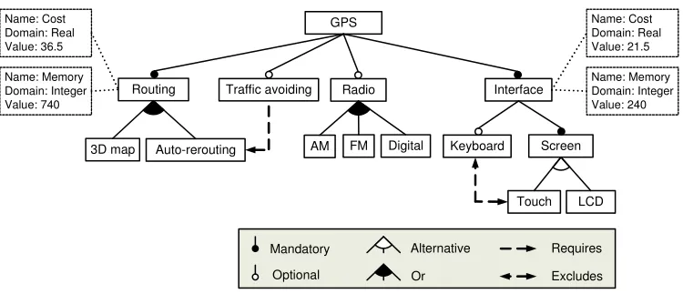
2006].Feature modelsare commonly used as a compact representation of all the prod-ucts in an SPL [Kang et al. 1990]. A feature model is visually represented as a tree-like structure in which nodes represent features, and connections illustrate the relation-ships between them. These relationrelation-ships constrain the way in which features can be combined to form valid configurations (products). For example, the feature model in Fig. 1 illustrates how features are used to specify and build software for Global Posi-tion System (GPS) devices. The software loaded into the GPS device is determined by the features that it supports. The root feature (‘GPS’) identifies the SPL. The following types of relationships constrain how features can be combined in a product.

—Mandatory. If a feature has a mandatory relationship with its parent feature, it must be included in all the products in which its parent feature appears. In Fig. 1, all GPS products must provide support forRouting.

—Optional. If a feature has an optional relationship with its parent feature, it can be optionally included in products that include its parent feature. For instance, Key-boardis defined as an optional feature of the userInterfaceof GPS products. —Alternative.A set of child features are defined as alternative if exactly one feature

should be selected when its parent feature is part of the product. In the example, GPS products must provide support for either aTouchscreen or anLCDscreen but not both in the same product.

—Or-Relation.Child features are said to have an or-relation with their parent when one or more of them can be included in the products in which its parent feature appears. In Fig. 1, software for GPS devices can provide support for3D mapviewing, Auto-reroutingor both of them in the same product.

In addition to the parental relationships between features, a feature model can also contain cross-tree constraints between features. These are typically of the form:

—Requires.If a feature A requires a feature B, the inclusion of A in a product implies the inclusion of B in this product. For example, GPS devices withTraffic avoiding require theAuto-reroutingfeature.

—Excludes. If a feature A excludes a feature B, both features cannot be part of the same product. In Fig. 1, GPS devices withTouch screen exclude the support for a Keyboard.

GPS

Routing Interface

Screen

LCD Touch Traffic avoiding

Auto-rerouting Keyboard

3D map

Mandatory

Optional

Alternative

Or

Requires

Excludes

Name: Cost Domain: Real Value: 21.5

Name: Memory Domain: Integer Value: 240 Name: Cost

Domain: Real Value: 36.5

Name: Memory Domain: Integer Value: 740

Radio

AM FM Digital

[image:6.612.120.495.483.650.2]

(7)

Feature models can be extended with extra-functional information by means of fea-ture attributes. An attribute usually consists of a name, a domain and a value. Fig. 1 depicts several feature attributes using the notation proposed by Benavides et al. [Be-navides et al. 2005]. As illustrated, attributes can be used to specify extra-functional information such as cost or RAM memory required to support the feature. Similar to other authors, in this paper we assume that the attribute values are fixed.

The automated analysis of feature models deals with the computer-aided extraction of information from feature models. Catalogues with up to 30 analysis operations on feature models have been published [Benavides et al. 2010]. Typical analysis opera-tions allow us to know whether a feature model is consistent (it represents at least one product), the number of products represented by a feature model, or whether a feature model contains any errors. In this paper, we address the so calledoptimisation analy-sis operation [Benavides et al. 2010]. This operation takes an attributed feature model and a set of objective functions as inputs and returns one or more products fulfilling the criteria established by the functions. For instances, we might search for a GPS program minimising cost and memory consumption. The analysis of a feature model is supported by a number of tools including theFaMaframework [Trinidad et al. 2008], FeatureIDE [Th ¨um et al. 2014] and SPLAR [Mendonca et al. 2009].

2.2. Evolutionary many-objective optimisation algorithms

Evolutionary algorithms (EAs) are a class of population-based metaheuristic optimi-sation algorithms that simulate the process of natural evolution. EAs are often well suited to many-objective problems (MOPs) because 1) they ideally do not make any assumption about the underlying fitness landscape and the considered objectives can be easily added, removed, or modified; 2) their population-based search can achieve an approximation of an MOP’s Pareto front4_{, with each individual representing a trade-off} amongst the objectives.

Despite being the most popular selection criterion in the EMO area, Pareto domi-nance encounters difficulties in its scalability to optimisation problems with more than three objectives (many-objective optimisation problems) [Wagner et al. 2007; Ishibuchi et al. 2008; Li et al. 2014b]. Due to the exponential decrease of the portion of the space that one point dominates, Pareto dominance is less able to differentiate points in the space. Recently, non-Pareto algorithms (algorithms that do not use Pareto dominance as the main selection criterion) have been shown to be promising in dealing with many-objective optimisation problems [Deb and Jain 2014; Bader and Zitzler 2011; Yang et al. 2013; Ishibuchi et al. 2015]. They typically provide higher selection pressure searching towards the Pareto front than Pareto-based algorithms.

In this paper, we consider six EMO algorithms. One is a classic Pareto-based algo-rithm, NSGA-II [Deb et al. 2002], and the rest are five non-Pareto-based algorithms, Indicator-Based Evolutionary Algorithm (IBEA) [Zitzler and K ¨unzli 2004], three ver-sions of the decomposition-based algorithm MOEA/D (MOEA/D-WS [Zhang and Li 2007], MOEA/D-TCH [Zhang and Li 2007], and MOEA/D-PBI [Zhang and Li 2007]) and SPEA2+SDE [Li et al. 2014a]. Of these, only NSGE-II and IBEA have previ-ously been applied to the problem of product selection. IBEA is an indicator-based algorithm that uses a given performance indicator to guide the search. MOEA/D-WS, MOEA/D-TCH, and MOEA/D-PBI are three versions of the decomposition-based algo-rithm MOEA/D, which uses three decomposition functions, weight sum, Tchebycheff, and penalty-based boundary intersection, respectively. SPEA2+SDE modifies the

orig-4

An individualxis said to Pareto dominate an individualyifxis as good asyin all objectives and better

(8)

inal SPEA2 by a shift-based density estimation, in order to enable the algorithm to be suitable for many-objective problems. These EMO algorithms are representative in the EMO area and, apart from NSGA-II, all have been found to be effective in dealing with many-objective optimisation problems with certain characteristics [Wagner et al. 2007; Hadka and Reed 2012; Li et al. 2013; Li et al. 2014].

3. THE PROPOSED SIP METHOD

In this section we describe the components of the SIP method. We start by describing two approaches to optimisation that can be used with any EMO algorithm: one con-sidering all objectives to be equal (the (n+1) approach used in previous work) and the new approach that considers the number of constraints violated and then the other objectives (the 1+n approach). We then describe the novel representation.

3.1. Optimisation approach used

Before applying an EMO algorithm to optimise the objectives in SPL product selection, an important issue is how to ‘view’ these objectives. A feature model contains a number of constraints that define the valid products. For example, in Figure 1 there is the constraint that a product cannot have both a Keyboard and a Touch screen interface. In order to direct the search towards valid products, one objective is the number of constraints violated (we wish to minimise this).

One overall approach to optimisation is to treat all objectives equally, as done in most previous work5_.

APPROACH 1. The (n+1) approach: all the objectives are viewed equally in the opti-misation process of EMO algorithms.

This deals with all the objectives simultaneously and attempts to obtain a set of good trade-offs among them. However, as previously observed [Henard et al. 2015], a software engineer will typically only be interested in products that satisfy all of the constraints. In such situations, the above (n+1) approach may not be suitable since it does not reflect the interest in valid products. This suggests that there is one main objective (whether the product is valid) and the others are less important. We therefore also implemented a new approach to optimisation in which the first objective (number of constraint violations) is viewed as being the main objective and then the remaining objectives as equal secondary objectives to be optimised.

APPROACH 2. The first objective (number of constraint violations) is viewed as the main objective to be considered first and then the remaining objectives as secondary objectives to be optimised equally. We call this the1+n approach.

Specifically, we used two simple rules to compare individuals in EMO algorithms: 1) prefer the individual with fewer constraint violations and 2) prefer the individual with better fitness (determined by the remaining objectives) when the number of violated constraints is equal.

In EMO algorithms, there are two operations in which individuals are com-pared, mating selection and environmental selection. Mating selection, which provides promising individuals for variation, is implemented by choosing the best individual from the mating pool (a set of candidate individuals). The proposed rules can be di-rectly applied to this selection process: the individual having the fewest constraint violations is chosen, and if there exist several such individuals then the one with the best fitness is chosen (in the usual way).

5_{An exception is the PULL method of Sayyad, in which the number of constraints that fail is given a higher}

(9)

Environmental selection, which determines the survival of individuals in the popu-lation, is implemented in different ways in EMO algorithms. If the population evolves in a steady-status way [Durillo et al. 2009] in an algorithm, environmental selection is implemented when only one new individual is produced. In this situation, the proposed rules can also be directly applied to the comparison between the new individual and some (or all) old ones in the population, as done in mating selection. On the other hand, if the population evolves in a generational way in an EMO algorithm, environmental selection is implemented when a set of new individuals is produced, where the size of the set is typically equal to the population sizeN. In this situation,N individuals will be chosen (to construct the next population) from a mixed set of the last popu-lation and the newly produced individuals on the basis of the proposed rules. Here, we group individuals of the mixed set into the next population according to their con-straint violations, i.e., individuals with the fewest concon-straint violations being chosen first, individuals with second fewest constraint violations second, and so on. This pro-cedure is continued until the population is full, or not full but cannot accommodate the next group of individuals with a particular value for the number of constraint vi-olations. The second case happens quite often since there could be many individuals with the same number of constraint violations. In this case, the selection strategy of the considered EMO algorithm is used to choose some of the individuals from the next group to fill the remaining slots of the population.

This property, of having one main goal, is not one normally found in many-objective optimisation. Typically, for a many-objective optimisation problem there is no hierar-chy among objectives and different decision makers may have different preferences for the objectives. Consequently, EMO algorithms typically search for a set of solutions representing the whole Pareto optimal front (i.e., a set of representative trade-offs among objectives), so that the decision maker can select one from these solutions ac-cording to his/her preference.

The constraint-handling method described above is similar to Deb et al.’s in NSGA-II [Deb et al. 2002], but with the following differences. NSGA-NSGA-II integrates constraint handling into the Pareto dominance relation and only considers the comparison be-tween two individuals; in contrast, the 1+n method is more general since it is designed to compare and select any number of individuals, thus being suitable for any EMO algorithm. In addition, in NSGA-II the fitness comparison is activated only when both individuals are valid (i.e., no constraint violations), while in the 1+n method the fitness comparison is made when the considered individuals have the same number of violated constraints. This is more suitable for the considered problem, since most individuals in the search process are invalid, with many having the same number of constraint violations.

3.2. A novel representation

The natural representation, which was used previously [Sayyad et al. 2013d], is to represent a product as a binary string where for a featureFithere is a corresponding

gene, with value 1 _{if the product contains}_Fi and otherwise0. This is a direct

repre-sentation of the set of features in a product. In initial experiments with the E-shop and WebPortal case studies6_{(Section 5) we found that many of the products returned} were invalid and this is consistent with the observations of Sayyad et al. [Sayyad et al. 2013d].

We conjectured that performance was adversely affected by the following patterns.

6_{We used experiments with these two case studies to explore the nature of the problem. Once we settled on}

(10)

(1) The failure to include core features (features that are contained in all valid prod-ucts). The initial work by Sayyad et al. [Sayyad et al. 2013d] did not take these into account but their enhanced version did [Sayyad et al. 2013c] as did Henard et al. [Henard et al. 2015].

(2) The inclusion of one or more children of a feature F even thoughF is not in the product.

In the first case the problem is that any set of features that fails to contain a core featureFmust be invalid. To tackle this issue we simply removed all core features from the representation; such features would be added back into the candidate solutions at the end of the search. Core features were found using the SPLAR tool [Mendonca et al. 2009]. This change to the representation immediately avoids the inclusion of some invalid products and was used by Sayyad et al. in their second paper on this topic [Sayyad et al. 2013c] and later by Henard et al. [Henard et al. 2015]. It would also have been possible to remove any dead features that were present (features that appear in no valid products). However, sensible feature models do not contain dead features and tools such as FaMa [Benavides et al. 2007] and SPLAR [Mendonca et al. 2009] can be used to detect dead features.

For the second case, the problem is that if a featureF′ _{is in a product and}_F′ _has

parentF that is not in the product then the product cannot be valid. This pattern is entirely syntactic and it is straightforward to identify cases where it occurs. Further, in such a case the inclusion ofF′_{implies the inclusion of}_F_{. This might suggest that we}

only need include leaf features in our representation. However, this is not quite right since it excludes the case where a featureF is in a product but none of its children are in the product (they are optional); such a representation could therefore exclude some valid products. We therefore excluded a feature F if the following property holds: F has one or more children and is involved in a relationship that is either aMandatory, Alternative, orOrrelationship (Optionalrelationships have no effect). If this property holds thenF is included in a valid product if and only if one or more of its children are in the product. Thus, there is no need to includeFin the representation and we addF to a set of features returned by the search if and only if one or more of its children are in the set. A parent featureF added using this step may, itself, be a child of a feature that is not in the set and so this second rule is applied repeatedly until no more features can be added. The number of iterations of this process is at most the depth of the tree representing the feature model and this process takes time that is linear in the size of the feature model. A featureFis kept if there is an Optional relationship with all of its children since it is possible for a valid product to includeF but no children ofF. This is one way in which invalid products can result: we might have a product that does not includeF but does include one or more of its children. Invalid products can also result from cross-tree constraints.

(11)

(1) The representation is smaller, as well as the search space, as a consequence. (2) It is not possible to represent products that contain one or more of FM, AM and

Digital but do not include the feature Radio. This is useful because all such prod-ucts are invalid.

In principle it might be possible to further adapt the representation by taking into account cross-tree constraints. We might also have adapted the representation so that only one child in an Alternative relationship could be included. We see the further development of the representation, to ensure that additional constraints must be sat-isfied, as a topic for future work.

The overall (novel) encoding is therefore to use a binary string, where there is a valuevifor featureFiif and only ifFiis not core and alsoFidoes not have one or more

children that are in a Mandatory, Or, or Alternative relation. If the search returns a set P′ _{of features then we generate the corresponding candidate product by applying}

the following steps.

(1) Add toP′ _{all core features.}

(2) Add toP′ _{any feature}_F _{not in}_P′ _{such that}_P′ _{contains one or more children of}_F

and apply this step repeatedly until no more features can be added.

In the experiments we compared the following representations.

(1) That initially used by Sayyad et al. [Sayyad et al. 2013d]. We called this thedirect encodingsince each feature has a corresponding bit in the representation.

(2) That used in the second paper of Sayyad et al. [Sayyad et al. 2013c] and also by Henard et al. [Henard et al. 2015]. We called this thecore encodingsince we do not represent the core features.

(3) A representation in which we retain core features but do not include a feature if the following holds: the feature is included in a valid product if and only if one or more of its children are in the product. We called this thehierarchical encoding. (4) The novel representation outlined in this section, which is the combined

applica-tion of (2) and (3). We called this thenovel encoding.

We included the third representation in order to be able to separately assess the two enhancements in the novel encoding. However, this representation was only used in the initial experiments: the main focus of the experiments was to compare our novel encoding with the previously proposed direct and core encodings.

The representations, for the GPS example, are given in Table I.

To conclude, the proposed SIP method is to use: the novel encoding; the 1+n ap-proach; and an EMO algorithm.

4. EXPERIMENTAL DESIGN

(12)

per-Table I. Features included in each encoding on the GPS SPL

Feature Encoding

Direct Core Hierarchical Novel

GPS X X

Routing X X

3D map X X X X

Auto-rerouting X X X X

Traffic avoiding X X X X

Radio X X

FM X X X X

AM X X X X

Digital X X X X

Interface X X

Keyboard X X X X

Screen X X

Touch X X X X

LCD X X X X

formed 30 times to reduce the impact of the stochastic nature of the algorithms. We now describe the research questions.

First, there is the question of whether the encoding used affects the performance of the search and, within this, whether the novel encoding is more effective than the previously used direct and core encodings.

RESEARCHQUESTION 1. How does the encoding affect the performance of the search techniques?

Our additional enhancement was to consider the first objective as the main objective, with the aim being to direct search towards valid products.

RESEARCHQUESTION 2. Does the use of the 1+n approach make it easier for the search techniques to find valid products?

Previous work has found that Pareto based techniques are relatively ineffective when using the direct and core encodings and so most of the search techniques used were not based on Pareto dominance. We were interested in whether there were differ-ences in performance between the search techniques.

RESEARCHQUESTION 3. Are particular EMO algorithms more effective than oth-ers?

Previous studies have used feature models with randomly generated attributes and this leads to a particular threat to validity, which is that these results might not trans-fer to feature models with realistic attributes.

RESEARCHQUESTION 4. Does the relative performance differ when realistic at-tribute values are used?

RESEARCHQUESTION 5. Is the relative performance similar when using a larger randomly generated feature model?

While it is important that the search returns valid products, ideally we would like many valid products to be returned.

[image:12.612.189.426.109.263.2]

(13)

Finally, we also care about execution time: if one approach is much quicker than the others then this approach can be allowed to run for more generations.

RESEARCHQUESTION 7. How does the execution time differ between approaches?

4.1. Experimental Subjects

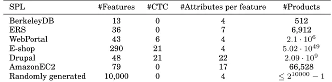
[image:13.612.141.472.364.446.2]

Table II depicts the attributed feature models used in the evaluation. For each model, the number of features, Cross-Tree Constraints (CTCs), feature attributes and prod-ucts are presented. The number of attributes gives the number of attributes that each feature has and so the total number of actual values used is the product of the num-ber of features and numnum-ber of attributes. We give an upper bound on the numnum-ber of products for the larger randomly generated model since it is not feasible to determine the number of products for such a large model. These models cover a range of sizes in terms of features and attributes. The models BerkeleyDB, ERS, WebPortal and EShop have been used in related works on optimal SPL product selection [Guo et al. 2014; Olaechea et al. 2014; Sayyad et al. 2013b; Sayyad et al. 2013a; Sayyad et al. 2013d]. We used Olaechea et al.’s [Olaechea et al. 2014] version of these models to obtain com-parable results. The larger examples used by Sayyard et al. and Henard et al. were written in the DIMACS notation, that provides input to SAT solvers; we did not use these since our method takes as input a feature model written in the SXFM format for feature models. However, we used two recently published feature models, AmazonEC2 and Drupal, with realistic attribute values derived from mining real systems.

Table II. Subject models

SPL #Features #CTC #Attributes per feature #Products

BerkeleyDB 13 0 4 512

ERS 36 0 7 6,912

WebPortal 43 6 4 2.1_·106

E-shop 290 21 4 5.02_·1049

Drupal 48 21 22 2.09_·109

AmazonEC2 79 0 17 66,528

Randomly generated 10,000 0 4 ≤210000

−1

BerkeleyDB [Siegmund et al. 2012] provides a high-level representation of variabil-ity in a database and ERS [Esfahani et al. 2013] represents variabilvariabil-ity in an Emer-gency Response System. Web Portal [Mendonca et al. 2008] and EShop [Lau 2006] rep-resent a product line of web portals and e-commerce applications respectively. Sayaad et al. [Sayyad et al. 2013b; Sayyad et al. 2013a; Sayyad et al. 2013d] and Olaechea et al [Guo et al. 2014; Olaechea et al. 2014] extended these models with three features attributes with randomly generated values: cost, defects and prior usage count. We followed the same approach in this work.

Drupal [S ´anchez et al. 2015] represents the variability in the open source Web con-tent management framework Drupal. The model is provided with values of 22 non-functional attributes extracted from the Drupal GIT repository and the Drupal issue tracking system including, among others, size, changes, defects, cyclomatic complexity, test cases, developers and reported installations. To the best of our knowledge, this is the largest attributed feature model with non-synthetically generated attributes used for the problem of optimal SPL product selection.

(14)

usage and defaultStorage. Attributes in AmazonEC2 do not have a fixed value. In-stead, the value of each attribute is derived from the selected features using thou-sands of constraints of the form “M2 xlarge IMPLIES (Instance.cores==2 AND

Instance.ram==17.1)”. For each of these, we assigned a random value to each attribute

within its domain.

Experiments were also performed on a larger, randomly generated, feature model with 10,000 features. This was generated using the SPLAR tool [Mendonca et al. 2009] and with the following parameters: 25% mandatory features; 25% optional features; 25% alternative features; minimum branching factor of 5; maximum branching factor of 10; maximum size for feature groups of 5; and only consistent models. These values have been found to be typical values for feature models [Th ¨um et al. 2009].

To summarise, we used four models that have previously been used so that our re-sults can be compared with other studies. We used two additional real feature models (Drupal, Amazon) since we had access to realistic attribute values (either real val-ues or ranges). Finally, we added a randomly generated model with 10,000 features in order to evaluate the approaches on a large model.

4.2. The optimisation problems

In the initial experiments we used the same five objectives as Sayyad et al. [Sayyad et al. 2013d] and Henard et al. [Henard et al. 2015].

(1) Correctness: the number of constraints that were not satisfied. This value should be minimised.

(2) Richness of features: how many features were included. This value should be max-imised, preferring products with many features.

(3) Features that were used before. For each feature this is a boolean and the number for which this is true should be maximised (previously used features are less likely to be faulty and those used before are likely to be more popular).

(4) Known defects: the number of known defects in features used should be minimised. There is a constraint on this value: it has to be zero if the feature was not used before.

(5) Cost: the sum of the costs of the features included. This value should be minimised.

We used the above objectives in order to be consistent with previous work. However, as previously discussed, we included additional experiments in which we used realistic values for attributes. Since we did not have information on all of the above attributes, we instead used eight objectives for which we had realistic values. For Drupal we used the following objectives.

(2) Richness of features: how many features were included. This value should be max-imised.

(3) Number of lines of code. This should be minimised. (4) Cyclomatic complexity. This should be minimised. (5) Test Assertions. This should be maximised.

(6) Number of installations that contain the feature. This should be maximised. (7) Number of developers. This should be minimised.

(8) Number of changes. This should be minimised.

We want to minimise the last two (number of developers and number of changes) since there is evidence that these correlate with how error prone a system is [Mat-sumoto et al. 2010; Yoo and Harman 2012].

(15)

(2) Richness of features: how many features were included. This value should be max-imised, preferring products with many features.

(3) EC2.costMonth: (random value from 0 to 20000). This value should be minimised. (4) Instance.cores: (random value from 1 to 32). This value should be maximised. (5) Instance.ecu: (random value from 0 to 108). This value should be maximised. (6) Instance.ram: (random value from 0 to 250). This value should be maximised. (7) Instance.costHour: (random value from 0 to 18). This value should be minimised. (8) Instance.ssdBacked: (Boolean). This value should be maximised.

Finally, we included experiments with the larger randomly generated feature model (with 10,000 features). For this we used the original five objectives, again to be consis-tent with earlier work.

4.3. Implementation details

All the EMO algorithms were executed 30 times for each experiment to reduce the impact of their stochastic nature. The termination criterion used in all the algorithms was a predefined number of evaluations, which was set to 50,000 unless otherwise mentioned. The size of the population for all the algorithms except MOEA/D was set to 100. The population size in MOEA/D, which is the same as the number of weight vectors, cannot be arbitrarily specified. Following the practice in [Yang et al. 2013], we used the closest integer to 100 amongst the possible values as the population size of the three MOEA/D algorithms (126 and 120 for the 5- and 8-objective problems, respectively).

Some of the algorithms require several parameters to be set. As suggested in their original papers [Zhang and Li 2007; Zitzler and K ¨unzli 2004], the neighbourhood size was set to 10% of the population size in the three MOEA/D algorithms, the penalty parameterθto 5 in MOEA/D-PBI, and the scaling factorκto 0.05 in IBEA.

Two widely-used crossover and mutation operators in combinatorial optimisation problems, uniform crossover and bit-flip mutation, were used. A crossover probability pc= 1.0and a mutation probabilitypm= 1/n(wherendenotes the number of decision

variables) were set according to [Deb 2001]. As a result of using recommended values from the literature, we did not require a tuning phase.

All the experiments were performed on a notebook PC with Intel(R) Core(TM)i5-3230M Quad [email protected] GHz with 4GB of RAM. We obtained implementations of the EMO algorithms from standard toolkits7_.

4.4. Performance metrics

We used three performance metrics to study the results of the experiments. Hyper-volume (HV) [Zitzler and Thiele 1999] is a very popular metric in the EMO area due to its good theoretical and practical properties, such as being compliant with Pareto dominance (if one population Pareto dominates another then it has a higher HV) and not requiring the problem’s Pareto front to be known. HV calculates the volume of the objective space between the obtained solution set and a reference point. A large value is preferable and reflects good performance of the solution set in terms of con-vergence, extensity and uniformity. Figure 2 gives an illustration of the HV metric for four solution sets with different performance. As shown, the solution set that has good

7

(16)

(a) (b) (c) (d)

Fig. 2. HV result (shaded area) for four sets of solutions with respect to a bi-objective minimisation problem scenario. (a) Solution set with good convergence, extensity and uniformity. (b) Solution set with good exten-sity and uniformity, poor convergence. (c) Solution set with good convergence and uniformity, poor extenexten-sity. (d) Solution set with good convergence and extensity, poor uniformity.

convergence, extensity and uniformity (Figure 2(a)) leads to a larger shaded area (HV value) than the other three solution sets which have poor convergence, extensity or uniformity, respectively (Figure 2(b)–(d)).

In the calculation of HV, two crucial issues are the scaling of the search space [Friedrich et al. 2009] and the choice of the reference point [Auger et al. 2009]. Since the objectives in the considered optimisation problems take different ranges of values, we normalised the objective value of the obtained solutions according to the problem’s range in the objective space. Also, the reference point was set to the Nadir point of the problem’s range (the point constructed with the worst value on each objective). In addition, note that the exact calculation of the HV metric is often infeasible for a solu-tion set with seven or more objectives and so for the problems with eight objectives we estimated the HV result of a solution set by the Monte Carlo sampling method used by Bader and Zitzler [Bader and Zitzler 2011]. Here, 10,000,000 sampling points were used to ensure accuracy [Bader and Zitzler 2011].

Since the software engineer is only interested in valid products, we also introduced two metrics to evaluate the ability of each algorithm to return valid products. These metrics are: 1) the number of executions where there was at least one valid individual in the final population, denoted VN; and 2) the rate of valid individuals in the final population, denoted VR.

Finally, it is necessary to mention that in computing HV, we only used the valid solutions in the population (as invalid solutions could be meaningless for the decision maker). As a result, we computed HV using only the valid individuals in the final population and so used all objectives except the first one (the number of constraints violated). In addition, the results of HV and VR given in the tables were averaged over the executions where at least one valid individual was returned. In cases where valid solutions were not produced in any of the 30 executions (V N = 0), we reported0 for HV and VR.

Since invalid products have no value, the most important metric is the value of VN. A high value for VR means that the software engineer has many valid products from which to choose and, a high value for HV means that these have good performance in terms of convergence and diversity.

5. RESULTS

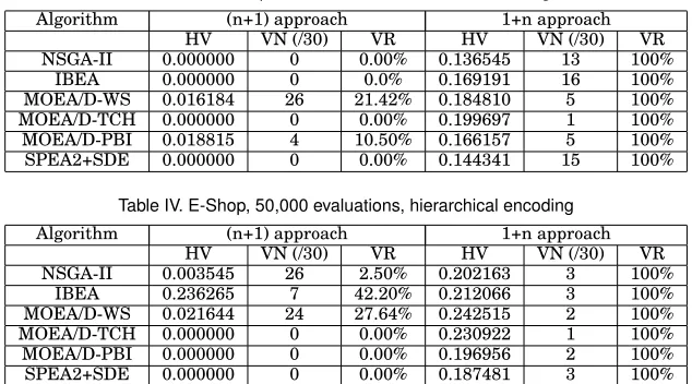
[image:16.612.110.505.94.185.2]

(17)

[image:17.612.149.466.101.277.2]

Table III. E-Shop, 50,000 evaluations, direct encoding

Algorithm (n+1) approach 1+n approach

HV VN (/30) VR HV VN (/30) VR

NSGA-II 0.000000 0 0.00% 0.136545 13 100%

IBEA 0.000000 0 0.0% 0.169191 16 100%

MOEA/D-WS 0.016184 26 21.42% 0.184810 5 100%

MOEA/D-TCH 0.000000 0 0.00% 0.199697 1 100%

MOEA/D-PBI 0.018815 4 10.50% 0.166157 5 100%

SPEA2+SDE 0.000000 0 0.00% 0.144341 15 100%

Table IV. E-Shop, 50,000 evaluations, hierarchical encoding

NSGA-II 0.003545 26 2.50% 0.202163 3 100%

IBEA 0.236265 7 42.20% 0.212066 3 100%

MOEA/D-WS 0.021644 24 27.64% 0.242515 2 100%

MOEA/D-TCH 0.000000 0 0.00% 0.230922 1 100%

MOEA/D-PBI 0.000000 0 0.00% 0.196956 2 100%

SPEA2+SDE 0.000000 0 0.00% 0.187481 3 100%

(Hypervolume), VN (number of executions where there was at least one valid individ-ual in the final population) and VR (the rate of valid individindivid-uals in the population on average for the executions where there was at least one valid individual in the final population). The software engineer is only interested in valid products and so we say than an approach is effective if it often returns valid products.

5.1. The E-shop and WebPortal case studies

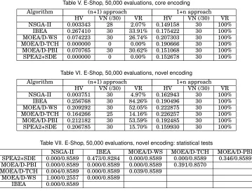
Initial experiments were carried out using E-shop and WebPortal and with four encod-ings: the direct encoding; the core encoding (where core features are removed); the hi-erarchical encoding (where some parents are removed); and the novel encoding. The re-sults for E-shop, with 50,000 evaluations, can be found in Tables III-VI. First consider the (n+1) approach. This was relatively ineffective with the direct encoding, with most techniques failing to return valid products. The main exception to this is MOEA/D-WS, which returned valid products in 26 of the 30 runs. The performance with the hierar-chical encoding was not much better, though interestingly NSGA-II also produced valid products on most runs. For both of these, the performance of IBEA was relatively poor. The performance with the core encoding was superior, with several of the search tech-niques returning valid products on most or all executions. Further improvements can be found with the novel encoding: all but one search technique returned valid products on all executions. For this case, IBEA gave the largest number of valid solutions (a VR of 84.26%) and the highest HV. The performance of the 1+n approach was particularly impressive. For both the core and novel encoding, all solutions returned were valid (a VN of 30 and VR of 100%). For both of these encodings, WS and MOEA/D-TCH had the highest HV values. Note that the 1+n approach always returned a VR value of 100%, even for cases where the (n+1) approach had a low VN value. One ex-planation is that, once the search has found a valid product it is able to find additional valid products from this (similar to the use of a seed by Sayyad et al. [Sayyad et al. 2013c]) and the search prioritises these above any invalid products.

(18)

[image:18.612.126.485.93.369.2]

Table V. E-Shop, 50,000 evaluations, core encoding

NSGA-II 0.003343 28 2.07% 0.149158 30 100%

IBEA 0.267410 30 33.91% 0.175422 30 100%

MOEA/D-WS 0.074223 30 26.74% 0.207303 30 100%

MOEA/D-TCH 0.000000 0 0.00% 0.190666 30 100%

MOEA/D-PBI 0.070765 30 30.62% 0.151068 30 100%

SPEA2+SDE 0.000000 0 0.00% 0.152678 30 100%

Table VI. E-Shop, 50,000 evaluations, novel encoding

NSGA-II 0.003751 30 4.97% 0.162943 30 100%

IBEA 0.256768 30 84.26% 0.190496 30 100%

MOEA/D-WS 0.209292 30 52.05% 0.222875 30 100% MOEA/D-TCH 0.164266 25 14.16% 0.226257 30 100% MOEA/D-PBI 0.212182 30 53.59% 0.192485 30 100% SPEA2+SDE 0.206785 30 15.70% 0.159930 30 100%

Table VII. E-Shop, 50,000 evaluations, novel encoding: statistical tests

NSGA-II IBEA MOEA/D-WS MOEA/D-TCH MOEA/D-PBI SPEA2+SDE 0.000/0.8589 0.473/0.8284 0.000/0.8589 0.000/0.8589 0.346/0.8589 MOEA/D-PBI 0.000/0.8589 0.000/0.8589 0.000/0.8589 0.391/0.8570

MOEA/D-TCH 0.004/0.8589 0.000/0.8589 0.039/0.8589 MOEA/D-WS 1.000/0.2557 0.000/0.8589

IBEA 0.000/0.8589

SPSS) for pairwise comparisons of the six algorithms. In all of the experiments the final p-value between two algorithms was obtained after the Bonferroni adjustment was made (this step will not be described again). We also used the Mann-Whitney U test to calculate the effect size (ES) of pair-wise algorithms. First the standardised test statistic Z was obtained by the Mann-Whitney U test (implemented by SPSS). Then the ES was calculated usingES = Z

√_N whereN is the total number of samples. The

results for E-shop are given in Table VII, where a cell having contentsx/ydenotes the p-value beingxand the effect size beingy.

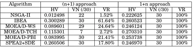
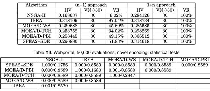
The results for WebPortal (Tables VIII-XI) and 50,000 evaluations are generally bet-ter than those for E-shop. All settings led to valid products being returned on at least 7 occasions and the 1+n approach returned no invalid products. In contrast to E-shop, IBEA returned the highest HV values. Again, we used statistical tests to compare the HV values returned by the algorithms when using the novel encoding and 1+n ap-proach. The results of the post-hoc Kruskal-Wallis test and the effect size are shown in Table XII.

We also carried out experiments with E-shop and 500,000 evaluations to see whether this increase in number of evaluations affects performance. The results of these exper-iments can be found in the Appendix (Tables XXV-XXVIII). The patterns are similar to the results with 50,000 evaluations but it is worth noting that NSGA-II is effective with even the direct encoding. As before, only valid products were returned with the core and novel encoding with the 1+n approach and MOEA/D-WS and MOEA/D-TCH had the highest HV values for these cases.

(19)

[image:19.612.143.469.90.384.2]

Table VIII. WebPortal, 50,000 evaluations, direct encoding

NSGA-II 0.012498 22 1.52% 0.222625 30 100%

IBEA 0.300289 30 61.64% 0.260523 30 100%

MOEA/D-WS 0.089601 29 24.64% 0.246124 30 100%

MOEA/D-TCH 0.115301 7 2.72% 0.270310 30 100%

[image:19.612.151.466.103.181.2]

MOEA/D-PBI 0.083995 30 21.41% 0.253738 30 100% SPEA2+SDE 0.260506 30 17.80% 0.246970 30 100%

Table IX. WebPortal, 50,000 evaluations, hierarchical encoding

NSGA-II 0.119382 30 2.60% 0.281518 30 100%

IBEA 0.314488 30 88.67% 0.315128 30 100%

Table X. WebPortal, 50,000 evaluations, core encoding

NSGA-II 0.059950 30 1.70% 0.275413 30 100%

IBEA 0.308381 30 78.99% 0.307052 30 100%

HV values for 500,000 were higher than the HV values for 50,000. It may well be that we would obtain even better results if the number of evaluations was increased further. We followed the same statistical procedure as before. The results of the post-hoc Kruskal-Wallis test and the effect size are shown in the Appendix (Table XXIX).

5.2. The remaining case studies using published feature models

We carried out experiments with Amazon, Berkeley, Drupal, and ERS in order to check whether the results for E-Shop and WebPortal extended to other models (the results of the experiments using Amazon and Drupal with realistic attribute values are de-scribed in the next section). As before, we used the two approaches: 1+n; and (n+1). Previously, we carried out experiments with four encodings, using the hierarchical encoding to check that this was not as effective as the novel encoding (i.e. that the enhancements in the core encoding still have value when also using the hierarchical encoding). Having confirmed this, there was no need to carry out additional experi-ments with the hierarchical encoding. Thus, for the remaining case studies we used the two previously published encodings (direct and core) and the encoding proposed in this paper (the novel encoding).

(20)

bet-Table XI. WebPortal, 50,000 evaluations, novel encoding

NSGA-II 0.168637 30 6.02% 0.284126 30 100%

IBEA 0.318109 30 97.04% 0.318734 30 100%

Table XII. Webportal, 50,000 evaluations, novel encoding: statistical tests

IBEA 0.001/0.8570

ter at finding valid solutions but sometimes returned a less diverse population. Finally, observe that most techniques performed poorly in the experiments using the direct and core encodings and the (n+1) approach; IBEA is the exception to this since it always found at least one valid product. We followed the same statistical procedure as before. The results of the post-hoc Kruskal-Wallis test and the effect size are shown in the Appendix (Table XXXIII).

Consider now the results with the Berkeley feature model (Appendix, Tables XXXIV, XXXV and XXXVI). This appears to be a simpler problem, possibly due to having a rel-atively small number of products and attributes, with all combinations of encoding and approach to optimisation always returned some valid products. However, only the 1+n approach (all three encodings) always returned only valid products (V R= 100%_{). For}

the 1+n approach there appears to be relatively little difference in the different encod-ings. In contrast, if we use the (n+1) approach then the novel encoding outperforms the core encoding and this, in turn, outperforms the direct encoding. Table XXXVII in the Appendix gives the results of the post-hoc Kruskal-Wallis test and effect size for the EMO algorithms when using the novel encoding and 1+n approach.

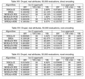
Similar to Berkeley, the results with Drupal (Appendix, Tables XXXVIII, XXXIX and XL) suggest that this is a simpler search problem. With the 1+n approach, all combi-nations of encoding and algorithm always returned a population of valid solutions. For the (n+1) approach we find a more varied performance. We again found that the novel encoding outperformed the core encoding and this outperformed the direct encoding. We find that MOEA/D-TCH only returned valid solutions in one of the 30 executions. With the novel encoding and 1+n approach IBEA had the highest HV value. Table XLI in the Appendix gives the results of the post-hoc Kruskal-Wallis test and effect sizes for the EMO algorithms when using the novel encoding and 1+n approach.

[image:20.612.119.488.101.262.2]

(21)

[image:21.612.143.471.91.395.2]

Table XIII. Drupal, real attributes, 50,000 evaluations, direct encoding

NSGA-II 0.000002 30 2.60% 0.074917 30 100%

IBEA 0.122192 30 41.13% 0.123803 30 100%

MOEA/D-WS 0.081417 30 19.12% 0.116287 30 100%

MOEA/D-TCH 0.037675 7 1.62% 0.117087 30 100%

MOEA/D-PBI 0.085339 30 19.37% 0.013610 29 100% SPEA2+SDE 0.100164 30 9.57% 0.131757 30 100%

Table XIV. Drupal, real attributes, 50,000 evaluations, core encoding

NSGA-II 0.000565 30 3.82% 0.074595 30 100%

IBEA 0.129126 30 62.47% 0.122216 30 100%

[image:21.612.149.467.200.288.2]

Table XV. Drupal, real attributes, 50,000 evaluations, novel encoding

NSGA-II 0.015450 30 6.92% 0.076093 30 100%

IBEA 0.128167 30 80.13% 0.129285 30 100%

5.3. Experiments with realistic attributes

As previously explained, we performed experiments with the Amazon and Drupal case studies using eight attributes for which we either had real attribute values or we had ranges from which we could generate values. The results for Drupal can be found in Tables XIII-XV in which the 1+n approach always returned only valid products. For all three encodings, when we used the 1+n approach we found that SPEA2+SDE returned the highest HV value. As before, the novel encoding produced slightly better results than the core encoding (slightly higher HV values). Table XVI gives the results of the post-hoc Kruskal-Wallis test and the effect size values for the EMO algorithms when using the novel encoding and 1+n approach.

[image:21.612.148.466.302.385.2]

(22)

[image:22.612.128.476.85.368.2]

Table XVI. Drupal, real attributes, 50,000 evaluations, novel encoding: statistical tests

[image:22.612.120.494.103.165.2]

IBEA 0.000/0.8589

Table XVII. Amazon, realistic attributes, 50,000 evaluations, direct encoding

NSGA-II 0.000000 0 0% 0.001023 30 100%

IBEA 0.000000 0 0% 0.001328 1 100%

MOEA/D-WS 0.000375 1 1.67% 0.000926 22 100%

MOEA/D-TCH 0.000000 0 0% 0.000000 0 0%

MOEA/D-PBI 0.000000 0 0% 0.000000 0 0%

SPEA2+SDE 0.000000 0 0% 0.000935 27 100%

Table XVIII. Amazon, realistic attributes, 50,000 evaluations, core encoding

NSGA-II 0.000000 0 0% 0.000976 30 100%

IBEA 0.000000 0 0% 0.000000 0 0%

MOEA/D-WS 0.000126 1 1.72% 0.000954 23 100%

MOEA/D-TCH 0.000000 0 0% 0.000000 0 0%

MOEA/D-PBI 0.000000 0 0% 0.000000 0 0%

SPEA2+SDE 0.000000 0 0% 0.001125 29 100%

5.4. Experiments with a larger feature model

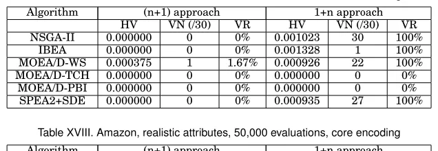
This subsection contains the result of the experiments performed with a larger ran-domly generated feature model. As previously stated, for this we used five objectives and applied three different encodings (direct, core and novel) and the two different approaches ((n+1) vs. 1+n). Interestingly, none of the experiments with the direct and core encodings returned valid products (and so we do not include tables for these exper-iments). The results of the experiments with the novel encoding are given in Table XXI. The results reinforce some of the previous observations but there are larger differences for this model. The key observation is that the choice of representation and approach appears to be crucial: we only obtained valid products when using the novel encoding and the 1+n approach. Amongst the techniques that return valid solutions (for the novel encoding and 1+n approach), SPEA2+SDE appears to have performed best since it returned valid products on almost all executions. However, it had a relatively low HV score suggesting that it returned less diverse populations. Both MOEA/D-PBI and MOEA/D-WS returned much higher HV values, indicating a more diverse population, but also found valid products less frequently. Table XXII gives the results of the post-hoc Kruskal-Wallis test and the effect sizes for the EMO algorithms when using the novel encoding and 1+n approach.

[image:22.612.147.465.183.293.2]

(23)

[image:23.612.123.484.84.364.2]

Table XIX. Amazon, realistic attributes, 50,000 evaluations, novel encoding

NSGA-II 0.000306 30 1.78% 0.001844 30 100%

IBEA 0.000000 0 0% 0.001897 17 100%

MOEA/D-WS 0.001158 30 19.68% 0.001877 30 100%

MOEA/D-TCH 0.000000 0 0% 0.001688 30 100%

MOEA/D-PBI 0.001017 25 10.97% 0.000000 0 0%

[image:23.612.147.467.102.183.2]

SPEA2+SDE 0.000000 0 0% 0.002001 30 100%

Table XX. Amazon, realistic attributes, 50,000 evaluations, novel encoding: statistical tests NSGA-II IBEA MOEA/D-WS MOEA/D-TCH MOEA/D-PBI SPEA2+SDE 0.005/0.5536 0.001/0.6718 1.000/0.3513 0.000/0.7693 0.000/0.9182 MOEA/D-PBI 0.000/0.9182 0.000/0.8473 0.000/0.9182 0.000/0.9182

IBEA 1.000/0.1773

Table XXI. Random model, 50,000 evaluations, novel encoding Algorithm (n+1) approach 1+n approach

NSGA-II 0 0 0% 0.014588 24 100%

IBEA 0 0 0% 0.020762 25 100%

MOEA/D-WS 0 0 0% 0.042142 15 100%

MOEA/D-TCH 0 0 0% 0.025037 19 100%

MOEA/D-PBI 0 0 0% 0.042513 18 100%

SPEA2+SDE 0 0 0% 0.018173 28 100%

is the slowest EMO algorithm, IBEA is the second slowest, and the other four have similar performance.

6. DISCUSSION

We now explore the results and what they tell us about the research questions.

6.1. Research Question 1: The importance of the encoding

It is clear that the encoding does matter: the novel encoding consistently outperformed the direct encoding and also both the core and hierarchical encodings (where these were evaluated). This was both for the case where all objectives are considered together and the 1+n approach. Interestingly, the novel encoding significantly outperformed the core encoding in the experiments with Amazon with realistic attributes. The strongest result was with the larger randomly generated model, where the SIP method (using the novel encoding and the 1+n approach) was the only one that returned valid prod-ucts. The results indicate that the encoding does affect performance, with the novel encoding proving to be most effective.

6.2. Research Question 2: The value of using the 1+n approach

(24)

[image:24.612.115.495.106.167.2] [image:24.612.135.464.106.360.2]

Table XXII. Random model, 50,000 evaluations, novel encoding: statistical tests

IBEA 0.000/0.7746

Table XXIII. Time taken in seconds, randomly generated model

Encoding EMO algorithm (n+1) 1+n

Direct encoding

NSGA-II 132.326000 131.444000 IBEA 165.169000 158.104000 MOEA/D-WS 148.954660 142.332000 MOEA/D-TCH 159.605793 145.403000 MOEA/D-PBI 164.638539 150.022000 SPEA2+SDE 596.126000 145.257000

Core encoding

NSGA-II 105.831000 103.188000 IBEA 147.404000 132.454000 MOEA/D-WS 136.588161 115.169000 MOEA/D-TCH 145.6549118 108.499000 MOEA/D-PBI 141.3576826 112.164000 SPEA2+SDE 428.576000 168.624000

Novel encoding

NSGA-II 101.760000 98.758000 IBEA 154.399000 131.465000 MOEA/D-WS 135.978589 104.442000 MOEA/D-TCH 132.905541 99.700000

MOEA/D-PBI 131.915617 102.999000 SPEA2+SDE 247.786000 223.777000

used the novel encoding and 1+n approach. The results suggest that the 1+n approach was more effective than the (n+1) approach.

6.3. Research Question 3: The relative performance of the EMO algorithms

An interesting initial observation is that there is no ‘clear winner’, in contrast to pre-vious work that found IBEA to be superior to other techniques. One possible expla-nation for this is our use of a range of EMO algorithms that are not based on Pareto dominance. However, there is a second explanation which is that the best results were obtained with the novel encoding and the 1+n approach: this is not a representation or approach previously used.

(25)

[image:25.612.125.490.100.208.2]

Table XXIV. Best performing EMO algorithm, novel encoding and 1+n Subject model Best performing MOEA Superior to all except E-Shop 50,000 MOEA/D-TCH MOEA/D-WS, MOEA/D-PBI

E-Shop 500,000 MOEA/D-WS MOEA/D-TCH

WebPortal IBEA MOEA/D-PBI

Amazon SPEA2+SDE NSGA-II, IBEA, MOEA/D-WS, MOEA/D-TCH

Berkeley SPEA2+SDE IBEA

Drupal IBEA MOEA/D-PBI

ERS NSGA-II SPEA2+SDE, MOEA/D-TCH, MOEA/D-WS

Drupal, real SPEA2+SDE IBEA

Amazon, realistic SPEA2+SDE MOEA/D-WS

Larger model SPEA2+SDE NSGA-II, IBEA

The main point is that there is no clear ‘best’ EMO algorithm. In fact, in contrast to earlier work, there is one subject for which NSGA-II outperforms all others. While in many cases SPEA2+SDE provided the best performance, experiments found this to be the slowest technique and any differences in performance may well be negated by this factor.

Note that one would expect the best performing algorithm to depend on the nature of the given product selection optimisation problem. For example, SPEA2+SDE has been found to perform well with problems in which convergence is difficult, such as those with a large number of objectives. Thus, it might be a good choice if the software engineer has a particularly large feature model or there is a large number of objectives. The three MOEA/D algorithms are suitable for problems in which it is hard to find a set of widely-distributed valid products. IBEA is a good choice for the decision maker who is more interested in the boundary solutions (i.e., the products having extreme value of one or several objectives) of the problem.

6.4. Research Question 4: The effect of using realistic attribute values

The results for this were quite similar, in that the novel encoding and the 1+n ap-proach both led to improvements in performance. In particular, for the Drupal model, which has real attribute values, the SIP method always returned a population that con-tained only valid products. Interestingly, for the Amazon model we found that IBEA was ineffective when we use the (n+1) approach: it returned no valid products. The performance of IBEA was also poor with the 1+n approach: in only one run of the direct and core encodings did it return valid products, though it did return valid prod-ucts in 17 out of 30 runs with the novel encoding. The overall results for the Amazon model were also much poorer with realistic attributes than with randomly generated attributes. This might indicate that the nature of ‘real’ models is a little different from randomly generated models but there is an alternative explanation, which is that the differences were caused by moving from five to eight objectives. This is consistent with previous work that has found that the time taken depends more on the number of objectives than the number of features [Olaechea et al. 2014]. Observe that for the Amazon model the results for the ‘unenhanced’ approach of Sayyad et al. and Henard et al. ((n+1) approach, core encoding, without using seeding or specialised replacement and mutation operators) were very poor: only on two runs of the EMO algorithms was a valid product returned. This is in contrast with the SIP method, where several EMO algorithms (including NSGA-II) returned valid products on all runs.