A Network Inversion Filter combining GNSS and InSAR
for tectonic slip modeling
D. P. S. Bekaert1, P. Segall2, T. J. Wright1, and A. J. Hooper1
1COMET, School of Earth and Environment, University of Leeds, Leeds, UK,2Department of Geophysics, Stanford
University, Stanford, California, USA
Abstract
Studies of the earthquake cycle benefit from long-term time-dependent slip modeling, as it can be a powerful means to improve our understanding on the interaction of earthquake cycle processes such as interseismic, coseismic, post seismic, and aseismic slip. Observations from Interferometric Synthetic Aperture Radar (InSAR) allow us to model slip at depth with a higher spatial resolution than when using Global Navigation Satellite Systems (GNSS) alone. While the temporal resolution of InSAR has typically been limited, the recent fleet of SAR satellites including Sentinel-1, COSMO-SkyMED, and RADARSAT-2 permits the use of InSAR for time-dependent slip modeling at intervals of a few days when combined. With the vast amount of SAR data available, simultaneous data inversion of all epochs becomes challenging. Here we expanded the original network inversion filter to include InSAR observations of surface displacements in addition to GNSS. In the Network Inversion Filter (NIF) framework, geodetic observations are limited to those of a given epoch, with a stochastic model describing slip evolution over time. The combination of the Kalman forward filtering and backward smoothing allows all geodetic observations to constrain the complete observation period. Combining GNSS and InSAR allows modeling of time-dependent slip at unprecedented spatial resolution. We validate the approach with a simulation of the 2006 Guerrero slow slip event. We highlight the importance of including InSAR covariance information and demonstrate that InSAR provides an additional constraint on the spatial extent of the slow slip.1. Introduction
For a better understanding of what causes and triggers earthquakes, it is important to study all processes of the earthquake cycle. One aspect of this is the study of the spatial and temporal interrelation between the interseismic period, coseismic events and related post seismic signals, as well as aseismic slip processes such as slow slip events, which also change the surrounding stress field.
In the last few decades geodetic observations have proliferated with the development of dense permanent Global Navigation Satellite Systems (GNSS) networks such as the GPS Earth Observation NETwork in Japan, the Southern California Integrated GPS Network, the Pacific Northwest Geodetic Array, and the Sumatran GPS Array, and the acquisition of interferometric synthetic aperture radar (InSAR) data from a large variety of satellites. Multiple studies have used the high temporal resolution of continuous GNSS stations to model time-dependent processes including those of slow slip events [e.g.,Cervelli et al., 2002;Segall et al., 2006;
Schmidt and Gao, 2010;Radiguet et al., 2011;Bartlow et al., 2014;Ozawa et al., 2007;McGuire and Segall, 2003], post seismic slip [e.g.,Hsu et al., 2006;Kositsky and Avouac, 2010;Miyazaki et al., 2004;Bedford et al., 2013], and transient deformation [e.g.,Mavrommatis et al., 2014]. However, the spatial resolution is dependent on the local GNSS network and thus GNSS station distribution. In contrast, Interferometric Synthetic Aperture Radar (InSAR) has a much finer spatial resolution, on the order of meters, but is limited to longer time scales, with acquisitions every few days at best, and is only sensitive to deformation in the direction of the radar line of sight. Because of complementary advantages, GNSS and InSAR are often used in a joint framework [e.g.,Pritchard et al., 2002;Simons et al., 2002;Wright et al., 2004].
One way to retrieve the time-dependent history of fault slip is to invert all observations at all epochs simul-taneously for slip at depth. This can become data and memory intensive, especially when considering vast amounts of continuous GNSS and InSAR data, the latter of which can be a few millions of observations for a single track and epoch. Strategies exist to decrease the amount of InSAR data but might not be sufficient,
RESEARCH ARTICLE
10.1002/2015JB012638Key Points:
• Adapted Network Inversion Filter allows for time-dependent slip modeling of GNSS and InSAR • High spatial resolution of InSAR
complements high temporal resolution of GNSS • InSAR variance-covariance
information should not be neglected during tectonic modeling
Supporting Information:
• Captions for Figures S1–S6 • Figures S1–S6
Correspondence to:
D. P. S. Bekaert, [email protected]
Citation:
Bekaert, D. P. S., P. Segall, T. J. Wright, and A. J. Hooper (2016), A network inversion filter combining GNSS and InSAR for tectonic slip modeling,
J. Geophys. Res. Solid Earth,121, doi:10.1002/2015JB012638.
Received 3 NOV 2015 Accepted 8 FEB 2016
Accepted article online 9 FEB 2016
©2016. The Authors.
e.g., uniform grid resampling [e.g.,Pritchard et al., 2002], quadtree resampling based on the local variance [e.g.,Jónsson et al., 2002], curvature-based resampling [e.g.,Simons et al., 2002], or using resolution-based resampling [Lohman and Simons, 2005]. Even so, with many acquisitions the data load can become untenable.
Alternatives to the single inversion approach exist, such as the Principal Component Analysis Inversion Method (PCAIM) [Kositsky and Avouac, 2010], the combination of a genetic algorithm (GA) and a linear Kalman filter (LKF) [e.g.,Shirzaei and Walter, 2010], the Network Inversion Filter (NIF) [Segall and Matthews, 1997], and its modification, and the Extended Network Inversion Filter (ENIF) [McGuire and Segall, 2003]. PCAIM relies on a principal component analysis in the time domain to resolve the surface deformation time series. Temporal smoothing is controlled by the number of selected PCA components, which follows based on the statistical reduced chi-square statistics.Shirzaei and Walter[2010] use a randomly iterated search and statistical compe-tency algorithm, an extension of the genetic algorithm (GA), to obtain the uncertainty of the model at each epoch and use this as a constraint in linear Kalman filter prediction. The NIF uses a stochastic description to describe how slip on the fault or subduction zone interface evolves in time using a Kalman filter. This has the advantage that it limits the observations in any single inversion step to those at the current epoch only. While the NIF and the ENIF use a physical model of the process involved, PCAIM is based on a mathematical decomposition. Unlike the NIF methods, the PCAIM method is therefore not capable of estimating specific terms such as the GNSS local station motion or the GNSS reference frame motion. For all these methods, the authors suggest the potential of including InSAR data as observations.
In our study we focus on the extension of the NIF (version byBartlow et al.[2014], which is an expansion of
Segall and Matthews[1997]) to combine GNSS and InSAR observations. The NIF implementation uses Kalman forward modeling and a backward smoothing operation. After completing both operations, all geodetic observations will provide a constraint on the slip estimates at all epochs. This is different to the GA-LKF approach [e.g.,Shirzaei and Walter, 2010] that runs forward in time and is iterated until convergence is reached. The strength of the NIF thus lies in the complementary InSAR and GNSS data sets, where GNSS provides a high temporal resolution and InSAR gives high spatial resolution. We describe and implement the method-ology required to include InSAR in the NIF, combined with GNSS. We then demonstrate the procedure on a synthetic simulation of the 2006 Guerrero slow slip event.
2. Network Inversion Filter
To model time-dependent fault slip, the relationship between fault slip,s, and geodetic observations of sur-face displacements,d, is combined with a stochastic description of how slip evolves over time. The relationship between slip and the displacement at the surface follows from elastostatic Green’s functions [e.g.,Okada, 1985;Thomas, 1993]. However, surface displacements as observed by geodetic techniques will be contam-inated by processes including nontectonic deformation, such as motions introduced by soil compaction. In addition, GNSS reference frame corrections, InSAR orbit errors, and atmospheric delays introduce additional apparent deformation that must be accounted for.
The observation equation at a time (epoch)tkrelates the state vector of unknownsXkto the observations
dkas
dk=HkXk+𝝐k, (1)
whereHkis the observation matrix and the observation errors𝝐k ∼
(
0,Rk
)
, withRkthe data covariance matrix. In addition to geodetic observations from, e.g., GNSS and InSAR, pseudo observations can be included to enforce spatial smoothing, for example, by minimizing the Laplacian of the slip as min||||||𝛁2s||||||∼(0, 𝜅2I),
where𝜅is a scalar determining the amount of spatial smoothing [Segall et al., 2000].
The state transition equation describes how the state vector,Xk, at the current epoch,tk, relates to the state,
Xk+1, of the future at epoch,tk+1.
Xk+1=Tk+1Xk+𝜹k+1, with 𝛀k+1=Tk+1𝛀kTTk+1+Qk+1, (2)
where Tk+1 is the transition matrix, 𝜹k+1 the process noise ∼(0,Qk+1), and 𝛀k+1 the prediction variance-covariance matrix, all at epochtk+1.𝛀k+1follows from error propagation and combination of the
pro-cess noise variance-covariance matrixQk+1. The form ofQk+1depends on the nature of the stochastic model.
The definition of the transition matrix depends on the stochastic model. The network inversion filter (NIF) as proposed bySegall and Matthews[1997] is designed to detect the departure of slip from steady state, which we define to be the interseismic rate. The prior assumption is that the slip acceleration is close to zero, and can be modeled as a white noise process, with scale parameter𝜔as∼(0, 𝜔2). This allows cumulative slip ssince timet0to be written as
st=v
(
t−t0
)
+Wt, (3)
wherevis the interseismic slip rate andWtthe accumulated slip deviated from the interseismic rate. The accu-mulated transient slip is the integral of a random walk processẆ or twice the integral of a white noise process with variance𝜔2. The scale parameter𝜔constrains the temporal smoothing of the slip.Ẇ is the transient slip
rate. For a more complete description of the theoretical basis for the NIF seeSegall and Matthews[1997].
Below, we elaborate on the observation equations for GNSS (section 2.1) and InSAR (section 2.2) and describe how the state variables are assumed to change in time. Finally (section 2.3), we combine both GNSS and InSAR and derive the full observation matrixHk, the observation variance-covariance matrixRk, the state transition matrixTk+1, and the process noise variance-covariance matrixQk+1. These four matrices completely define the linear system.
2.1. GNSS Observation Equation
The GNSS surface displacements,dGNSS, can be written as [e.g.,Segall and Matthews, 1997]
dGNSS(x,t,t0GNSS)=G(x)[st−stGNSS 0
]
+(x,t) +F(t) +𝝐GNSS, (4)
wherexdescribes the station location,tGNSS
0 is the start of the GNSS time series,Gare Green’s coefficients
relat-ing slipsto surface displacements,stGNSS
0 the slip sincet
GNSS
0 , andare the local GNSS benchmark motions
for each component (East, North, and Up) and every station, modeled as a Brownian random walk with scale𝜏as = 𝜏∫0tdw[Langbein and Johnson, 1997]. Note that the benchmark motions represent spatially incoherent GNSS network displacements and therefore should not include displacements related toGs.
F is the GNSS reference frame error, whereFis a linearized Helmert transformation [e.g.,Miyazaki et al., 2003;Mavrommatis et al., 2014].is a vector containing the coefficients of the Helmert transformation (trans-lation, rotation, and scale factors for each component). We assumeFto be an identity matrix, and let the 𝜁2control the variance of the Helmert transformation coefficients.𝝐GNSS are the GNSS observation errors ∼(0,𝚺GNSS(t)), where𝚺GNSS(t)is the GNSS observation variance-covariance matrix at timet.
2.2. InSAR Observation Equation
The InSAR surface displacements,ΔdInSAR, are the difference in the radar line-of-sight displacements between
two acquisition times,tInSAR
0 andt, and for which the observations are with respect to an arbitrary reference
area or pixel [e.g.,Hooper et al., 2012;Bekaert et al., 2015a]
ΔdInSAR(x,t,tInSAR0 )=dInSAR(x,t) −dInSAR(x,tInSAR0 ) =G(x)[st−stInSAR
0
]
+P(t) +𝝐InSAR, (5)
wheretInSAR
0 refers to the acquisition time of the first SAR image andP =
[
x1,x2,1
]
[𝛼, 𝛽, 𝛾]⊤is a planar correction to account for the long wavelength orbit errors in the interferogram betweentInSAR
0 andt;x1and x2are the InSAR observation geocoordinates converted in a local reference frame (x1,x2in unit of meters)
where the local origin is defined with respect to the center of the InSAR study area. The variation of the planar coefficients in time is assumed to be uncorrelated between interferograms.𝝐InSARare the InSAR observation
errors∼(0,𝚺InSAR(t)), where𝚺InSAR(t)is the interferogram observation variance-covariance matrix at time
tof the noise. Note that this is the variance-covariance matrix in space and not in time.
2.3. Joint GNSS and InSAR Observation and State Transition Equation
InSAR track but expandHkto include multiple InSAR tracks in Appendix A. Combining the GNSS observations, equation (4), with those of InSAR, equation (5), in the observation equation (1), including Laplacian smoothing, at timetkresults in
⎡ ⎢ ⎢ ⎢ ⎢ ⎢ ⎣ dGNSS ΔdInSAR 0 0 0 ⎤ ⎥ ⎥ ⎥ ⎥ ⎥ ⎦tk
= ⎡ ⎢ ⎢ ⎢ ⎢ ⎢ ⎢ ⎢ ⎣
GGNSS(t
k−t0GNSS
)
GGNSS 0 I F 0 0
GInSARt
k GInSAR 0 0 0 P−GInSAR
𝛁2 0 0 0 0 0 0
0 𝛁2 0 0 0 0 0
0 0 𝛁2 0 0 0 0
⎤ ⎥ ⎥ ⎥ ⎥ ⎥ ⎥ ⎥ ⎦tk
⏟⏞⏞⏞⏞⏞⏞⏞⏞⏞⏞⏞⏞⏞⏞⏞⏞⏞⏞⏞⏞⏞⏞⏞⏞⏞⏞⏞⏞⏞⏞⏞⏞⏞⏞⏞⏞⏞⏞⏟⏞⏞⏞⏞⏞⏞⏞⏞⏞⏞⏞⏞⏞⏞⏞⏞⏞⏞⏞⏞⏞⏞⏞⏞⏞⏞⏞⏞⏞⏞⏞⏞⏞⏞⏞⏞⏞⏞⏟ Hk ⎡ ⎢ ⎢ ⎢ ⎢ ⎢ ⎢ ⎢ ⎢ ⎣ v W ̇ W L sInSAR 0 ⎤ ⎥ ⎥ ⎥ ⎥ ⎥ ⎥ ⎥ ⎥ ⎦tk
+𝝐k, (6)
whereΔdInSARis a(N
p×1
)
vector of InSAR line-of-sight displacements anddGNSS a(3N
s×1
)
vector con-taining the three-component GNSS displacements sincet0. Here we choose to minimize the Laplacian of the
interseismic slip rate (v), transient slip (W), and transient slip rate (Ẇ ) separately. Alternative options can be included, such the slip (s=vt+W) and/or slip rate (ṡ =v+Ẇ). Assuming that the fault is modeled usingNd dislocation patches, the state vector comprises an interseismic rate vectorv, an integrated random walk vec-torW(cumulative slip deviation from the interseismic), and a random walk vectorẆ (transient slip rate)—all of lengthNd. Additional terms are defined in equations (4) and (5). The length of the state vector does not change and is identical in the state observation and state transition equations. As the transient slip rate does not have an influence on the observations, the column in the observation matrix consists of zeros, except for the Laplacian smoothing included through the pseudo observations. We assume that the InSAR network is defined or inverted with respect to the first acquisition at timetInSAR
0 . By doing so, we are able to estimate the
reference slip with respect totInSAR
0 . In cases of isolated networks in time on a single track, the subnetworks
can be regarded as “new” tracks (see Appendix A on how to include multiple InSAR data sets). Initially, the ref-erence slip is assumed to be zero or a prior slip is assumed, which is updated tosInSAR
0 =vtk+Wkattk=t0InSAR.
We include the reference slip at the time of the master acquisition by including a set of pseudo observations in the observation equation as0 = vtk+Wk−sInSAR0 . This is not shown in equation (6) and only applies at tk=tInSAR0 . Note that the initialization of the state vector constrains the reference slip in case no GNSS
observa-tions are present prior to the master acquisition. At epochs where the GNSS and InSAR data are not available, the observation equation (2.3) is modified by deleting those rows of the data vector and observation matrix corresponding to the missing GNSS stations or InSAR locations.
The observation variance-covariance matrix follows from the combination of GNSS, InSAR, and the weight of the Laplacian smoothing,𝜅2
i, assuming all to be uncorrelated with each other as
Rk=
⎡ ⎢ ⎢ ⎢ ⎢ ⎢ ⎢ ⎣ 𝜎2 1𝚺 GNSS
k 0 0 0 0
0 𝜎2
2𝚺 InSAR
k 0 0 0
0 0 𝜅2
1I 0 0
0 0 0 𝜅2
2I 0
0 0 0 0 𝜅2
3I ⎤ ⎥ ⎥ ⎥ ⎥ ⎥ ⎥ ⎦ , (7)
where𝜎1and𝜎2are scale parameters to account for relative scaling between GNSS and InSAR and to account for errors in the model. We assume that the observation variance-covariance matrices are well described and do not require a relative weighting, which allows us to simplify equation (7) with𝜎 = 𝜎1 = 𝜎2. Note that the hyperparameter𝜎still allows us to account for model errors. For simplicity, we assume the weight of the Laplacian smoothing to be the same for the interseismic rate, slip, and slip rate; thus, 𝜅=𝜅1=𝜅2=𝜅3. When
GNSS or InSAR data are not available for a given epoch, the data covariance matrix, equation (7), is modified by deleting both columns and rows corresponding to those missing GNSS stations or InSAR locations.
In the state transition equation (2), the interseismic slip rate is by definition constant in time and does not, therefore, change from epoch tk totk+1. The transient slip (integrated random walk) at the new epoch, Wk+1, follows from that of the previous epoch combined with the integration of the random walk between
both epochs asWk+1 = Wk+
(
tk+1−tk
) ̇
Wk. As indicated before, the GNSS benchmark motion follows a random walk. The GNSS reference frame correction is assumed to be independent from epoch to epoch [e.g.,Miyazaki et al., 2003], i.e., white noise∼(0, 𝜁2I
variance-covariance matrixI. Similarly, the InSAR orbit (plane) is assumed to be white noise∼(0, 𝜚2I ). In our approach we invert all interferograms to a common master. While interferograms are correlated in time, we do not account for this in our model. The full state transition equation can be written as
⎡ ⎢ ⎢ ⎢ ⎢ ⎢ ⎢ ⎢ ⎢ ⎣ v W ̇ W sInSAR 0 ⎤ ⎥ ⎥ ⎥ ⎥ ⎥ ⎥ ⎥ ⎥ ⎦tk+1 ⏟⏞⏞⏞⏞⏟⏞⏞⏞⏞⏟ Xk+1 = ⎡ ⎢ ⎢ ⎢ ⎢ ⎢ ⎢ ⎢ ⎢ ⎣
I 0 0 0 0 0 0
0 I I(tk+1−tk
)
0 0 0 0
0 0 I 0 0 0 0
0 0 0 I 0 0 0
0 0 0 0 0 0 0
0 0 0 0 0 0 0
0 0 0 0 0 0 I
⎤ ⎥ ⎥ ⎥ ⎥ ⎥ ⎥ ⎥ ⎥ ⎦tk+1 ⏟⏞⏞⏞⏞⏞⏞⏞⏞⏞⏞⏞⏞⏞⏞⏞⏞⏞⏞⏞⏞⏞⏞⏞⏟⏞⏞⏞⏞⏞⏞⏞⏞⏞⏞⏞⏞⏞⏞⏞⏞⏞⏞⏞⏞⏞⏞⏞⏟ Tk+1 ⎡ ⎢ ⎢ ⎢ ⎢ ⎢ ⎢ ⎢ ⎢ ⎣ v W ̇ W sInSAR 0 ⎤ ⎥ ⎥ ⎥ ⎥ ⎥ ⎥ ⎥ ⎥ ⎦tk
⏟⏞⏞⏟⏞⏞⏟
Xk
+𝜹k+1, (8)
with0a zero matrix,Ian identity matrix, both of size(Nd×Nd
)
, andIan identity matrix of size(3Ns×3Ns
)
.
For the process noise variance-covariance matrix,Qtk, we follow, e.g.,Segall and Matthews[1997];Segall et al.
[2000] for the interseismic slip rate, integrated random walk, random walk, and GNSS benchmark motion; and
Miyazaki et al.[2003] for the GNSS reference frame errors. We apply the same methodology for the InSAR orbit (plane) with error distribution∼(0, 𝜚2I
). Like the interseismic slip rate, the reference slip does not change in time. The full process noise variance-covariance matrixQtkis therefore
Qtk =
⎡ ⎢ ⎢ ⎢ ⎢ ⎢ ⎢ ⎢ ⎢ ⎢ ⎢ ⎢ ⎣
0 0 0 0 0 0 0
0 𝜔2Δt3
3 I 𝜔 2Δt2
2 I 0 0 0 0 0 𝜔2Δt2
2 I 𝜔
2ΔtI 0 0 0 0
0 0 0 𝜏2ΔtI
0 0 0
0 0 0 0 𝜁2I
0 0
0 0 0 0 0 𝜚2I
0
0 0 0 0 0 0 0
⎤ ⎥ ⎥ ⎥ ⎥ ⎥ ⎥ ⎥ ⎥ ⎥ ⎥ ⎥ ⎦ , (9)
withΔt=(tk+1−tk). Like before,0andIare the zero and identity matrices. The size ofIis(3×3), while for
I the size depends on the parameters included; for example, in case of translation, rotation, and scaling, it has a size of(7×7).
2.4. Kalman Filter and Backward Smoothing Procedure
The full description of the Kalman forward filtering and backward smoothing approach is contained inSegall and Matthews[1997]. During the forward filtering step, the stochastic model is used to predict the state at the next epoch,X̂k+1∣k, based on the state of the current epoch,̂Xk∣k. We use the notationX̂k+1∣k, which readŝXat
k+1givenkand is the state at epochk+1given the data up to epochk. The prediction is described by the state transition equation (2)
̂
Xk+1∣k=Tk+1X̂k∣k,
𝛀k+1∣k=Tk+1𝛀k∣kTTk+1+Qk+1. (10)
This is followed by an update to the estimated state, by including the observations of epochk+1as
̂
Xk+1∣k+1=X̂k+1∣k+Kk+1
(
dk+1−Hk+1̂Xk+1∣k
)
,
𝛀k+1∣k+1=𝛀k+1∣k−Kk+1Hk+1𝛀k+1∣k. (11)
The notation̂Xk+1∣k+1now readsX̂at epochk+1given the data up to epochk+1.Kk+1is the Kalman gain at epochtk+1defined as
Kk+1=𝛀k+1∣kHT
k+1
(
Rk+1+Hk+1𝛀k+1∣kHT
k+1
)−1
. (12)
up to that epoch. After performing the backward smoothing operation, where the same recursive prediction and update structure is used as during the forward Kalman filtering but with time reversed (i.e., starting from the last epoch), all geodetic observations are used in constraining the state vector at all epochs, yieldinĝXk∣N for allk[Rauch et al., 1965;Segall and Matthews, 1997].
To initiate the Kalman filter, an a priori estimate of state vector given no data,X̂1∣0, is assumed, which describes the state at the initial epoch without any constraint from the data. The corresponding uncertainties are specified in𝛀1∣0. Larger uncertainty can be attributed when good a priori knowledge of the state vector
is lacking.
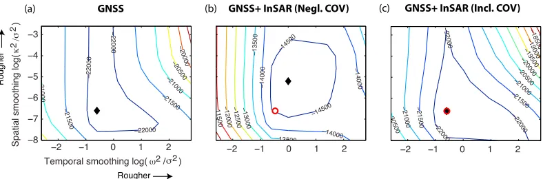
The NIF requires the specification of the hyperparameters for spatial and temporal smoothing. These can be selected through a maximum likelihood grid search, as proposed in the original NIF [Segall and Matthews, 1997], and applied in later studies [e.g.,Segall et al., 2000;Bartlow et al., 2011, 2014]. Unlike previous studies, we include both observations and pseudo observations in the computation of the maximum likelihood. Includ-ing the pseudo observations introduces a trade-off between fittInclud-ing the observations and smoothInclud-ing, which otherwise would not be included, leading to a higher likelihood for a rougher solution. Excluding pseudo observations would therefore lead to a rougher maximum likelihood solution. Once the hyperparameters have been selected, these can be ingested in a new NIF run.
2.5. Comparing the NIF With the Earlier Implementation
We modified the version of the NIF byBartlow et al.[2014], which works with GNSS data only, to include also InSAR data. While the main changes are related to the InSAR data component, we also include the interseis-mic rate directly in the inverse problem, whereasBartlow et al.[2014] correct the GNSS observations for the interseismic slip rate prior to ingestion in the NIF. To assess the impact of our modifications, we compared the results of our NIF version and that ofBartlow et al.[2014] when inverting GNSS observations of the 2011 Cascadia Slow Slip Event (SSE). This data set is distributed as test data for the earlier implementation of the NIF. Overall, we find that our implementation does not significantly alter the results obtained from the pre-vious implementation; average transient slip differences are<1 cm, and slip rate differences are negligible (∼0 cm/d).
3. Synthetic Simulation of the Guerrero SSE
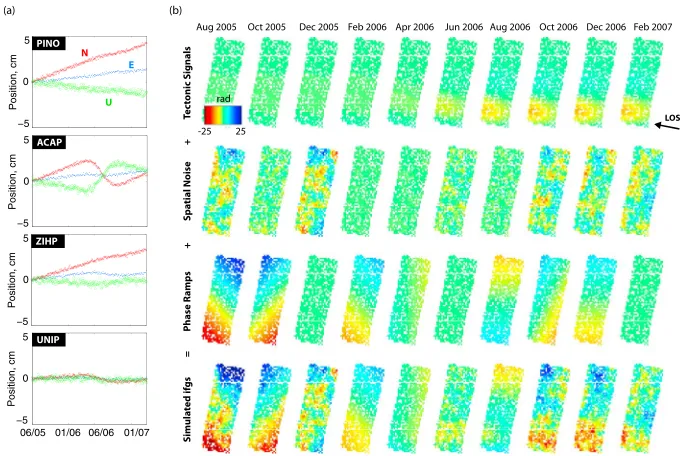
Our test data set reflects the tectonic setting in southern Mexico (Figure 1), with a simulation of the 2006 Guerrero SSE. Our observations span a duration of 1.8 years, from June 2005 to April 2007, and include an 8 month inter-SSE period, prior to the start of the 2006 SSE in February 2006 (1 year duration). We simulate the SSE, guided by the time-dependent GNSS modeling results ofRadiguet et al.[2011], who solved for the slow slip source time function. We adopt a similar source time parameterization scheme [Liu et al., 2006], where the location of slow slip initialization and the 0.8 km/d slip propagation velocity is from the best fit GNSS model byRadiguet et al.[2011]. For simplicity we fix the slow slip rise time, which is estimated to vary between 160 and 200 days [Radiguet et al., 2011], to be 183 days. For the maximum accumulated slip over the duration of the 2006 SSE, we use the results fromBekaert et al.[2015a], which are similar to other studies of the same event [e.g.,Vergnolle et al., 2010;Radiguet et al., 2011;Cavalié et al., 2013]. A full mathematical description of our time-dependent slow slip model as a function of the local slow slip start time, local rise time, and local cumulative slip magnitude is contained in Appendix B. Spatial maps of the local start time, rise time, and cumulative slip are shown in Figure S5 in the Supporting Information. We define the interseismic loading using a back slip formulation [Savage, 1983], where the slip deficit follows from the multiplication of the time with the MORVEL (Mid-Ocean Ridge VELocity) plate convergence rate of 6.1 cm/yr [DeMets et al., 2010] and a simulated inter-SSE coupling. The latter only varies with depth; we assume that the fault is freely slipping at shallow depths (coupling = 0), fully locked in the seismogenic zone between∼15 and 25 km (coupling = 1), and that there is a smooth transition region from 25 to 50 km depth, below which the fault is freely slipping.
Figure 1.Overview map of the Guerrero region, where the seven magenta triangles indicate the location of the continuous GNSS sites used in our simulation. Black triangles show the other GNSS stations of the network that were not considered. The red polygon shows the extent of the InSAR track. The gray arrow indicates the MORVEL (Mid-Ocean Ridge VELocity) relative plate motion of the Cocos and the North America Plate [DeMets et al., 2010], with depth contours of the subducting slab indicated every 20 km [Pardo and Suárez, 1995;Melgar and Pérez-Campos, 2011; Pérez-Campos and Clayton, 2014].
still solve for this in our NIF. A time series with the north, east, and up components is shown for selected GNSS stations in Figure 2a. The location of our simulated InSAR track corresponds to the location of the descend-ing Envisat track 255 (red polygon in Figure 1) used in earlier slow slip studies over the region [e.g.,Bekaert et al., 2015a;Cavalié et al., 2013]. We fix the master SAR acquisition to be on 1 June 2005, with a simulated SAR acquisition every 2 months. We generate 10 interferograms, and include orbit errors by simulating the addi-tion of a bilinear plane, for which the coefficients are summarized in Table 1. We incorporate the effects of
[image:7.612.203.544.470.698.2]Table 1.Parameters Used to Simulate InSAR Orbit Errorsaand Spatially Correlated Atmospheric InSAR Noiseb
𝛼 𝛽 𝛾 Lc 𝜎rn
Interferogram Dates (rad/km) (rad/km) (rad) (km) (rad)
1 Jun 2005 to 1 Aug 2005 0.1 0.1 1 50 6.73
1 Jun 2005 to 1 Oct 2005 −0.1 0.1 −1 10 2.24
1 Jun 2005 to 1 Dec 2005 0 0 0 40 6.73
1 Jun 2005 to 1 Feb 2006 0.05 0.05 0.1 1 0.22
1 Jun 2005 to 1 Apr 2006 −0.05 0 0 15 0.34
1 Jun 2005 to 1 Jun 2006 0 0 0 10 2.24
1 Jun 2005 to 1 Aug 2006 0 −0.05 0 5 1.12
1 Jun 2005 to 1 Oct 2006 −0.1 0.05 0 25 5.61
1 Jun 2005 to 1 Dec 2006 0 0.05 0 20 4.49
1 Jun 2005 to 1 Feb 2007 0 0 0 35 5.61
aOrbit errors are modeled as a bilinear plane according to[x 1,x2,1
] [𝛼, 𝛽, 𝛾]⊤.
bSpatially correlated noise is computed according to a method byLohman and Simons[2005], withL
cthe exponential range and𝜎rnthe standard deviation of the uncorrelated noise.
residual atmosphere delays by including spatially correlated noise according toLohman and Simons[2005], which varies in magnitude and correlation length for each interferogram as summarized in Table 1. Figure 2b shows the individually simulated components of the interferogram and the interferograms as input to the NIF. Our simulated interferograms have similar signal magnitude as processed Envisat data over the region [Bekaert et al., 2015a].
4. Results
We compare the NIF results when inverting for the GNSS observations only and when jointly inverting GNSS and InSAR observations. InSAR covariance is often neglected in slip inversion studies. This should be avoided as spatially correlated atmospheric noise will be treated as if it were a signal. The importance of covariance information has also been highlighted in other studies [e.g.,Lohman and Simons, 2005;Hetland et al., 2012;
Bekaert et al., 2015a;Agram and Simons, 2015;Fattahi and Amelung, 2015]. To demonstrate the impact of InSAR covariance on the estimated slip, we also include a comparison between results when the InSAR covariance is included in the inversion and when it is neglected. Our variance-covariance matrix is based on an exponential covariance function [Wackernagel, 2003] with the range and variance the same as those that were used when simulating the spatially correlated atmospheric noise (Table 1). We do not change the initialization of the state vector parameters between the different cases. Att =0, we assume the interseismic slip rate to be 0 cm/yr
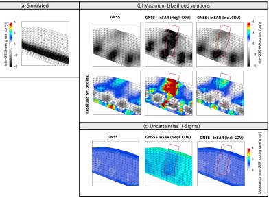
[image:8.612.179.573.545.675.2]Figure 4.Comparison of the inter-SSE locking rate. (a) The simulated rate, (b) the maximum likelihood solutions, and the residuals with respect to the simulated value. (c) Estimated uncertainties. We show the maximum likelihood solution when using GNSS alone, and the joint inversion with InSAR, while neglecting and accounting for the InSAR covariance information.
with a 6 cm/yr uncertainty, the accumulative slip to be 0 cm with a 1 cm uncertainty, and the transient slip rate to be 0 cm/d with an uncertainty of 10−8cm/d. These parameters are chosen assuming that the observations
start in an inter-SSE period. In our modeling we account only for reference frame translation (east, north, and up components). A priori knowledge of GNSS reference frame errors [e.g.,Wdowinski et al., 1997] and local station motion errors [e.g.,Dmitrieva et al., 2015] can be used to set their uncertainty in the NIF. However, we choose the reference frame uncertainty (1 mm) and local station motion uncertainty (1 mm yr−0.5) by trial
Figure 5.The same as Figure 4 but for the cumulative transient slip between January 2005 and April 2007.
hyperparameter grid search. However, after the maximum likelihood estimation (MLE) of the hyperparame-ters, we compute the MLE slip solution including the PDCO optimization. Below, we report on the results from the maximum likelihood solution for the three defined cases.
4.1. GNSS Only
Figure 3a shows the results of the hyperparameter grid search, with a maximum likelihood value for the spatial smoothing parameter of𝜅2∕𝜎2=24⋅10−8, temporal smoothing parameter of𝜔2∕𝜎2=0.24, and estimated
data variance-covariance scaling of̂𝜎=0.97. As expected, the latter is close to 1, indicating that the inversion is estimating the model to within expected errors. The results of the maximum likelihood solution after for-ward filtering and backfor-ward smoothing are shown in Figure 4 for the inter-SSE locking rate, Figure 5 for the cumulative estimated slow slip, and Figures 6–8 for the transient slip rate history.
The coastal GNSS stations are located approximately above the locked part of the subduction interface, Figure 4a, which is loaded in our simulation at a rate of∼6 cm/yr. We are capable of retrieving this same peak magnitude of 6 cm/yr. We find that the locking rate on the fault is well estimated for patches close to (∼20 km) the coastal GNSS sites, with a residual that falls within the∼1.5 cm/yr estimated uncertainty (Figure 4c). While a similar strike-parallel pattern can be observed, we find the peak distribution to be located∼10 km shallower than that in the input simulation. We observe some smearing farther downdip, with an average residual of
∼2.5 cm/yr, which is likely due to the imposed smoothing, to compensate for the overestimation near the trench. The poor resolution is not surprising given the very sparse GNSS coverage.
Our estimated cumulative slip, Figure 5b, is a smeared version of the simulation, Figure 5a. This is to be expected, as the GNSS network is not well distributed, with only the ACAP station clearly capturing the SSE surface displacements. We find the peak slip to be underestimated by∼7 cm, with an average estimated uncertainty of∼2 cm (Figure 5c). We also find some updip slip residuals introduced by the misestimation of the inter-SSE loading. The latter also causes the slip uncertainty to grow over time.
Figure 6.Transient slip rate history between January 2005 and April 2007, with a window each 2 months, averaged over∼70 days. The (first row) simulated slip rate is compared with the maximum likelihood solution when inverting for (second row) GNSS alone, (third row) the combination of GNSS and InSAR while neglecting InSAR covariance, and (fourth row) the joint inversion while including the InSAR covariance. The averaging duration is indicated above the panel as (+number of days).
simulation. On average, the transient slip rate is underestimated by∼0.06 cm/d during the transient period (Figure 7, first row). Uncertainties of our estimated transient slip rate are shown in Figure 8 (first row).
Figure 9 shows the variance and covariance history betweenv,W, andẆ (red line) for the triangular dis-location with peak slow slip and for another away from the slow slip region. As expected, we find that the interseismic slip rate is negatively correlated with the cumulative transient slip and transient slip rate. Halfway through the observation period, the covariance betweenvandẆ flattens. This could mean that oncevis well established by the pretransient data it does not trade off as much with transient slip. The correlation between
[image:11.612.95.518.545.703.2]vandWkeeps increasing (in absolute value) becauseWintegrates any uncertainty inẆ . The interseismic slip rate and its uncertainty are fixed based on the estimate from the last epoch and do not vary when performing the backward smoothing operation.
Figure 8.Uncertainty of the transient slip rate history when inverting for (first row) GNSS only, (second row) combining GNSS and InSAR while neglecting InSAR covariance, and the (third row) joint inversion while including the InSAR covariance. The panel averaging window is indicated above the panel as (+number of days).
Original observations and those estimated are shown in the Supporting Information (Figure S1). The modeled surface displacements fit the observations well, with a mean residual of around 0 mm and an accuracy similar to that of the simulated observations:∼1 mm for horizontal and∼2 mm for the vertical components.
4.2. GNSS and InSAR (Neglecting Covariance)
Figure 3b shows the results of the grid search for the hyperparameters. The estimated maximum like-lihood value for temporal smoothing hyperparameter (𝜔2∕𝜎2= 0.8) is double that of the GNSS case.
Compared to GNSS case, a much rougher spatial solution is preferred (𝜅2∕𝜎2=5⋅10−6). We find a lower value
for the estimated data variance-covariance scaling,̂𝜎=0.89, which implies that the model overfits the data.
As InSAR covariance information is not included, each of the∼103InSAR observations is treated as if it is an
independent observation. A much rougher solution is therefore found for the maximum likelihood solution. In reality much of this roughness is fitting the spatially correlated InSAR noise from the residual atmosphere. This results in apparent noise signals that propagate into the slip model. The estimated inter-SSE loading rate (Figure 4b) shows large residuals underneath the InSAR track, especially toward the downdip extent of the subduction interface (up to 8 cm/yr).
The cumulative transient peak slip is overestimated by∼3 cm, Figure 5b. Also, large errors relative to the true input slip with an average of∼12 cm can be observed at other locations, especially downdip of the slow slip region. Because the solution is rougher than the GNSS-only solution, we also find larger uncertainties for the estimated cumulative slip. The smallest uncertainty of∼4.5 cm can be found underneath the InSAR track and GNSS station locations, with larger values with an average of∼8 cm elsewhere.
The slip rate history (Figure 6, third row) shows much more temporal variation over the whole time period, even when there is no SSE taking place. These fluctuations reach an average magnitude of∼0.07 cm/d. Also, the corresponding uncertainties are larger than when inverting for GNSS alone (Figure 7, second row).
We find larger magnitudes for the variance and covariance history (blue line in Figure 9) than when using GNSS alone. We also observe a correlation between changes in the covariance history and those times when InSAR data were ingested into the NIF.
Figure 9.Time history of the variance and covariance of the interseismic slip rate (v), the cumulative transient slip (W), and the transient slip rate (Ẇ) for the two locations shown in the overview map. Location a) corresponds to the peak cumulative slow slip location, and location b) corresponds to a region away from the slow slip zone. The diagonal panels in Figures 9a and 9b show the time history of the variance forv,W, andẆ; while off-diagonal panels show the
covariance between each other. Red lines correspond to the NIF inversion when using only GNSS, blue when combining GNSS and InSAR while neglecting covariance, and green when GNSS and InSAR are combined including covariance information. Black solid lines represent the instants when an interferogram is formed. The dashed black line indicates the master acquisition of all interferograms.
orbital planes are well estimated with small residuals, average RMSE of∼0.7 rad (or 0.3 cm); see Supporting Information Figure S2b.
4.3. GNSS and InSAR (Including Covariance)
By including the full InSAR variance-covariance information, we find that the combined GNSS and InSAR solu-tion is more similar to the GNSS-only case. This is expected as the InSAR observasolu-tions add more informasolu-tion about the spatial extent of the slow slip surface observations. However, the InSAR contribution is down-weighted and provides only a lower level constraint [e.g.,Bekaert et al., 2015a], as the simulated slow slip signal has a correlation length similar to that of the simulated residual atmosphere (i.e.,∼2–50 km). By including the covariance, we find that the estimated data variance-covariance scaling is close to 1,̂𝜎=0.99. We also find similar hyperparameters to the GNSS-only case.
significant improvement in the location and estimation of the peak cumulative transient slip (Figure 5), misfit of<1 cm compared to∼7 cm for the GNSS-only case, and with a similar uncertainty of∼2 cm. The inter-SSE loading is slightly different to the GNSS case (Figure 4). We find a residual rate of up to 4.5 cm/yr underneath the InSAR track, downdip of the slow slip region. This is likely introduced to compensate for the smeared downdip slow slip signal. When neglecting InSAR covariance, this residual was significantly larger (up to∼8 cm/yr).
We find that the variance and covariance history (green line in Figure 9) tends more toward the GNSS case. However, a correlation can still be observed between the time of InSAR data ingestion and changes in the covariance history.
As before, we find small residuals for the GNSS and InSAR (Supporting Information Figure S3). GNSS residuals are within the uncertainty bounds of the simulated data. For the InSAR, we find the estimated tectonic signal and orbital errors with similar magnitudes as when neglecting the InSAR covariance. The misfit between the tectonic simulation and the estimation indicates underestimation of the slow slip signal.
5. Discussion
Our NIF results are a reasonable approximation of the simulated tectonic slow slip signal. We find that the InSAR observations provide an additional constraint on the slow slip signal at the fault interface, which is underestimated when inverting sparsely distributed GNSS observations only. After performing the backward smoothing, the NIF is capable of estimating the spatial variation of the transient slip rates at intervals shorter than the InSAR observations (see Supporting Information Figure S6). When comparing with our simulation, we find a similar transient slip rate nucleation zone (location difference<25 km). From visual inspection we find that our NIF results are capable of capturing the propagation of the slow slip over time. In general, we find the transient slip rates to be slightly smoother and consequently with a smaller peak magnitude than simulated. A more quantitative approach, which could be investigated in future studies, would be to parameterize the slip history for each of the dislocation patches and then to invert directly for the slow slip nucleation and propagation speed [e.g.,Radiguet et al., 2011].
Our NIF implementation is limited to a single spatial smoothing hyperparameter. We believe that it could be more appropriate to include a separate smoothing hyperparameter for the inter-SSE locking rate and also smooth differently in the dip and strike direction. For example, at subduction zones the interseismic slip rate is expected to vary with depth with a shorter wavelength than in the along-strike direction. Including an additional hyperparameter in our current NIF, implementation comes at the cost of an extra dimension to the grid search. In addition, but beyond the scope of our work, is the inclusion of model uncertainties due to, for example, fault geometry and elastic structure. For more information on how to handle these in a Bayesian framework see, for example,Duputel et al.[2014].
With a smaller grid spacing, and with more hyperparameters to solve for, the grid search becomes a time-consuming operation. An alternative approach to the grid search is included in the Extended NIF by
McGuire and Segall[2003], where the hyperparameters are included directly in the state vector. As in our study, the hyperparameters remain constant over time. Assuming that constant hyperparameters can be a limita-tion in a complex time series with a mixture of interseismic, coseismic, post seismic, aseismic, and slow slip processes. In particular, the rapid displacement change during a short-term SSE might be suppressed due to temporal smoothing. Developments byFukuda et al.[2004, 2008] allow for a time-varying temporal smooth-ing parameter. This is achieved by includsmooth-ing the temporal smoothsmooth-ing hyperparameter as stochastic variables using the Monte Carlo mixture Kalman filter or the hierarchical Bayesian state space approach. None of the above NIF modifications currently include InSAR capability. We believe that our presented methodology can be adopted straightforwardly into the other methods.
In our simulation, significant spatially correlated atmospheric noise (simulated variance between 1 and 3 cm2,
and correlation lengths up to 50 km) is added. InSAR covariance information is often neglected in tectonic slip inversion studies. This should be avoided, as spatially correlated noise will be treated as signal. This becomes of special importance in studies where the tectonic signals have a similar correlation length as the noise, as is the case for our simulation here. Recently, different efforts and promising progress have been made on the quantification and construction of InSAR variance-covariance matrices [e.g.,González and Fernández, 2011;
Agram and Simons, 2015;Fattahi and Amelung, 2015;Bekaert et al., 2015a]. Future modeling studies should aim to include InSAR covariance information as part of regular inversion procedures.
The quality of the InSAR observations is expected to improve with more regular SAR acquisitions. Our sim-ulation included a SAR acquisition every 60 days. With Sentinel 1 acquisitions are currently every 12 days, which will further decrease to every 6 days once Sentinel 1B is launched. With a swath width of∼250 km and a spatial resolution of 5×20m, large areas can be covered at high resolution and with short repeat times. Having a larger amount of independent InSAR observations will lead to a further reduction in the influence of atmospheric noise. In addition, atmospheric InSAR noise can be further reduced using tropospheric correc-tion methods [e.g.,Doin et al., 2009;Jolivet et al., 2011;Bekaert et al., 2015b, 2015c;Fattahi and Amelung, 2015]. Being able to ingest InSAR data for time-dependent modeling in the NIF could provide invaluable informa-tion in a variety of applicainforma-tions, such as volcano inflainforma-tion and deflainforma-tion, and fault creep, as well as coseismic and post seismic events.
6. Conclusions
Vast amounts of geodetic data have been acquired over the last two decades. The acquisition rate will continue to increase exponentially with further expansion of GNSS networks and the acquisition of InSAR data from Sentinel 1, NISAR, and ALOS 2. Simultaneous inversion of all geodetic data to solve for the time-dependent history of fault slip is a computationally intensive process, for which an alternative is the Network Inversion Filters. Different versions exist of this method, but to date, none of these include Interfer-ometric Synthetic Aperture (InSAR) observations. In this study, we have provided and applied the network inversion filter methodology to include InSAR. To validate the approach, we simulated the 2006 Guerrero SSE for a subset of the existing GNSS sites (mainly far field) and for the descending Envisat track 255. We find that GNSS can retrieve the cumulative SSE at approximately the same location as the input simulation, but with a smaller peak slip, due to spatial smoothing. Inclusion of high-resolution InSAR further improves the recov-ery of the transient slip. InSAR covariance is often neglected in slip inversion studies. This should be avoided, as spatially correlated atmospheric noise will be treated as if it was a signal, introducing apparent slip signals at depth. We compare the joint GNSS and InSAR inversion while neglecting and including InSAR covariance information. When including InSAR covariance, we find a solution that has similar smoothing hyperparame-ters to that of GNSS. We find that InSAR provides an improved constraint with its high-resolution observations above the slow slip region. Our study demonstrates the use of InSAR data to retrieve time-dependent slip, which can provide invaluable information for a wide variety of applications.
Appendix A: NIF Model for GNSS and Multiple InSAR Tracks
Here we expand the observation equation to include two InSAR tracks.
⎡ ⎢ ⎢ ⎢ ⎢ ⎢ ⎢ ⎢ ⎣ dGNSS ΔdInSAR,1 ΔdInSAR,2 0 0 0 ⎤ ⎥ ⎥ ⎥ ⎥ ⎥ ⎥ ⎥ ⎦tk
= ⎡ ⎢ ⎢ ⎢ ⎢ ⎢ ⎢ ⎢ ⎢ ⎣
GGNSS(t
k−t0GNSS
)
GGNSS 0 I F 0 0 0 0
GInSAR,1t
k GInSAR,1 0 0 0 PInSAR,1 −GInSAR,1 0 0
GInSAR,2t
k GInSAR,2 0 0 0 0 0 PInSAR,2 −GInSAR,2
𝛁2 0 0 0 0 0 0 0 0
0 𝛁2 0 0 0 0 0 0 0
0 0 𝛁2 0 0 0 0 0 0
⎤ ⎥ ⎥ ⎥ ⎥ ⎥ ⎥ ⎥ ⎥ ⎦t k ⏟⏞⏞⏞⏞⏞⏞⏞⏞⏞⏞⏞⏞⏞⏞⏞⏞⏞⏞⏞⏞⏞⏞⏞⏞⏞⏞⏞⏞⏞⏞⏞⏞⏞⏞⏞⏞⏞⏞⏞⏞⏞⏞⏞⏞⏞⏞⏞⏞⏞⏞⏞⏞⏞⏞⏞⏞⏞⏞⏞⏞⏞⏞⏟⏞⏞⏞⏞⏞⏞⏞⏞⏞⏞⏞⏞⏞⏞⏞⏞⏞⏞⏞⏞⏞⏞⏞⏞⏞⏞⏞⏞⏞⏞⏞⏞⏞⏞⏞⏞⏞⏞⏞⏞⏞⏞⏞⏞⏞⏞⏞⏞⏞⏞⏞⏞⏞⏞⏞⏞⏞⏞⏞⏞⏞⏞⏟ Hk ⎡ ⎢ ⎢ ⎢ ⎢ ⎢ ⎢ ⎢ ⎢ ⎢ ⎢ ⎢ ⎢ ⎢ ⎣ v W ̇ W InSAR,1
sInSAR,10
InSAR,2 sInSAR,20
⎤ ⎥ ⎥ ⎥ ⎥ ⎥ ⎥ ⎥ ⎥ ⎥ ⎥ ⎥ ⎥ ⎥ ⎦tk
+𝝐k,
Appendix B: Time-Dependent Slow Slip Simulation
FollowingLiu et al.[2006], we define the source time function of transient slip rate as
v=
⎧ ⎪ ⎨ ⎪ ⎩
As in(𝜋t tSSE
)
0≤t<tSSE∕2,
A
2
[
1+cos(2𝜋t tSSE−𝜋
)]
tSSE∕2≤t<tSSE (B1)
wheretis time,tSSEthe rise time and duration of the slow slip event, andAthe amplitude of the source func-tion. Here we assume that the acceleration and deceleration rise time have equal durafunc-tion. The time evolution of slip,s, follows from the integration of transient slip rate, where we define the integration constants andA
suchs=0att=tstartands=sSSE0 att=tSSE+tstart, leading to
s=
⎧ ⎪ ⎨ ⎪ ⎩
4sSSE 0
𝜋+4
[
1−cos(𝜋(t−tstart) tSSE
)]
tstart≤t<tSSE∕2+tstart
sSSE 0
𝜋+4
[2𝜋(t−t
start)
tSSE +4−𝜋−sin
(2𝜋(t−t
start) tSSE
)]
tSSE∕2+tstart≤t<tSSE+tstart
, (B2)
wheretstartis the start time of the slow slip event andsSSE
0 the cumulative slow slip. Equation (B2) defines
the slow slip evolution for an arbitrary location as a function of its local slow slip start time, rise time, and cumulative slip. An example of the time-dependant relation between slip rate and cumulative slip is contained in the Supporting Information Figure S4. Figure S5 gives the spatial maps of the local slow slip start time, rise time, and cumulative slip as input to our synthetic simulation.
Notation
InSAR Interferometric Synthetic Aperture Radar; GNSS Global Navigation Satellite System;
k+1∣k epochk+1given all data up to epochk;
k epochkgiven all data up to epochk; 𝛼, 𝛽, 𝛾 coefficients of the InSAR orbit error (plane);
𝜹 residual of state vector in the state transition equation;
𝝐GNSS,𝝐InSAR GNSS and InSAR observation errors;
GNSS reference frame coefficients (e.g., translation, rotation, and/or scaling); local GNSS benchmark motions for each component (ENU);
InSAR orbit (plane) coefficients ([𝛼, 𝛽, 𝛾]⊤); 𝛁2 Laplacian operator;
𝛀 s variance-covariance matrix;
I identity matrix;
O zero matrix;
R,𝚺 total and individual data set observation variance-covariance matrices;
Q process noise variance-covariance matrix;
ΔdInSAR InSAR radar line-of-sight surface displacements Δt time difference between epochs
̇
W slip rate or Random walk∼(0, 𝜔2);
𝜅 spatial smoothing parameter;
d observations of surface displacements;
F linearized Helmert transformation matrix of GNSS reference frame;
G Greens coefficients;
H observation matrix;
K Kalman filter gain;
P InSAR orbit (plane) matrix ([x1,x2,1
]
);
s fault slip;
sInSAR
0 reference slip at the InSAR reference time; T state transition matrix;
normal distribution;
𝜔 random walk-scale parameter controlling temporal smoothing; 𝜎 scaling parameter of the data observation variance-covariance matrix;
𝜏 scale parameter of the Brownian random walk of the local GNSS benchmark motion; 𝜁 scale parameter of the GNSS reference frame variance-covariance matrix;
Ns,Np,NI number of GNSS stations, InSAR pixels on a single track, and InSAR interferograms on a single track
tGNSS
0 ,tINSAR0 GNSS and InSAR reference time; t time;
v interseismic slip rate;
W integrated random walk or cumulative slip deviated from the steady state interseismic slip rate;
References
Agram, P. S., and M. Simons (2015), A noise model for InSAR time series,J. Geophys. Res. Solid Earth,120, 2752–2771, doi:10.1002/2014JB011271.
Bartlow, N. M., S. Miyazaki, A. M. Bradley, and P. Segall (2011), Space-time correlation of slip and tremor during the 2009 Cascadia slow slip event,Geophys. Res. Lett.,38, L18309, doi:10.1029/2011GL048714.
Bartlow, N. M., L. M. Wallace, R. J. Beavan, S. Bannister, and P. Segall (2014), Time-dependent modeling of slow slip events and associated seismicity and tremor at the Hikurangi subduction zone, New Zealand,J. Geophys. Res. Solid Earth,119, 734–753, doi:10.1002/2013JB010609.
Bedford, J., et al. (2013), A high-resolution, time-variable afterslip model for the 2010 Maule Mw = 8.8, Chile megathrust earthquake,
Earth Planet. Sci. Lett.,383, 26–36, doi:10.1016/j.epsl.2013.09.020.
Bekaert, D., A. Hooper, and T. Wright (2015a), Reassessing the 2006 Guerrero slow slip event, Mexico: Implications for large earthquakes in the Guerrero Gap,J. Geophys. Res. Solid Earth,120, 1357–1375, doi:10.1002/2014JB011557.
Bekaert, D., A. Hooper, and T. Wright (2015b), A spatially-variable power-law tropospheric correction technique for InSAR data,
J. Geophys. Res. Solid Earth,120, 1345–1356, doi:10.1002/2014JB011558.
Bekaert, D., R. Walters, T. Wright, A. Hooper, and D. Parker (2015c), Statistical comparison of InSAR tropospheric correction techniques,
Remote Sens. Environ.,170, 40–47, doi:10.1016/j.rse.2015.08.035.
Cavalié, O., E. Pathier, M. Radiguet, M. Vergnolle, N. Cotte, A. Walpersdorf, V. Kostoglodov, and F. Cotton (2013), Slow slip event in the Mexican subduction zone: Evidence of shallower slip in the Guerrero seismic gap for the 2006 event revealed by the joint inversion of InSAR and GPS data,Earth and Planet. Sci. Lett.,367, 52–60, doi:10.1016/j.epsl.2013.02.020.
Cervelli, P., P. Segall, K. Johnson, M. Lisowski, and A. Miklius (2002), Sudden aseismic fault slip on the south flank of Kilauea volcano,Nature,
414(6875), 1014–1018, doi:10.1038/4151014a.
DeMets, C., R. Gordon, and D. Argus (2010), Geologically current plate motions,Geophys. J. Int.,181(1), 1–80, doi:10.1111/j.1365-246X.2009.04491.x.
Dmitrieva, K., P. Segall, and C. DeMets (2015), Network-based estimation of time-dependent noise in GPS position time series,J. Geod.,89(6), 591–606, doi:10.1007/s00190-015-0801-9.
Doin, M., C. Lasserre, G. Peltzer, O. Cavalié, and C. Doubre (2009), Corrections of stratified tropospheric delays in SAR interferometry: Validation with global atmospheric models,J. Appl. Geophys.,69(1), 35–50, doi:10.1016/j.jappgeo.2009.03.010.
Duputel, Z., P. S. Agram, M. Simons, S. E. Minson, and J. L. Beck (2014), Accounting for prediction uncertainty when inferring subsurface fault slip,Geophys. J. Int.,197(1), 464–482, doi:10.1093/gji/ggt517.
Fattahi, H., and F. Amelung (2015), InSAR bias and uncertainty due to the systematic and stochastic tropospheric delay,J. Geophys. Res. Solid Earth,120, 8758–8773, doi:10.1002/2015JB012419.
Fukuda, J., T. Higuchi, S. Miyazaki, and T. Kato (2004), A new approach to time-dependent inversion of geodetic data using a Monte Carlo mixture Kalman filter,Geophys. J. Int.,159(1), 17–39, doi:10.1111/j.1365-246X.2004.02383.x.
Fukuda, J., S. Miyazaki, T. Higuchi, and T. Kato (2008), Geodetic inversion for space-time distribution of fault slip with time-varying smoothing regularization,Geophys. J. Int.,173(1), 25–48, doi:10.1111/j.1365-246X.2007.03722.x.
González, P. J., and J. Fernández (2011), Error estimation in multitemporal InSAR deformation time series, with application to Lanzarote, Canary Islands,J. Geophys. Res.,116, B10404, doi:10.1029/2011JB008412.
Hetland, E. A., P. Musé, M. Simons, Y. N. Lin, P. S. Agram, and C. J. DiCaprio (2012), Multiscale InSAR Time Series (MInTS) analysis of surface deformation,J. Geophys. Res.,117, B02404, doi:10.1029/2011JB008731.
Hooper, A., D. Bekaert, K. Spaans, and M. Arikan (2012), Recent advances in SAR interferometry time series analysis for measuring crustal deformation,Tectonophysics,514–517, 1–13, doi:10.1016/j.tecto.2011.10.013.
Hsu, Y.-J., M. Simons, J.-P. Avouac, J. Galetzka, K. Sieh, M. Chlieh, D. Natawidjaja, L. Prawirodirdjo, and Y. Bock (2006), Frictional afterslip following the 2005 Nias-Simeulue earthquake, Sumatra,Science,312(5782), 1921–1926, doi:10.1126/science.1126960.
Jolivet, R., R. Grandin, C. Lasserre, M. Doin, and G. Peltzer (2011), Systematic InSAR tropospheric phase delay corrections from global meteorological reanalysis data,Geophys. Res. Lett.,38, L17311, doi:10.1029/2011GL048757.
Jónsson, S., H. Zebker, P. Segall, and F. Amelung (2002), Fault slip distribution of the 1999 Mw 7.1 hector mine, California, earthquake, estimated from satellite radar and GPS measurements,Bull. Seismol. Soc. Am.,92(4), 1377–1389, doi:10.1785/0120000922. Kositsky, A. P., and J.-P. Avouac (2010), Inverting geodetic time series with a principal component analysis-based inversion method,
J. Geophys. Res.,115, B03401, doi:10.1029/2009JB006535.
Langbein, J., and H. Johnson (1997), Correlated errors in geodetic time series: Implications for time-dependent deformation,
J. Geophys. Res.,102(B1), 591–603, doi:10.1029/96JB02945.
Liu, P., S. Custódio, and R. J. Archuleta (2006), Kinematic inversion of the 2004 M 6.0 Parkfield earthquake including an approximation to site effects,Bull. Seismol. Soc. Am.,96(4B), 143–158, doi:10.1785/0120050826.
Lohman, R. B., and M. Simons (2005), Some thoughts on the use of InSAR data to constrain models of surface deformation: Noise structure and data downsampling,Geochem. Geophys. Geosyst.,6, Q01007, doi:10.1029/2004GC000841.
Acknowledgments
Mavrommatis, A. P., P. Segall, and K. M. Johnson (2014), A decadal-scale deformation transient prior to the 2011 Mw 9.0 Tohoku-oki earthquake,Geophys. Res. Lett.,41, 4486–4494, doi:10.1002/2014GL060139.
McGuire, J. J., and P. Segall (2003), Imaging of aseismic fault slip transients recorded by dense geodetic networks,Geophys. J. Int.,155(3), 778–788, doi:10.1111/j.1365-246X.2003.02022.x.
Melgar, D., and X. Pérez-Campos (2011), Imaging the moho and subducted oceanic crust at the isthmus of Tehuantepec, Mexico, from receiver functions,Pure Appl. Geophys.,168(8–9), 1449–1460, doi:10.1007/s00024-010-0199-5.
Miyazaki, S., J. J. McGuire, and P. Segall (2003), A transient subduction zone slip episode in Southwest Japan observed by the nationwide GPS array,J. Geophys. Res.,108(B2), 2087, doi:10.1029/2001JB000456.
Miyazaki, S., P. Segall, J. Fukuda, and T. Kato (2004), Space time distribution of afterslip following the 2003 Tokachi-oki earthquake: Implications for variations in fault zone frictional properties,J. Geophys. Res.,31, L06623, doi:10.1029/2003GL019410.
Okada, Y. (1985), Surface deformation due to shear and tensile faults in a half-space,Bull. Seismol. Soc. Am.,75(4), 1135–1154. Ozawa, S., H. Suito, T. Imakiire, and M. Murakmi (2007), Spatiotemporal evolution of aseismic interplate slip between 1996 and 1998 and
between 2002 and 2004, in Bungo Channel, Southwest Japan,J. Geophys. Res.,112, B05409, doi:10.1029/2006JB004643.
Pardo, M., and G. Suárez (1995), Shape of the subducted Rivera and Cocos Plates in southern Mexico: Seismic and tectonic implications,
J. Geophys. Res.,100(B7), 12,357–12,373, doi:10.1029/95JB00919.
Pérez-Campos, X., and R. W. Clayton (2014), Interaction of Cocos and Rivera plates with the upper-mantle transition zone underneath Central Mexico,Geophys. J. Int.,197(3), 1763–1769, doi:10.1093/gji/ggu087.
Pritchard, M. E., M. Simons, P. A. Rosen, S. Hensley, and F. H. Webb (2002), Co-seismic slip from the 1995 July 30 Mw = 8.1 Antofagasta, Chile, earthquake as constrained by InSAR and GPS observations,Geophys. J. Int.,150(2), 362–376, doi:10.1046/j.1365-246X.2002.01661.x. Radiguet, M., F. Cotton, M. Vergnolle, M. Campillo, B. Valette, V. Kostoglodov, and N. Cotte (2011), Spatial and temporal evolution of a long
term slow slip event: The 2006 Guerrero Slow Slip Event,Geophys. J. Int.,184(2), 816–828, doi:10.1111/j.1365-246X.2010.04866.x. Rauch, H., C. Striebel, and F. Tung (1965), Maximum likelihood estimates of linear dynamic systems,Am. Inst. Aeronaut. Astronaut. J.,3(8),
1445–1450, doi:10.2514/3.3166.
Saunders, M. (2015),PDCO Convex Optimization Software, Stanford, Calif. [Available at http://web.stanford.edu/group/SOL/software/pdco/.] Savage, J. C. (1983), A dislocation model of strain accumulation and release at a subduction zone,J. Geophys. Res.,88(B6), 4984–4996,
doi:10.1029/JB088iB06p04984.
Schmidt, D. A., and H. Gao (2010), Source parameters and time-dependent slip distributions of slow slip events on the Cascadia subduction zone from 1998 to 2008,J. Geophys. Res.,115, B00A18, doi:10.1029/2008JB006045.
Segall, P., and M. Matthews (1997), Time dependent inversion of geodetic data,J. Geophys. Res.,102(B10), 22,391–22,409, doi:10.1029/97JB01795.
Segall, P., R. Bürgmann, and M. Matthews (2000), Time-dependent triggered afterslip following the 1989 Loma Prieta earthquake,
J. Geophys. Res.,105(B3), 5615–5634, doi:10.1029/1999JB900352.
Segall, P., E. K. Desmarais, D. Shelly, A. Miklius, and P. Cervelli (2006), Earthquakes triggered by silent slip events on Kilauea volcano, Hawaii,
Nature,442(7098), 71–74, doi:10.1038/nature04938.
Shirzaei, M., and R. Burgmann (2013), Time-dependent model of creep on the Hayward fault from joint inversion of 18 years of InSAR and surface creep data,J. Geophys. Res.,118(4), 1733–1746, doi:10.1002/jgrb.50149.
Shirzaei, M., and T. R. Walter (2010), Time-dependent volcano source monitoring using interferometric synthetic aperture radar time series: A combined genetic algorithm and Kalman filter approach,J. Geophys. Res.,115, B10421, doi:10.1029/2010JB007476.
Simon, D., and D. L. Simon, (2010), Constrained Kalman filtering via density function truncation for turbofan engine health estimation,Int. J. Syst. Sci.,41(2), 159–171, doi:10.1080/00207720903042970.
Simons, M., Y. Fialko, and L. Rivera (2002), Coseismic deformation from the 1999 Mw 7.1 Hector mine, California, earthquake as inferred from InSAR and GPS observations,Bull. Seismol. Soc. Am.,92(4), 1390–1402, doi:10.1785/0120000933.
Thomas, A. (1993), Poly3D: A three-dimensional, polygonal element, displacement discontinuity boundary element computer pro-gram with applications to fractures, faults and cavities in the Earth’s crust, Master’s thesis, Stanford Univ., Stanford, Calif. [Available at https://earthsciences.stanford.edu/research/geomech/Software/academic/doc/Thomas_thesis.pdf.]
Vergnolle, M., A. Walpersdorf, V. Kostoglodov, P. Tregoning, J. Santiago, N. Cotte, and S. Franco (2010), Slow slip events in Mexico revised from the processing of 11-year GPS observations,J. Geophys. Res.,115, B08403, doi:10.1029/2009JB006852.
Wackernagel, H. (Ed.) (2003),Multivariate Geostatistics, 3rd ed., Springer, Berlin.
Wdowinski, S., Y. Bock, J. Zhang, P. Fang, and J. Genrich (1997), Southern California permanent GPS geodetic array: Spatial filtering of daily positions for estimating coseismic and postseismic displacements induced by the 1992 landers earthquake,J. Geophys. Res.,102(B8), 18,057–18,070, doi:10.1029/97JB01378.
Wessel, P., and W. Smith (1991), Free software helps map and display data,Eos Trans. AGU,72(41), 445–446, doi:10.1029/90EO00319. Wright, T., Z. Lu, and C. Wicks (2004), Constraining the slip distribution and fault geometry of the Mw 7.9, 3 November 2002, Denali fault