https://doi.org/10.5194/gmd-10-4035-2017 © Author(s) 2017. This work is distributed under the Creative Commons Attribution 3.0 License.
The PMIP4 contribution to CMIP6 – Part 4: Scientific objectives
and experimental design of the PMIP4-CMIP6 Last Glacial
Maximum experiments and PMIP4 sensitivity experiments
Masa Kageyama1, Samuel Albani1, Pascale Braconnot1, Sandy P. Harrison2, Peter O. Hopcroft3, Ruza F. Ivanovic4, Fabrice Lambert5, Olivier Marti1, W. Richard Peltier6, Jean-Yves Peterschmitt1, Didier M. Roche1,7, Lev Tarasov8, Xu Zhang9, Esther C. Brady10, Alan M. Haywood4, Allegra N. LeGrande11, Daniel J. Lunt3, Natalie M. Mahowald12, Uwe Mikolajewicz13, Kerim H. Nisancioglu14,15, Bette L. Otto-Bliesner10, Hans Renssen7,16, Robert A. Tomas10, Qiong Zhang17, Ayako Abe-Ouchi18, Patrick J. Bartlein19, Jian Cao20, Qiang Li17, Gerrit Lohmann9,
Rumi Ohgaito18,21, Xiaoxu Shi9, Evgeny Volodin22, Kohei Yoshida23, Xiao Zhang24,25, and Weipeng Zheng26 1Laboratoire des Sciences du Climat et de l’Environnement, LSCE/IPSL, CEA-CNRS-UVSQ, Université Paris-Saclay, 91191 Gif-sur-Yvette, France
2Centre for Past Climate Change and School of Archaeology, Geography and Environmental Science (SAGES) University of Reading, Whiteknights, Reading, RG6 6AH, UK
3School of Geographical Sciences, University of Bristol, Bristol, BS8 1SS, UK 4School of Earth and Environment, University of Leeds, Leeds, LS2 9JT, UK
5Department of Physical Geography, Pontifical Catholic University of Chile, Santiago, Chile
6Department of Physics, University of Toronto, 60 St. George Street, Toronto, Ontario M5S 1A7, Canada 7Earth and Climate Cluster, Faculty of Earth and Life Sciences, Vrije Universiteit Amsterdam,
Amsterdam, the Netherlands
8Department of Physics and Physical Oceanography, Memorial University of Newfoundland and Labrador, St. John’s, NL, A1B 3X7, Canada
9Alfred Wegener Institute Helmholtz Centre for Polar and Marine Research, Bussestrasse 24, 27570, Bremerhaven, Germany
10National Center for Atmospheric Research, 1850 Table Mesa Drive, Boulder, CO 80305, USA 11NASA Goddard Institute for Space Studies, 2880 Broadway, New York, NY 10025, USA
12Department of Earth and Atmospheric Sciences, Bradfield 1112, Cornell University, Ithaca, NY 14850, USA 13Max Planck Institute for Meteorology, Bundesstrasse 53, 20146 Hamburg, Germany
14Department of Earth Science, University of Bergen and the Bjerknes Centre for Climate Research, Allégaten 41, 5007 Bergen, Norway
15Department of Geosciences and the Centre for Earth Evolution and Dynamics, University of Oslo, Sem Sælands vei 2A, 0371 Oslo, Norway
16Department of Natural Sciences and Environmental Health, University College of Southeast Norway, Bø, Norway 17Department of Physical Geography, Stockholm University and Bolin Centre for Climate Research,
Stockholm, Sweden
18Atmosphere Ocean Research Institute, University of Tokyo, 5-1-5, Kashiwanoha, Kashiwa-shi, Chiba 277-8564, Japan
19Department of Geography, University of Oregon, Eugene, OR 97403-1251, USA
20Earth System Modeling Center, Nanjing University of Information Science and Technology, Nanjing, China
21Japan Agency for Marine-Earth Science and Technology, Yokohama, Japan
24School of Atmospheric Science, Nanjing University of Information sciences and Technology, Nanjing, 210044, China
25International Pacific Research Center, University of Hawaii at Manoa, Honolulu, HI 96822, USA
26State Key Laboratory of Numerical Modeling for Atmospheric Sciences and Geophysical Fluid Dynamics (LASG), Institute of Atmospheric Physics, Chinese Academy of China, 100029, Beijing, China
Correspondence to:Masa Kageyama ([email protected]) Received: 26 January 2017 – Discussion started: 23 February 2017
Revised: 12 July 2017 – Accepted: 24 July 2017 – Published: 7 November 2017
Abstract. The Last Glacial Maximum (LGM, 21 000 years ago) is one of the suite of paleoclimate simulations included in the current phase of the Coupled Model Intercompari-son Project (CMIP6). It is an interval when insolation was similar to the present, but global ice volume was at a maxi-mum, eustatic sea level was at or close to a minimaxi-mum, green-house gas concentrations were lower, atmospheric aerosol loadings were higher than today, and vegetation and land-surface characteristics were different from today. The LGM has been a focus for the Paleoclimate Modelling Intercom-parison Project (PMIP) since its inception, and thus many of the problems that might be associated with simulating such a radically different climate are well documented. The LGM state provides an ideal case study for evaluating cli-mate model performance because the changes in forcing and temperature between the LGM and pre-industrial are of the same order of magnitude as those projected for the end of the 21st century. Thus, the CMIP6 LGM experiment could pro-vide additional information that can be used to constrain es-timates of climate sensitivity. The design of the Tier 1 LGM experiment (lgm) includes an assessment of uncertainties in boundary conditions, in particular through the use of differ-ent reconstructions of the ice sheets and of the change in dust forcing. Additional (Tier 2) sensitivity experiments have been designed to quantify feedbacks associated with land-surface changes and aerosol loadings, and to isolate the role of individual forcings. Model analysis and evaluation will capitalize on the relative abundance of paleoenvironmental observations and quantitative climate reconstructions already available for the LGM.
1 Introduction
The Last Glacial Maximum (LGM), dated ∼21 000 years BP, is the last period during which the global ice volume was at its maximum, and eustatic sea level at or near to its minimum,∼115 to 130 m below the present sea level (Lam-beck et al., 2014; Peltier and Fairbanks, 2006). It has been defined as a relatively stable climatic period, in between two major intervals of iceberg discharge into the North Atlantic, Heinrich events 1 and 2 (Mix et al., 2001). In addition to
Dry conditions and the reduction in vegetation cover led to major changes in dust emission, recorded in ice cores, ma-rine sediments, and loess/paleosol deposits. Based on global compilations of these records, it has been estimated that the LGM was 2–4 times dustier than the Holocene on global average (Kohfeld and Harrison, 2001; Maher et al., 2010). However, the spatial variability of changes in dust deposition rates is very large, with a 20-fold increase shown in polar ice cores (Lambert et al., 2008; Steffensen et al., 2008). These changes in dust loading reflect changes in surface character-istics, winds, and precipitation. They also represent an im-portant feedback from the climate system onto atmospheric radiative properties, which include direct and indirect effects on the atmospheric radiation budget through scattering and absorption of radiation and dust-cloud interactions (Boucher et al., 2013), which can alter regional climates (Claquin et al., 2003; Mahowald et al., 2006; Takemura et al., 2009; Hopcroft et al., 2015). Dust deposition changes can also im-pact the global carbon cycle, in particular because of the po-tential fertilization effect that dust-borne iron may exert on the Southern Ocean marine ecosystems and carbon seques-tration in the deep ocean (Martin et al., 1990; Bopp et al., 2003; Kohfeld et al., 2005).
Modelling the LGM climate has been a focus for the Pa-leoclimate Modelling Intercomparison Project (PMIP) since its beginning (Joussaume and Taylor, 1995), progressing from simulations with atmospheric general circulation mod-els (AGCMs), using prescribed ocean conditions or coupled to slab ocean models, to simulations using fully coupled atmosphere–ocean general circulation models (AOGCMs), some of which included vegetation dynamics, in the sec-ond phase of PMIP (PMIP2: Braconnot et al., 2007), and Earth system models (ESMs) with interactive carbon cycles in PMIP’s third phase (PMIP3: Braconnot et al., 2012). The progression from AGCMs to AOGCMs has allowed oceanic reconstructions to be used for model evaluation and analy-sis of the physical conanaly-sistency (as represented by models) of continental and oceanic reconstructions (e.g. Kageyama et al., 2006). At each phase in this evolution, PMIP has taken into account new knowledge about boundary conditions, in particular for the form of the ice sheets, as well as the new ca-pabilities of climate models. This paper describes the exper-imental set-up for the LGM experiments for PMIP4-CMIP6. Compared to the previous phases of PMIP, the new aspects of the PMIP4-CMIP6 simulations are
– the inclusion of dust forcing, either by using models in which the dust cycle is interactive or by prescribing at-mospheric dust concentrations, so as to consider the in-teractions between dust and radiation. This is expected to cause significant differences in simulated regional cli-mates and to have impacts on ocean biogeochemistry through a more realistic representation of dust input at the ocean surface; and
– explicit consideration of the uncertainties in ice-sheet reconstructions and the impact of different reconstruc-tions of ice-sheet elevation on simulated climate. Con-sideration of uncertainties in boundary conditions is particularly important when comparing the model re-sults to paleoclimatic reconstructions and drawing con-clusions about the capabilities of the state-of-the-art models that are used for future climate projections. This paper provides guidelines on the implementation of the PMIP4 LGM experiment in the CMIP6 climate models. This LGM experiment is a Tier 1 CMIP6 experiment (as defined in Eyring et al., 2016, i.e. Tier 1 defines experiments with the highest priority) and one of the two possible entry cards for PMIP4 (Kageyama et al., 2016). It is also a reference exper-iment for additional sensitivity experexper-iments, which are con-sidered Tier 2 and described here. These additional experi-ments are designed to improve our understanding of the sim-ulated LGM climate. Section 2 presents how the LGM exper-iment will address CMIP6 questions. Section 3 describes the LGM PMIP4-CMIP6 experiments and the PMIP4 sensitivity experiments that were designed to address these questions. Section 4 details the implementation of LGM simulations. Section 5 finally outlines the analysis plan of the LGM exper-iments. There are two companion papers which document the other PMIP4-CMIP6 experiments: the last interglacial and mid-Holocene (Otto-Bliesner et al., 2017) and the last mil-lennium (Jungclaus et al., 2017). In addition, Kageyama et al. (2016) provide an overview of the PMIP4-CMIP6 project.
2 The relevance of the LGM experiment for CMIP6 The LGM experiments are directly relevant to CMIP6 ques-tions 1 and 2 (Eyring et al, 2016): “How does the Earth Sys-tem respond to forcing?”, and “What are the origins and con-sequences of systematic model biases?”.
1. What are the responses of the Earth system to the LGM forcings?
in climate above and around the ice sheets (e.g. Löfver-ström et al., 2014, 2016), but also at a larger scale if the changes in large-scale circulation are sufficiently large to have an impact on the North Atlantic Ocean circu-lation (e.g. Roberts et al., 2014; Ullman et al., 2014; Zhang et al., 2014; Beghin et al., 2016). Several stud-ies have shown that changes in vegetation cover and in-creases in dust loading affect LGM climates (e.g. Ma-her et al., 2010; Albani et al., 2014). The design of the PMIP4-CMIP6 simulations allows the impact of vegeta-tion and dust forcing to be explored systematically. The Tier 2 PMIP4 sensitivity experiments will separate the influence of individual forcings (GHG and ice sheets) on the LGM climate. Thus, the PMIP4-CMIP6 Tier 1 LGM experiment, and the associated Tier 2 sensitiv-ity experiments, will help to understand the response to multiple forcings, the sensitivity to individual forcings, and how the responses to individual features and forc-ings combine to produce the full LGM response. 2. Can models represent the reconstructed climatic and
en-vironmental changes for the LGM?
Model evaluation based on LGM climate or environ-mental reconstructions has been an ongoing activity since the beginning of PMIP (Braconnot et al., 2012; Harrison et al., 2014, 2015; Annan and Hargreaves, 2015). Model–data comparisons have been performed at data sites and this has helped identify discrepancies in the LGM experimental set-up (e.g. for the eastward extension of the Fennoscandian ice sheet which had a strong impact on summer temperatures, Kageyama et al., 2006). Data–model comparison has helped to es-tablish the realism of large-scale climatic features, such as polar amplification, land–sea contrast and precipita-tion scaling with temperature (Masson-Delmotte et al., 2006; Izumi et al., 2013; Li et al., 2013; Lambert et al., 2013; Schmidt et al., 2014), and the ocean state and deep circulation (e.g. Otto-Bliesner et al., 2007; Muglia and Schmittner, 2015; Zhang et al., 2013). Benchmark-ing in comparison to paleoclimatic surface reconstruc-tions (land and ocean) has shown there has been lit-tle improvement from PMIP2 to PMIP3, especially at the regional scale (Harrison et al., 2014; Annan and Hargreaves, 2015). However, in PMIP4, given improve-ments in the climate models themselves, the inclusion of additional boundary conditions (dust, vegetation) and updates to pre-existing boundary conditions (e.g. ice sheets, river routing, GHGs) in line with latest knowl-edge, the simulations of regional climate should be more realistic. In addition, models now explicitly rep-resent processes or climate system components such as marine biogeochemistry, oxygen and carbon isotopes, dust emission and transport, and vegetation dynamics, making it possible to make direct comparisons with en-vironmental records and reducing the uncertainties
re-sulting from the interpretation of these records in terms of climate signals in model–data comparisons. An im-portant aspect of the data–model comparisons will be to determine whether there is sufficient data to charac-terize and quantify differences in regional climates re-sulting from the uncertainties in the imposed boundary conditions (i.e. different ice sheets, different representa-tions of vegetation and/or dust forcing).
3. What are the roles of each component of the climate sys-tem, or of specific processes within the climate syssys-tem, in producing the LGM climate?
The LGM climate is the result of a combined set of forc-ings and feedbacks. In particular, decreased GHG and increased dust act on the atmospheric radiative forcings and feedbacks; changes in sea ice provide a feedback to atmospheric radiation, atmosphere–ocean exchanges, and ocean circulation (deep water formation); the ice sheets and vegetation changes act on the albedo and surface energy fluxes; ice-sheet topography, decreased sea level, and modified bathymetry act on the spheric and oceanic circulations; the decreased atmo-spheric CO2 concentration acts on vegetation and the way it exchanges water and CO2with the atmosphere via changes in water-use efficiency. Thus, much can be learnt about the respective role and magnitude of key feedbacks affecting Earth’s energetics by analysing the PMIP4-CMIP6 LGM experiments, as well as the PMIP4 sensitivity experiments. These were developed following a few studies led with single models (e.g. Klockmann et al., 2016; Brady et al., 2013; Pausata et al., 2011). We also expect analyses of the impacts of these LGM forcings to strongly benefit from diagnostics developed by the Modelling Intercomparison Projects (MIPs) dedicated to these components and processes, such as OMIP for the ocean (Griffies et al., 2016; Orr et al., 2017), SIMIP for sea-ice processes (Notz et al., 2016), LS3MIP for the land surface (van den Hurk et al., 2016), AerChemMIP for dust (Collins et al., 2017), CFMIP for clouds (Webb et al., 2017), and RFMIP for radiative forcing diagnostics (Pincus et al., 2016). 4. Can the LGM climate constrain climate sensitivity?
re-constructions of these tropical SSTs, which have been strongly debated since CLIMAP (1981) and still show discrepancies (as summarized in e.g. Annan and Har-greaves, 2015). On the other hand, the studies using CMIP-type models have shown that more individual simulations than presently available are required to es-tablish statistically significant relationships. Analysis of the processes involved in the temperature response to the forcings (i.e. GHG for current-to-future warming, and ice sheets and GHG for the LGM-to-pre-industrial warming) are essential for this investigation, because while some feedbacks appear to work in a similar man-ner for LGM-to-pre-industrial and for future warming, feedbacks such as the cloud radiative feedback do not (Yoshimori et al., 2009). The relative magnitudes of the different feedbacks also vary between those two cli-mates, so that the relationship with climate sensitiv-ity is not straightforward (Braconnot and Kageyama, 2015). Changes in vegetation and dust, which produce changes in regional climate, also need to be taken into account when regional reconstructions (such as over the tropical oceans) are used to constrain climate sen-sitivity (Hopcroft and Valdes, 2015a). By increasing the number of simulations available, including impor-tant regional forcings, and focusing on uncertainties in these forcings, the LGM PMIP4-CMIP6 experiments will provide a much better data set to re-examine cli-mate sensitivity.
3 PMIP4-CMIP6 experiments and PMIP4 sensitivity experiments
This section describes the PMIP4-CMIP6 Tier 1 LGM cli-mate experiment, termed “lgm”, as well as complementary PMIP4 Tier 2 sensitivity experiments. These are also sum-marized in Table 1. Section 4 describes how to implement the associated boundary conditions.
3.1 The Tier 1 PMIP4-CMIP6lgmexperiment
The lgmsimulation is a CMIP6 Tier 1 experiment, as well as one of the two possible PMIP4 entry cards (i.e. one of the two simulations that must be performed by modelling groups wishing to officially take part in PMIP4). Thelgmsimulation will be compared to the CMIP DECK (Diagnostic, Evalu-ation and CharacterizEvalu-ation of Klima) pre-industrial control (piControl) for 1850 CE and the CMIP6historical experi-ment (Eyring et al., 2016) and must therefore be run using the same version (including level of complexity and the in-teractive feedbacks) and resolution of the model and follow-ing the same protocols for implementfollow-ing external forcfollow-ings as in these two reference simulations.
The minimum set of changes that must be made for the lgm simulation, compared to the set-up of the piControl,
are the insolation, GHG, and ice-sheet forcings (see Sect. 4 for the implementation of these changes). There are several plausible alternatives for the ice-sheet forcing and modelling groups can choose between one of three options (Fig. 1): the ice-sheet reconstruction produced for PMIP3 (Abe-Ouchi et al., 2015), the ICE-6G_C reconstruction (Peltier et al., 2015; Argus et al., 2014), or the GLAC-1D (Tarasov et al., 2012; Briggs et al., 2014; Ivanovic et al., 2016). However, if the PMIP4 transient last deglaciation experiment is run (Ivanovic et al., 2016), the modelling groups should ensure consistency between the LGM simulation and subsequent transient phase of the experiment, when possible.
The dust and vegetation forcing in the Tier 1lgm experi-ment must be imposed in a manner that is consistent with the DECK simulations. Models that include interactive dust, for example, should allow interactive emissions at the LGM. For this purpose, two alternative reconstructions of LGM dust emission regions are provided for models without dynamic vegetation (Hopcroft et al., 2015; Albani et al., 2016: see the PMIP4 website) and modelling groups are free to choose ei-ther one of these. If dust-enabled models do not include dy-namical vegetation, then vegetation should be changed in the LGM dust emission regions so that dust emission can oc-cur (e.g. by imposing bare soil or a fractional grass cover). Both dust data sets provide atmospheric mass concentrations, which could alternatively be used to compute a correspond-ing radiative forccorrespond-ing in a consistent manner as for the ref-erence simulations. Modelling groups can also use a clima-tology of atmospheric dust mass concentrations produced offline by their own dust model, using dust emission re-gions and vegetation as above. Otherwise thelgmsimulation should be run using the same forcing as for the DECK and historical runs (i.e. with no increase in dust). Unless a model includes dynamic vegetation or interactive dust, the vegeta-tion should be prescribed to be the same as in the DECK and historical runs.
The relative flexibility of the set-up summarized above re-flects the range of model configurations foreseen for CMIP6 and PMIP4, in particular in terms of the representation of vegetation and dust. In the case of the ice sheets, it also reflects the uncertainties in our knowledge of the boundary conditions. Taking this uncertainty into account is new to the PMIP LGM experimental design but is essential for evaluat-ing the CMIP6-type models. The differences between the re-constructed ice-sheet altitude can be as large as several hun-dred metres (e.g. over the North American ice sheet), which can be enough to induce differences in the Atlantic jet stream (Beghin et al., 2016).
3.2 PMIP4 sensitivity experiments 3.2.1 Sensitivity to vegetation and dust
set-Table 1.Summary of the forcings and boundary conditions for the Tier 1lgmexperiment and the Tier 2 sensitivity experiments. This table also provides a summary of checking points for these forcings and boundary conditions.
Forcing or LGM value Means of checking Tier 1lgm Tier 2 Tier 2 Tier 2
boundary condition experiment lgm-PI-ghg lgm-PI-ice lgm-PI-ghg-ice
Atmospheric trace gases CO2: 190 ppm Check value x as inpiControl x as inpiControl
CH4: 375 ppb Check value x as inpiControl x as inpiControl
N2O: 200 ppb Check value x as inpiControl x as inpiControl
CFCs: 0 Check value x x x x
Ozone:piControl
value
Check value x x x x
Insolation eccentricity:
[image:6.612.51.551.93.443.2]0.018994
Figure 2 x x x x
obliquity: 22.949◦ x x x x
perihelion – 180◦=114.42◦
x x x x
Ice sheets coastlines Figures 1, 3, 5 x x x x
bathymetry Figure 5 x x x x
ice-sheet extent Figure 1+surface type
x x as inpiControl as inpiControl
altitude Figures 1, 3, 4;
at-mospheric circula-tion near ice sheet
x x as inpiControl as inpiControl
rivers freshwater budget x x as inpiControl as inpiControl
Global freshwater budget Should be closed to avoid drifts
Rivers should get to ocean; snow should not be allowed to accumulate indefi-nitely over ice sheets
x x x x
Dust as inpiControl
or
lgm(three options)
x x x x
ups different from the DECK, will be considered sensitivity experiments. For instance, if a modelling group first runs a PMIP4-CMIP6 lgm experiment, then uses the results from this experiment to obtain the corresponding LGM vegetation with an offline vegetation model (e.g. BIOME4: Kaplan et al., 2003, available from https://pmip2.lsce.ipsl.fr/), and fi-nally uses this vegetation in a second LGM simulation, the latter simulation is considered a PMIP4 LGM sensitivity ex-periment, because the DECK simulations have not been run using the same procedure to determine natural vegetation. The feedbacks from vegetation can then be determined by studying the PMIP4-CMIP6lgmexperiment and the sensitiv-ity experiment. Such experiments should be namedlgm_v1 (vfor vegetation and 1 to indicate that there is a correspond-ing CMIP6 DECK simulation). If a modellcorrespond-ing group runs an LGM simulation with interactive vegetation, with no corre-sponding DECK simulation, then this is also considered a PMIP4 sensitivity run, which should be namedlgm_v2(2 for PMIP4 only).
Simulations with or without changes in dust are already included in the PMIP4-CMIP6 protocol, so the sensitivity to
dust can be analysed through these simulations. However, if a modelling group runs an LGM experiment with interac-tive dust but with no corresponding DECK simulation, this simulation would be a PMIP4 sensitivity experiment, named lgm_d2n, withn varying according to the data used to set the emission regions (see Sect. 4.11). Sensitivity experiments with vegetation and dust different from the PMIP4-CMIP6 simulations should be namedlgm_vm_dn, withm=1 or 2 andndefined according to the definitions above.
Ϭ ϭϬϬϬ ϮϬϬϬ ϯϬϬϬ ;ŵͿ ͲϮϬϬ
ͲϰϬ Ϭ ϰϬ ϴϬ ϭϮϬ;ŵͿ
/ĐĞ^ŚĞĞƚ
^ĞĂͬ>ĂŶĚ /ĐĞŵĂƐŬ
>ĂŶĚͬƐĞĂŵĂƐŬ
Ϭ
ͲϯϬ
ͲϲϬ
ͲϵϬ ϵϬ
ϲϬ
ϯϬ
Ϭ ͲϲϬ
ͲϭϮϬ
ͲϭϴϬ ϲϬ ϭϮϬ ϭϴϬ
Ϭ ͲϲϬ
ͲϭϮϬ
ͲϭϴϬ ϲϬ ϭϮϬ
Ϭ
ͲϯϬ
ͲϲϬ
ͲϵϬ ϵϬ
ϲϬ
ϯϬ
ϭϴϬ Ϭ
ͲϯϬ
ͲϲϬ
ͲϵϬ ϵϬ
ϲϬ
ϯϬ
Ϭ ͲϲϬ
ͲϭϮϬ
ͲϭϴϬ ϲϬ ϭϮϬ ϭϴϬ
1
.*1
(-"
$%
*$&(@$
;;ĂͿ
;ďͿ
[image:7.612.131.455.69.581.2];ĐͿ
Figure 1. LGM ice-sheet reconstructions.(a)PMIP3, (b)ICE_6G-C,(c)GLAC-1D. Bright colours show the LGM – modern altitude anomaly over the LGM ice sheets; pale colours show the altitude anomalies outside the ice sheets, both in metres. The ice-sheet and land–sea masks are outlined in red and brown, respectively.
3.2.2 Sensitivity to individual forcings (Tier 2 experiments)
A series of three additional experiments have been designed to disentangle the impact of individual changes in boundary conditions, and thus facilitate the interpretation of the LGM
– the LGM-PI-ghg experiment, in which all boundary conditions and forcings are set to LGM values except for the GHGs, which are the same as inpiControl; – theLGM-PI-iceexperiment, in which all boundary
con-ditions and forcings are set to LGM values except for the ice-sheet extent, and height is the same as in piCon-trol; and
– theLGM-PI-ghg_iceexperiment, in which all boundary conditions and forcings are set to LGM values except for the GHGs and ice-sheet extent and height, which are the same as inpiControl.
Comparison of these sensitivity experiments will allow the impacts of the atmospheric GHG decrease and of the ice-sheet albedo and topography changes to be disentangled. Provided they are each run to equilibrium, they can be di-rectly compared to the fulllgmexperiment, allowing the rel-ative importance of different aspects of the change in forcing to be quantified (see e.g. Hewitt and Mitchell, 1997).
4 Thelgmexperiment: implementing the boundary conditions and model spin-up
Table 1 summarizes the implementation of the boundary con-ditions and forcings and gives check points for each of them. 4.1 Atmospheric trace gases
The concentrations of the atmospheric trace gases should be set to
– 190 ppm for CO2, – 375 ppb for CH4, – 200 ppb for N2O, and – 0 for the CFCs.
– Ozone should be set to itspiControlvalue.
These concentrations have been updated from the PMIP3 val-ues for consistency with the deglaciation protocol (Ivanovic et al., 2016), which is based on data from Bereiter et al. (2015) for CO2, Loulergue et al. (2008) for CH4, and Schilt et al. (2010) for N2O and the AICC2012 (Veres et al., 2013) timescale. CO2values should also be prescribed in the vegetation and ocean biogeochemistry models if the model does not pass these values from the atmosphere automati-cally.
4.2 Insolation
The astronomical parameters should be set to their 21 ky BP values, according to Berger (1978):
– eccentricity=0.018994,
21ka - 1850: modern calendar
La
titude
1 2 3 4 5 6 7 8 9 10 11 12 0
40°N 80°N
40°S
[image:8.612.315.540.68.190.2]80°S
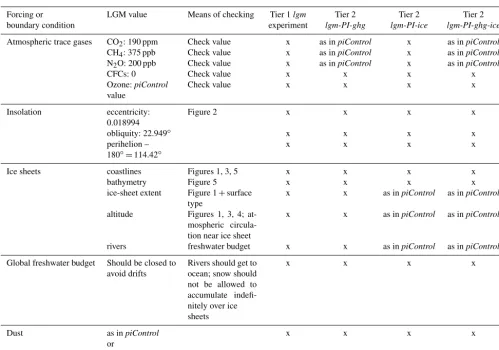
Figure 2. Top of the atmosphere difference in insolation (in W m−2) forlgm as compared to piControl (lgm– piControl), as a function of latitude and month of the year. There is no difference related to the calendar, which is the same for piControl andlgm, be-cause the difference between the definition of the modern calendar and the definition based on astronomy is not statistically significant for the LGM orbital configuration.
– obliquity=22.949◦,
– perihelion−180◦=114.42◦: the angle between the ver-nal equinox and the perihelion on the Earth’s trajectory should be set to 180+114.42◦, and
– the date of vernal equinox should be set to 21 March at noon.
The resulting insolation at the top of the atmosphere should then be similar to that displayed in Fig. 2, with a decrease at high latitudes during the summer hemisphere reaching over 10 W m−2and a mild increase (reaching 3 W m−2)between October and April at 40◦N, December and June at the Equa-tor, and mid-January to August at 40◦S.
4.3 Ice sheets
The ice sheet can be set to one of the following recon-structions (Fig. 1): GLAC-1D (Tarasov et al., 2012; Briggs et al., 2014; Ivanovic et al., 2016), ICE_6G-C (Peltier et al., 2015; Argus et al., 2014), or PMIP3 (Abe-Ouchi et al., 2015). GLAC-1D and ICE_6G-C are the most recent recon-structions and are compatible with the set-up of the PMIP4 deglaciation simulation (Ivanovic et al., 2016). The use of the PMIP3 ice-sheet reconstruction allows direct comparison with the PMIP3 simulations. These ice-sheet reconstructions significantly differ with each other, in particular in terms of altitude, with differences reaching several hundred metres over North America and Fennoscandia (Fig. 1 and Ivanovic et al., 2016, Fig. 2). This uncertainty in the boundary condi-tions results from the different approaches used for the recon-structions, which are summarized in Ivanovic et al. (2016).
LGM land fraction
sftlf
original file original resolution
LGM ice sheet fraction
sftgif
original file original resolution
Pre-industrial land fraction 1st computation of
LGM ocean boundaries & LGM surface types for the atmosphere
Check Ice sheets • North America • Northwestern
Europe • Antarctica/
Greenland
Check closure of • Bering Strait • Sunda & Sahul
Shelves • Connection
between Black and Mediterranean Seas
Check/include • Red Sea connection
to Arabian Sea • Connection of Sea
of Japan to Pacific • Caspian Sea
Final definition of LGM ocean boundaries & LGM surface types for the atmosphere
Weights for ocean-atmosphere coupling Final polishing of ocean boundaries according to model requirements
St
ep
0
St
ep
[image:9.612.48.293.64.247.2]1
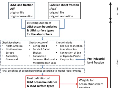
Figure 3.Summary of steps to be followed for the definition of the basic surface types for the atmosphere and ocean boundaries.
model (Fig. 3). The details of the implementation may dif-fer for other models, but the same steps should be followed and documented.
Step 0: Computing the land fraction (sftlf), land-ice fraction (sftgif), and orography (diff_orog) from the ice-sheet reconstruction data sets.
The PMIP3 reconstruction files include information about the land fraction (sftlf forsurfacetypelandfraction), land-ice fraction (sftgif forsurfacetypeglacierfraction), and dif-ference in orography (diff_orog) that needs to be applied to the piControl orography in order to obtain an lgm orogra-phy. This information, in particular sftlf, is not directly avail-able in the GLAC-1D reconstruction and is incomplete in the ICE-6G_C reconstruction (e.g. the Caspian Sea, above the present-day sea level, is missing). The variables available for each reconstruction are listed in Table 2. They can be found on the PMIP4 website (http://pmip4.lsce.ipsl.fr), as provided by the authors of the reconstructions. In particular, the vari-able names and the resolution have not been modified. In the present step 0, we describe how we compute sftlf, sftgif, and orog from the GLAC-1D and ICE-6G_C data. The IPSL model requires orog at 1/6◦ resolution for its gravity wave drag parameterization, which is why we compute diff_orog at this high resolution.
The procedure is as follows
(“Pre-pare_LGM_BC_files.py” Python script provided on the PMIP4 website):
– the input variables listed in Table 1 are read in; these in-clude the land fraction for ICE-6G_C but not for GLAC-1D;
– for GLAC-1D, the land–sea mask for the present and for the LGM are defined as where topography is positive;
– small holes (usually one to two isolated grid boxes) in the land-ice fraction are filled, using the “bi-nary_fill_holes” function of the python scipy/ndimage package (for ICE-6G_C, 155 points are filled in, to be compared to the total number of land-ice grid points, with is initially 423 610; for GLAC_1D, 62 points are filled in; the total number of points fully covered by land ice is 23 348);
– the land fraction is updated to include the land-ice frac-tion;
– this land fraction includes unrealistic isolated continen-tal points which are well below sea level (we have considered a threshold of−500 m. There are 23 such points in the ICE-6G_C case, 4 in the GLAC_1D case). These points are filled in using the same function as for the land-ice mask. However, several straits must be re-opened so that the function does not fill in the Red Sea, the Black Sea, the Azov Sea, the Sea of Japan, the Mediterranean Sea, and additionally the Per-sian Gulf, the Baltic and White seas, the Great Lakes, and the Canadian Archipelago for the present day. “bi-nary_fill_holes” is applied with the appropriate straits opened; then, these are closed again. sftlf is computed following this method for both the present and the LGM;
– the topography of the points that have been filled in is corrected by averaging the topography of the surround-ing points, after removsurround-ing points well below sea level; and
– the topography on the continents can be defined for the present and the LGM, and the difference in orogra-phy diff_orog can be computed. Similarly, differences in bathymetry can also be computed.
This preliminary step provides the three variables that are necessary to modify the boundary conditions for the atmo-sphere and the ocean: the land–sea mask, the land-ice mask, and the difference in topography and bathymetry. For the IPSL model, we keep the LGM orography computed at this step for further use.
Step 1. Defining the land–sea mask and the land-ice mask within the climate model
In the IPSL model, the coastlines are defined first for the ocean model and then they are used to compute the fraction of land and ocean on the atmospheric grid. We will there-fore follow this order here. The procedure is summarized in Fig. 3.
Table 2.Variables provided with the ice-sheet reconstructions considered for PMIP4.
GLAC-1D ICE-6G_C PMIP3
– HDC:
– on continents (including ice sheets) and ice shelves: surface altitude (in-cluding ice sheets/shelves)
– on ice-free ocean: bathymetry – HDCB:
– on continents (including ice sheets) and ice shelves: surface altitude (in-cluding ice sheets)
– on ice shelves: altitude of the bottom of the floating ice
– on ice-free ocean: bathymetry – ICEM: ice mask, fraction
– ice fraction values between 0.0 (no ice) and 1.0 (100 % ice)
– Topo: topography (point-value altitude, in metres)
– on continents: surface altitude (in-cluding grounded ice sheet)
– on ice-free oceans, and where there is floating ice (ice shelves): bathymetry
– Orog: orography (point-value surface altitude, in metres)
– on continents: altitude (including grounded ice sheet)
– on ice-free oceans: 0.0 (zero)
– on ice shelves: surface altitude – sftlf: point-value land mask, in %
– values are 0 (not land) or 100 (land)
– does not include floating ice – sftgif: point-value ice mask, in %
– values are 0 (not ice) or 100 (ice)
– floating ice is included
– diff_orog: LGM – present difference in orography
– sftlf: land fraction
– sftgif: grounded ice frac-tion
of land at locations of the main ice sheets, especially over areas that were glaciated at the LGM but that are covered by oceans today (such as Hudson Bay and the Barents–Kara seas); closure of the Bering Strait, of the straits between the Mediterranean and Black seas, and of the Sahul and Sunda shelves. At this stage, we re-introduce the Caspian Sea in the land–sea mask, using the present-day Caspian Sea. The Caspian Sea is absent from the land–sea masks computed from step 0 because it is higher than global sea level at the LGM. These basic coastlines need polishing, as a function of the ocean model, in order for ocean transport to occur in narrow straits. In particular, the connection from the Red Sea to the Arabian Sea should be checked, as well as of the Sea of Japan to the Pacific Ocean and narrow passages between the Sunda and Sahul shelves. This is detailed for the NEMO ocean in Program 2 given in the Supplement.
Once the ocean boundaries are set up, these can be interpo-lated over the atmospheric grid. The weights required to pass from one grid to the other are computed at the same time.
The land-ice cover is interpolated directly on the atmo-spheric grid and multiplied by the land–sea mask so that no land ice is defined over the ocean. This might differ for mod-els including a representation of ice shelves.
At the end of step 1, the coastlines are defined for the ocean model, and the land-ice and land–sea masks are de-fined for the atmospheric model.
Step 2. Implementing the LGM orography
The LGM orography is implemented by adding the LGM– present anomaly in orography computed in step 0 to the pi-Controlorography. This is straightforward for models that only require the average orography for each grid point. Additional steps are required for models requiring second-order moments/minimum/maximum values/slope character-istics for each grid point (e.g. the parameterization proposed by Lott and Miller, 1997). These moments must be com-puted from a high-resolution orography data set and the anomaly method should be applied for this high-resolution data set before computation of the parameters depending on fine-scale orography. The ice-sheet orography needs to be smoothed before this computation is made, to prevent un-realistic parameters due to the present-day orography (Fig. 4 illustrates the impacts of smoothing the topography for the north-western part of North America). These steps are de-tailed in program “Prepare_LGM_BC_files.py” (at step 6) given in the Supplement for the LMDZ model. The smooth-ing is performed with the Gaussian filter provided in the ndimage package, with sigma=3.
Step 3. Implementing the LGM bathymetry
Figure 4. (a, b)High-resolution orography obtained for north-western North America, by adding the ICE_6G-C orography anomaly on the piControl orography used for the LMDZ model.(c, d)The corresponding mean altitude over each grid point.(e, f)Standard deviation of the altitude within each grid point, to represent one of the parameters used in the gravity wave drag parameterizations. (a, c, e)Without smoothing on the ice sheets;(b, d, f)after smoothing on the ice sheets. The high-resolution ocean mask is plotted in white and the land-ice mask is outlined in black.
bathymetry used for the piControl simulations. However, given that the resolution of the ocean models often decreases with depth, this may not be necessary, and a simpler option is to modify the present-day bathymetry by subtracting the mean sea-level drop corresponding to the chosen ice-sheet reconstruction. In this second option, special treatment will be required for straits that are crucial for the ocean circula-tion and for which the change in bathymetry is significantly different from the mean sea-level drop. The Denmark and Davis straits and the Iceland–Faeroe Rise, for example, must be treated with care, as these are often locations at which the bathymetry for piControl is also adjusted to obtain re-alistic oceanic currents. The second option is used for the
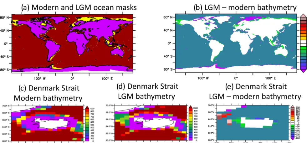
[image:11.612.127.468.64.469.2](a) Modern and LGM ocean masks
( b) LGM
–
modern bathymetry
( c) Denmark Strait
Modern bathymetry
( d) Denmark Strait
LGM bathymetry
[image:12.612.54.545.63.291.2]( e) Denmark Strait
LGM
–
modern bathymetry
Figure 5.Checking the bathymetry and coastlines (example of figures obtained with the ferret script verif_all.jnl provided in the Supple-ment).(a)Modern and LGM ocean masks (purple: continents in both modern and LGM configurations); yellow: continent in LGM config-uration, ocean in modern configuration; red: ocean in both modern and LGM configurations;(b)anomaly (LGM – modern) in bathymetry (m);(c, d, e)details for the Demark Strait/Iceland area;(c)modern bathymetry (m);(d)LGM bathymetry (m);(e)LGM – modern bathymetry anomaly (m).
area. We have ensured that the imposed change in bathymetry matches the reconstructed one for the Greenland–Iceland Rise and Iceland–Faeroe Rise.
4.4 Freshwater budget: rivers, runoff, and accounting for positive snow mass balance over the ice sheets The LGM sea-level drop leads to expanded continents and this can mean that prescribed river courses no longer reach the ocean. The North American and European ice sheets also disrupt river courses. At a minimum, the LGM rivers must be set up to ensure they reach the oceans. For instance, the European rivers that today drain into the Nordic and Baltic seas can be redirected to the North Atlantic via the paleo-English Channel (see e.g. Alkama et al., 2006). More real-istic river-routing files compatible with the ice-sheet recon-structions will also become available at a later stage.
It is highly possible that the snow mass balance over the ice sheets is positive, resulting in a sink of freshwater in the climate model. If this is the case, the average value of the sink (e.g. the average for a 10-year period) should be com-puted and released to an adjacent ocean, to guarantee closure of the freshwater budget. This should be done following the same procedures as for the DECK experiments or following the procedure advised since PMIP2, which was to compen-sate for the sink of freshwater by imposing a freshwater flux in broad regions of oceans adjacent to the ice sheets (e.g. the Arctic and North Atlantic north of 40◦N for the North Amer-ican ice sheet). As this decision might have a large impact on
the global ocean overturning circulation, it must be precisely documented (cf. Sect. 4.10).
4.5 Vegetation
4.6 Mineral dust
There are several options for implementing dust forcing ac-cording to the model’s complexity and to the availability of different data sets. Three series of dust data sets are pro-vided. Two of them are based on model simulations (Albani et al., 2014, 2016; Hopcroft et al., 2015). Both models in-clude a prognostic dust cycle, based on different formulations of the dependency of emissions on wind speed, soil moisture, and vegetation cover arising from the work of Marticorena and Bergametti (1995) and Fécan et al. (1999). In one case (Albani et al., 2014) pre-industrial vegetation is prescribed for physical climate for both PI and LGM climate condi-tions, but LGM dust emissions at each grid cell are scaled by the non-vegetated fraction, resulting from an offline vege-tation reconstruction with BIOME 4 (Kaplan et al., 2003), in equilibrium with LGM climate conditions. In the other case (Hopcroft et al., 2015) a dynamical vegetation model was used to determine the erodible surface. These differences re-sult in different dust emission fields. Furthermore, Albani et al. (2014, 2016) further refined their dust emissions by scal-ing the soil erodibility at the continental scale in order to have a better match to paleodust observations in terms of depo-sition fluxes. The third data set (Lambert et al., 2015) is a reconstruction of dust deposition, essentially based on geo-statistical interpolation of paleodust observations. The three data sets have different specifications in terms of dust size distribution: four size bins spanning 0.1–10 µm diameter (Al-bani et al., 2014), six size bins spanning 0.0316–31.6 µm ra-dius (Hopcroft et al., 2015), and bulk i.e. integrated over the entire observed size range (Lambert et al., 2015). This has implications for imposing proper constraints on the global dust cycle, e.g. magnitude of emissions (Albani et al., 2014), as well as for dust radiative forcing, when considered in com-bination with the prescribed dust optical properties (Kok et al., 2017). Therefore modelling groups should carefully ac-count for this aspect when integrating one of these data sets into their model framework.
For models with interactive dust modules but without dy-namic vegetation, it is advisable to take into account the more extensive dust sources at LGM. These are described by the “erodibility map” from the Albani et al. (2016) data set and a bare soil map for the Hopcroft et al. (2015) data (Fig. 6a and b, respectively). For these regions, vegetation must be set to either low vegetation (grasses) or bare soil; otherwise, the source functions should be adapted depending on the pre-cise formulation of the dust emission module in the particu-lar model (e.g. Ginoux et al., 2001) so that dust emissions are allowed. For models that compute the dust radiative forcing from atmospheric dust mass loading, two data sets are avail-able for the LGM: Albani et al. (2014, 2016) and Hopcroft et al. (2015). The prescribed LGM mass loading should be implemented as perturbations of the piControl loading, i.e. by either adding an anomaly to thesepiControlloads or by multiplying them by a ratio, the anomaly, or the ratio being
computed from the Albani et al. (2014, 2016) or Hopcroft et al. (2015) data sets. Alternatively, modelling groups can compute their own atmospheric dust mass loads offline and use them as prescribed fluxes in their coupled simulations.
Both dust data sets also provide radiative forcing. These should not be used directly because the specified radiative properties of dust vary among models, and using the forc-ing from the models used to produce the dust fields would be incompatible with other CMIP6 experiments. The dust ra-diative forcing provided with the data sets is only given with the purpose of broad comparison with the modelling groups’ own model output (Fig. 6c and d).
Models including marine biogeochemistry should use LGM dust deposition on the oceans, using the same data set as for the atmospheric forcing (Fig. 6e and f). If LGM dust atmospheric forcing cannot or is not taken into account, then the Lambert et al. (2015) data set can also be chosen (Fig. 6g).
Modelling groups undertaking the implementation of dust in their models are advised to perform a first trial with an atmosphere-only simulation, as run-away effects involving dust, vegetation, and climate have been experienced by some modelling groups (Hopcroft and Valdes, 2015b). In the latter case, it was the choice of parameters in the dynamic vegeta-tion model which proved to be inadequate.
4.7 Other inputs for ocean biogeochemistry models The global amount of dissolved inorganic carbon, alkalin-ity, and nutrients should be initially adjusted to account for the change in ocean volume. This can be done by multiply-ing their initial value by the relative change in global ocean volume. Other features that may need adjustment, given the changes in coastlines and bathymetry, include the amount of nutrients brought by rivers and by boundary exchange at the ocean–sediment interface. Modelling groups must document any such changes in the description of their simulations (cf. Sect. 4.10).
4.8 Initialization and spin-up
First, it is suggested to run the atmosphere model sepa-rately, using the sea surface temperatures and sea ice from the ocean’s initial conditions, in order for the atmosphere to adjust to the topography and surface-type changes. At this stage, it is advised to check that the total atmospheric mass (or globally averaged surface pressure) is the same as for piControl. This run will yield an initial state for the atmo-spheric component of the model.
Figure 6.Maps of active sources for dust emissions in the LGM and pre-industrial (PI) conditions in the simulations:(a)with the Community Earth System Model (Albani et al., 2014) and(b)with the Hadley Centre Global Environment Model 2-Atmosphere (Hopcroft et al., 2015). Maps of LGM dust aerosol optical depth (AOD) from the simulations of(c)Albani et al. (2014) and(d)Hopcroft et al. (2015). Maps of LGM dust deposition (g m−2a−1)(e)simulated with the Community Earth System Model (Albani et al., 2014),(f)simulated with the Hadley Centre Global Environment Model 2-Atmosphere (Hopcroft et al., 2015), and(g)reconstructed from a global interpolation of paleodust data (Lambert et al., 2015).
Standard Mean Ocean Water (SMOW) of+1 ‰. The ocean model can be initialized from apiControlexperiment or from previous LGM experiments, to minimize spin-up duration.
Practically, the ocean model can be generally initialized from apiControlocean state with adjusted salinity (and oxy-gen isotope, if applicable), or from previous LGM experi-ments (e.g. with well-stratified glacial ocean states), to min-imize spin-up duration. Such ocean states, such as described in Werner et al. (2016), which provide 3-D fields of sea tem-perature, salinity, and associated stable water isotopes on a regular 1◦×1◦grid, are available on the PMIP4 website and from the PMIP2 and PMIP3 databases.
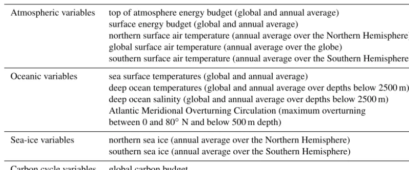
The model should be spun up until equilibrium. In pre-vious PMIP protocols (in particular http://pmip2.lsce.ipsl.fr) the simulations were considered at equilibrium when the trend in globally averaged SST was less than 0.05◦C/century, the Atlantic Meridional Overturning Circulation (AMOC) was stable and, for models including representations of the carbon cycle or dynamic vegetation, the requirement was that the carbon uptake or release by the biosphere is less than 0.01 Pg C per annum. Recent works give other criteria or rec-ommendations for defining or reaching the equilibrium. For instance, to avoid impacts of potential transient
character-istics in the deep ocean on AMOC strength (Zhang et al., 2013), the equilibrium ocean should ensure that the trend in zonal mean sea salinity in the Southern Ocean (south of the winter sea-ice edge) remains small, especially in the Atlantic sector. Marzocchi and Jansen (2017) show that the AMOC has to be monitored on multi-centennial timescales because variability on the timescales of decades to a century prevents a precise determination of the trends, and hence of whether the model is close to equilibrium or not.
Table 3.Variables to be saved for the documentation of the spin-up phase of the models.
Atmospheric variables top of atmosphere energy budget (global and annual average) surface energy budget (global and annual average)
northern surface air temperature (annual average over the Northern Hemisphere) global surface air temperature (annual average over the globe)
southern surface air temperature (annual average over the Southern Hemisphere)
Oceanic variables sea surface temperatures (global and annual average)
deep ocean temperatures (global and annual average over depths below 2500 m) deep ocean salinity (global and annual average over depths below 2500 m) Atlantic Meridional Overturning Circulation (maximum overturning between 0 and 80◦N and below 500 m depth)
Sea-ice variables northern sea ice (annual average over the Northern Hemisphere) southern sea ice (annual average over the Southern Hemisphere)
Carbon cycle variables global carbon budget
4.9 Potential problems
Experience gained from previous phases of PMIP suggests there can be several problems setting up an LGM simulation, including
– failure to close the freshwater budget, which can arise from either inadequate compensation for a positive snow mass balance over the ice sheets or from rivers not reaching the ocean,
– numerical instabilities in the atmosphere, especially near or above the ice sheets, and
– run-away cooling due to climate–vegetation–dust feed-backs, as reported by Hopcroft and Valdes (2015b). In this case the dynamic vegetation scheme was found to be overly sensitive to temperature, so that grass plant functional types started to die back below 5◦C, resulting in higher albedo, further cooling, and eventual desertifi-cation across most of Eurasia in the first LGM simula-tion with HadGEM2-ES.
4.10 Documenting the simulations
The documentation of the simulations should include – the model version used, in particular in terms of
vegeta-tion and dust representavegeta-tions (interactive, prescribed, or absent),
– the ice-sheet reconstruction chosen and how it has been implemented,
– how river routing has been modified and how positive snow mass balance over the ice sheets is dealt with, in particular the regions over which the excess freshwater is applied,
– the vegetation used in the simulation and how it was obtained and/or implemented,
– the dust reconstruction used and how it has been imple-mented,
– the forcings used (dust, nutrients from rivers and sed-iments) if ocean biogeochemistry is included in the model, and
– the spin-up strategy and duration, with documentation of the variables listed in Table 3.
A PMIP4 special issue in GMD and Climate of the Past is open so that groups can publish these documentations. Mod-elling groups are also encouraged to contribute their simula-tion and model documentasimula-tion to the ES-DOC facility. 4.11 “ripf”code for the simulations
CMIP6 simulations can be documented through their “ripf” code, these letters standing for “realization”, ‘initialization”, “physics”, and “forcing”. In practice, each of these letters is followed by a number which indicates
– after the “r”: the simulation number in the ensemble of simulations with the same characteristics;
– after the “i”: the initial method;
– after the “p”: the chosen model’s physics; and – after the “f”: the forcing used for the simulation. Since there are multiple choices for setting up PMIP4-CMIP6 and PMIP4 LGM experiments, we propose the sys-tematic use of common “f” indices within the CMIP6 “ripf” indices so that the simulations can be distinguished easily from each other.
The first digit should describe the ice-sheet reconstruction. It should be set to
– for GLAC-1D, and – for PMIP3.
The second digit should describe the vegetation. It should be set to
– 0 ifpiControlvegetation is used,
– 1 if an LGM vegetation is prescribed, and
– 2 if the model includes a dynamical vegetation model. The third and fourth digits should describe how dust is in-cluded in the set-up.
– If no dust forcing can be taken into account, they should be set to 00.
– If dust is prescribed from a PMIP4 data set, they should be set to
– 11 for the Albani et al. (2014, 2016) data set, – 12 for the Hopcroft et al. (2015) data set,
– 13 for the Lambert et al. (2015) data set (for ocean biogeochemistry models only), and
– 19 for the modelling group’s own dust forcing. – If dust is interactively computed, they should be set to
– 20 if the surface maps are dynamically simulated using a coupled dynamic vegetation scheme, – 21 if the surface maps for emissions are those from
Albani et al. (2014, 2016),
– 22 if the surface maps for emissions are those from Hopcroft et al. (2015), and
– 29 if the surface maps for emissions are produced by the modelling group itself, e.g. by using an of-fline vegetation model.
4.12 Output
The data should be formatted so as to comply with the CMIP6 standards (to be documented in the GMD CMIP6 special issue; cf. Eyring et al., 2016) and PMIP4 data re-quest (Kageyama et al., 2016) so that analyses including other PMIP and CMIP6 simulations can be performed easily. The current list of variables is given in the Supplement but is still subject to potential changes following adjustments of the full CMIP6 list. The PMIP4 data request can be found on the PMIP4 website (https://pmip4.lsce.ipsl.fr/doku.php/ database:pmip4request#the_pmip4_request).
5 Analyses and outlook
The LGM experiment is a major investment by climate mod-elling groups, but provides a demanding test of model reli-ability under extreme and well-documented conditions. In-deed, our experience is that several groups have found model errors while setting up their LGM climate simulations, in par-ticular in the coupling between the atmosphere and the ocean and in the global freshwater budget. The PMIP4-CMIP6 sim-ulations, along with PMIP4 sensitivity experiments and pre-vious PMIP2 and PMIP3 experiments, will create an un-precedented data set about the LGM climate state. With a larger number of simulations, and a better sampling of the forcing uncertainties, we should be able to reach more robust conclusions about, for example,
– the ability of state-of-the-art climate models to repre-sent a climate very different from the pre-industrial or present climates: benchmarking these simulations will provide a measure of how well models simulate large climate changes, comparable in magnitude to changes expected over the 21st century. Although there are data sets documenting environmental conditions and climate at the LGM, the planned PMIP4-CMIP6 analyses would benefit from the improvement and geographic expan-sion of these data sets. In addition, there is scope for the creation of new data sets, particularly data sets that can be used to evaluate aspects of the more complex Earth system models that are being run in PMIP4-CMIP6; – the relationships between climate or environmental
changes at far away locations, or between different fea-tures of the climate system: for instance, as alluded to in the introduction, we expect the atmospheric and ocean circulations in the North Atlantic area to be sen-sitive to the ice-sheet height; the PMIP4-CMIP6 exper-imental design allows for multi-model studies on this topic; at large scales, the polar amplification and land– sea contrasts that have been studied with PMIP2 and PMIP3 experiments could be altered with the PMIP4 more complex simulations including vegetation or/and dust changes; and
– the potential constraint from the LGM (in particular via the LGM tropical SSTs) on climate sensitivity.
The Tier 2 sensitivity experiments will allow the quantifi-cation of the role of individual forcings and feedbacks in mate. This is an essential step in understanding the LGM cli-mate, but also in characterizing and understanding common and/or contrasting features of the most recent past warming (between the LGM and the present) and the predicted future warming.
other CMIP6 projects and we hope these data will also be analysed by experts from other CMIP6 MIPs. For instance, the understanding of the impacts of the LGM climate forc-ings and the role of radiative feedbacks is related to CFMIP (Webb et al., 2017) and RFMIP (Pincus et al., 2016). The PMIP4 single forcing experiments can be used in view of the CFMIP experiments testing the impact of uniform low-ering of SSTs or CO2decrease (in AMIP configuration) and the connection to climate sensitivity for CO2increase should be made easier to analyse with these experiments. In terms of diagnostics that can be used to analyse the role of each component of the climate models in setting up the LGM cli-mate, we also expect new studies based on diagnostics devel-oped by the CMIP6 MIPs on the ocean (OMIP, Griffies et al., 2016; Orr et al., 2017), land surface and snow (LS3MIP, van den Hurk et al., 2016), aerosols (AerChemMIP, Collins et al., 2017), sea ice (SIMIP, Notz et al., 2016), and ice sheets (IS-MIP6, Nowicki et al., 2016). It is therefore important to keep the relevant output for these analyses, and the PMIP4 data request has been built based on the lists for these other MIPs. LGM experiments will also be the starting point for sim-ulations of the last deglaciation, i.e. the transition from the full glacial state to the present interglacial state (21–9 ky BP) and through to the present (Ivanovic et al., 2016). Given the large and abrupt changes in AMOC during the glacial pe-riod and during the deglaciation, the LGM will also be a reference state for freshwater hosing studies, which will al-low further analyses of the relationships between the AMOC state and climate. This is relevant for studying the processes at work during Heinrich events 1 and 2, but also for estab-lishing a coherent view of the LGM physical climate sys-tem state throughout all its components. Stated in a differ-ent manner, analysinglgmsimulations characterized by dif-ferent AMOCs, obtained through freshwater hosing or not, will help to determine whether all the reconstructions that are available for the different components of the climate sys-tem (state of the AMOC, state of the ocean surface, state of the continental surface) are consistent from the point of view of the physics summarized in a climate model, as suggested by studies carried out with one model (Zhang et al., 2013; Klockmann et al., 2016).
This brief outline of possible analyses of the PMIP4-CMIP6 lgm simulations is not meant to be exhaustive, but rather to illustrate how these simulations will contribute to progress on the overarching questions of CMIP6.
Code and data availability. All the forcing data sets, their refer-ences, and their code can be found on the PMIP4 website (https: //pmip4.lsce.ipsl.fr/doku.php/exp_design:lgm, PMIP4 repository, 2017). The forcings will also be added to the ESGF Input4MIPS repository (https://esgf-node.llnl.gov/projects/input4mips/, with de-tails provided in the “input4MIPs summary” link).
Acknowledging CMIP6 according to the instructions given in Eyring et al. (2016), PAGES, and WCRP, which endorse PMIP, as
well as the modelling groups which have contributed to the CMIP6 and PMIP4 effort, will be greatly appreciated.
The Supplement related to this article is available online at https://doi.org/10.5194/gmd-10-4035-2017-supplement.
Competing interests. The authors declare that they have no conflict of interest.
Acknowledgements. Masa Kageyama and Qiong Zhang
acknowl-edge funding from French–Swedish project GIWA. Sandy P. Harrison acknowledges funding from the European Research Council for “GC2.0: Unlocking the past for a clearer future”. Ruza F. Ivanovic is funded by a NERC Independent Research Fellowship (no. NE/K008536/1). Fabrice Lambert acknowledges support from CONICYT projects 15110009, 1151427, ACT1410, and NC120066. Bette L. Otto-Bliesner, Esther C. Brady, and Robert A. Tomas acknowledge the funding by the U.S. National Science Foundation of the National Center for Atmospheric Research. Peter O. Hopcroft is funded by UK NERC (NE/I010912/1 and NE/P002536/1).
Edited by: James Annan
Reviewed by: two anonymous referees
References
Abe-Ouchi, A., Saito, F., Kageyama, M., Braconnot, P., Harrison, S. P., Lambeck, K., Otto-Bliesner, B. L., Peltier, W. R., Tarasov, L., Peterschmitt, J.-Y., and Takahashi, K.: Ice-sheet configuration in the CMIP5/PMIP3 Last Glacial Maximum experiments, Geosci. Model Dev., 8, 3621–3637, https://doi.org/10.5194/gmd-8-3621-2015, 2015.
Albani, S., Mahowald, N. M., Perry, A. T., Scanza, R. A., Zen-der, C. S., Heavens, N. G., Maggi, V., Kok, J. F., and Otto-Bliesner, B. L.: Improved dust representation in the Commu-nity Atmosphere Model, J. Adv. Model. Earth Syst., 6, 541–570, https://doi.org/10.1002/2013MS000279, 2014.
Albani, S., Mahowald, N. M., Murphy, L. N., Raiswell, R., Moore, J. K., Anderson, R. F., McGee, D., Bradtmiller, L. I., Del-monte, B., Hesse, P. P., and Mayewski, P. A.: Paleodust vari-ability since the Last Glacial Maximum and implications for iron inputs to the ocean, Geophys. Res. Lett., 43, 3944–3954, https://doi.org/10.1002/2016GL067911, 2016.
Alkama, R., Kageyama, M., and Ramstein, G.: Freshwater dis-charges in a simulation of the Last Glacial Maximum climate using improved river routing, Geophys. Res. Lett., 33, L21709, https://doi.org/10.1029/2006GL027746, 2006.
Annan, J. D. and Hargreaves, J. C.: A perspective on model-data surface temperature comparison at the Last Glacial Maximum, Quaternary Sci. Rev., 107, 1–10, 2015.
(VM5a) based on GPS positioning, exposure age dating of ice thicknesses, and relative sea level histories, Geophys. J. Int., 198, 537–563, https://doi.org/10.1093/gji/ggu140, 2014.
Bartlein, P. J., Harrison, S. P., Brewer, S., Connor, S., Davis, B. A. S., Gajewski, K., Guiot, J., Harrison-Prentice, T. I., Hender-son, A., Peyron, O., Prentice, I. C., Scholze, M., Seppä, H., Shu-man, B., Sugita, S., Thompson, R. S., Viau, A., Williams, J., and Wu, H.: Pollen-based continental climate reconstructions at 6 and 21 ka: a global synthesis, Clim. Dynam., 37, 775–802, 2011. Beghin, P., Charbit, S., Kageyama, M., Combourieu Nebout, N.,
Hatté, C., Dumas, C., and Peterschmitt, J.-Y.: What drives LGM precipitation over the western Mediterranean? A study focused on the Iberian Peninsula and northern Morocco, Clim. Dynam., 46, 2611–2631, 2016.
Bereiter, B., Eggleston, S., Schmitt, J., Nehrbass-Ahles, C., Stocker, T. F., Fischer, H., Kipfstuhl, S., and Chappellaz, J.: Revision of the EPICA Dome C CO2 record from 800 to 600 kyr before present, Geophys. Res. Lett., 42, 542–549, https://doi.org/10.1002/2014GL061957, 2015.
Berger, A.: Long-term variations of daily insolation and quaternary climatic changes, J. Atmos. Sci., 35, 2362–2367, 1978. Böhm, E., Lippold, J., Gutjahr, M., Frank, M., Blaser, P., Antz,
B., Fohlmeister, J., Frank, N., Andersen, M. B., and Deininger, M.: Strong and deep Atlantic meridional overturning cir-culation during the last glacial cycle, Nature, 517, 73–76, https://doi.org/10.1038/nature14059, 2015.
Bopp, L., Kohfeld, K. E., Le Quéré, C., and Aumont, O.: Dust impact on marine biota and atmospheric CO2 during glacial periods, Paleoceanography, 18, 1046, https://doi.org/10.1029/2002PA000810, 2003.
Boucher, O., Randall, D., Artaxo, P., Bretherton, C., Feingold, G., Forster, P., Kerminen, V.-M., Kondo, Y., Liao, H., Lohmann, U., Rasch, P., Satheesh, S. K., Sherwood, S., Stevens, B., and Zhang, X. Y.: Clouds and Aerosols, in: Climate Change 2013: The Phys-ical Science Basis. Contribution of Working Group I to the Fifth Assessment Report of the Intergovernmental Panel on Climate Change, edited by: Stocker, T. F., Qin, D., Plattner, G.-K., Tig-nor, M., Allen, S. K., Boschung, J., Nauels, A., Xia, Y., Bex, V., and Midgley, P. M., Cambridge University Press, Cambridge, UK and New York, NY, USA, 2013.
Braconnot, P. and Kageyama, M.: Shortwave forcing and feedbacks in Last Glacial Maximum and Mid-Holocene PMIP3 simulations, Phil. Trans. R. Soc. A, 373, 20140424, https://doi.org/10.1098/rsta.2014.0424, 2015.
Braconnot, P., Otto-Bliesner, B., Harrison, S., Joussaume, S., Pe-terchmitt, J.-Y., Abe-Ouchi, A., Crucifix, M., Driesschaert, E., Fichefet, Th., Hewitt, C. D., Kageyama, M., Kitoh, A., Laîné, A., Loutre, M.-F., Marti, O., Merkel, U., Ramstein, G., Valdes, P., Weber, S. L., Yu, Y., and Zhao, Y.: Results of PMIP2 coupled simulations of the Mid-Holocene and Last Glacial Maximum – Part 1: experiments and large-scale features, Clim. Past, 3, 261– 277, https://doi.org/10.5194/cp-3-261-2007, 2007.
Braconnot, P., Harrison, S. P., Kageyama, M., Bartlein, P. J., Masson-Delmotte, V., Abe-Ouchi, A., Otto-Bliesner, B., and Zhao, Y.: Evaluation of climate models using palaeoclimatic data, Nature Climate Change, 2, 417–424, 2012.
Brady, E. C., Otto-Bliesner, B. L., Kay, J. E., and Rosenbloom, N.: Sensitivity to glacial forcing in CCSM4, J. Climate, 26, 1901– 1925, 2013.
Briggs, R. D., Pollard, D., and Tarasov, L.: A data-constrained large ensemble analysis of Antarctic evo-lution since the Eemian, Quat. Sci. Rev., 103, 91–115, https://doi.org/10.1016/j.quascirev.2014.09.003, 2014.
Claquin, T., Roelandt, C., Kohfeld, K. E., Harrison, S. P., Prentice, I. C., Balkanski, Y., Bergametti, G., Hansson, M., Mahowald, N., Rodhe, H., and Schulz, M.: Radiative forc-ing effect of ice-age dust, Clim. Dynam., 20, 193–202, https://doi.org/10.1007/s00382-002-0269-1, 2003.
CLIMAP project members: Seasonal reconstructions of the earth’s surface at the Last Glacial Maximum, Map Chart Series MC-36, Geological Society of America, Boulder, Colorado, 1981. Collins, W. J., Lamarque, J.-F., Schulz, M., Boucher, O., Eyring, V.,
Hegglin, M. I., Maycock, A., Myhre, G., Prather, M., Shindell, D., and Smith, S. J.: AerChemMIP: quantifying the effects of chemistry and aerosols in CMIP6, Geosci. Model Dev., 10, 585– 607, https://doi.org/10.5194/gmd-10-585-2017, 2017.
Crucifix, M.: Does the Last Glacial Maximum constrain climate sensitivity?, Geophys. Res. Lett., 33, L18701, https://doi.org/10.1029/2006GL027137, 2006.
Eyring, V., Bony, S., Meehl, G. A., Senior, C. A., Stevens, B., Stouffer, R. J., and Taylor, K. E.: Overview of the Coupled Model Intercomparison Project Phase 6 (CMIP6) experimen-tal design and organization, Geosci. Model Dev., 9, 1937–1958, https://doi.org/10.5194/gmd-9-1937-2016, 2016.
Fécan, F., Marticorena, B., and Bergametti, G.: Parametrization of the increase of the aeolian erosion threshold wind friction veloc-ity due to soil moisture for arid and semi-arid areas, Ann. Geo-phys., 17, 149–157, https://doi.org/10.1007/s00585-999-0149-7, 1999.
Ginoux, P., Chin, M., Tegen, I., Prospero, J., Holben, B., Dubovik, O., and Lin, S.-J.: Sources and distributions of dust aerosols sim-ulated with the GOCART model, J. Geophys. Res., 106, 20255– 20273, 2001.
Griffies, S. M., Danabasoglu, G., Durack, P. J., Adcroft, A. J., Bal-aji, V., Böning, C. W., Chassignet, E. P., Curchitser, E., Deshayes, J., Drange, H., Fox-Kemper, B., Gleckler, P. J., Gregory, J. M., Haak, H., Hallberg, R. W., Heimbach, P., Hewitt, H. T., Hol-land, D. M., Ilyina, T., Jungclaus, J. H., Komuro, Y., Krasting, J. P., Large, W. G., Marsland, S. J., Masina, S., McDougall, T. J., Nurser, A. J. G., Orr, J. C., Pirani, A., Qiao, F., Stouffer, R. J., Taylor, K. E., Treguier, A. M., Tsujino, H., Uotila, P., Valdivieso, M., Wang, Q., Winton, M., and Yeager, S. G.: OMIP contribution to CMIP6: experimental and diagnostic protocol for the physical component of the Ocean Model Intercomparison Project, Geosci. Model Dev., 9, 3231–3296, https://doi.org/10.5194/gmd-9-3231-2016, 2016.
Hargreaves, J. C., Annan, J. D., Yoshimori, M., and Abe-Ouchi, A.: Can the Last Glacial Maximum constrain climate sensitivity?, Geophys. Res. Lett., 39, L24702, https://doi.org/10.1029/2012GL053872, 2012.
Harrison, S. P., Bartlein, P. J., Brewer, S., Prentice, I. C., Boyd, M., Hessler, I., Holmgren, K., Izumi, K., and Willis, K.: Climate model benchmarking with glacial and mid-Holocene climates, Clim. Dynam., 43, 671–688, 2014.