A Gene Network Model for Developing Cell
Lineages
Nicholas Geard
1∗and Janet Wiles
1,21
School of Information Technology and Electrical Engineering
2
School of Psychology
The University of Queensland,
St Lucia, Queensland 4072, Australia
Telephone: +61 7 3365 1636
{
nic, j.wiles
}
@itee.uq.edu.au
Abstract
Biological development is a remarkably complex process. A single cell, in an appropriate environment, contains sufficient information to generate
a variety of differentiated cell types, whose spatial and temporal dynamics interact to form detailed morphological patterns. While several different physical and chemical processes play an important role in the development of an organism, the locus of control is the cell’s gene regulatory network.
We designed dynamic recurrent gene network (DRGN) model and eval-uated its ability to control the developmental trajectories of cells during embryogenesis. Three tasks were developed to evaluate the model,
in-spired by cell lineage specification inC. elegans, describing the variation
in gene activity required for early cell diversification, combinatorial
con-trol of cell lineages and cell lineage termination. Three corresponding sets of simulations compared performance on the tasks for different gene net-work sizes, demonstrating the ability of DRGNs to perform the tasks with minimal external input. The model and task definition represent a new
means of linking the fundamental properties of genetic networks with the topology of the cell lineages whose development they control.
Keywords: gene regulation, cell lineage, development, recurrent
1
Introduction
The development of a single, fertilised egg cell into a multicellular organism
is one of the most complex processes in biology [38]. Each cell in a growing
embryo contains an identical set of instructions encoded in its genome, yet it
follows a unique developmental trajectory that specifies both the type of cell
into which it will differentiate, as well as its location in the embryo. One major
area of investigation within developmental biology is how the developmental
trajectories of cells are programmed by a distributed network of interacting
genes [7].
The field of artificial life has made extensive use of the concept of
develop-ment, which it recognises as a powerful and highly evolvable means of encoding
design solutions [3]. While this view has led many researchers in artificial life
to approach biology as a source of novel ideas capable of revolutionising
engi-neering and other domains [32], artificial life also has the potential to make a
contribution to theoretical biology [9]. Two requirements render this a
challeng-ing task; suitable computational models must be chosen to represent biological
systems, and these models must be communicated in a fashion that is accessible
to a wider scientific audience.
A requirement for modelling any complex system is to determine an
ap-propriate level of abstraction, at which the properties that the model seeks to
investigate will emerge from interactions between well-understood agents at a
lower level of description. The goal when developing models of biological systems
is to balance simplicity with plausibility. If a model is too simplistic, extensions
to biology may be unconvincing, and findings will lack cogency. Conversely,
overly elaborate models that include unnecessary details will obscure the
essen-tial dynamics of the process under investigation. Furthermore, to communicate
to a biological audience, the computational tasks in a simulation study need to
Development is an interesting computational challenge because the
informa-tion required to specify each of a potentially large number of cell lineages is
contained in the regulatory interactions of a single network of genes. A variety
of genetic regulatory network (GRN) models have been developed to simulate
aspects of biological development, including the effect of interplay between
mul-tiple interacting mechanisms [12, 16], the role played by physical interactions [10]
and the dynamics of intercellular communication [13]. One issue that has not
been explicitly addressed is the relationship between the regulatory complexity
of a GRN and its ability to autonomously specify the developmental trajectories
of a group of cells.
In this study, we developed a dynamic recurrent gene network (DRGN1)
model, capable of generating developmental cell lineages. Our hypothesis is
that this model, despite its simplicity, possesses a sufficiently flexible range of
dynamic behaviours to enable it to generate complex developmental
trajecto-ries. Specifically, this study considers the situation in which a GRN receives
only limited external input and so is almost exclusively reliant on its internal
regulatory interactions to store a developmental program.
The next section of this paper reviews the biological background of our
study, briefly describing the process of development and the role that gene
regulation plays in determining a cell’s fate. Previous computational approaches
to modelling gene regulation and development are then reviewed before the
DRGN model is introduced. Several tasks are used to explore the capabilities of
the model, including the initial diversification of cells, the generation of specific
patterns of differentiation and the control of cell lineage termination. Finally,
the performance of the model and potential implications of the results discussed.
2
Development and Cell Lineage
The development of an embryo involves a variety of interacting processes,
in-cluding the growth, division and differentiation of cells and the specification
of body plans. Although the formation of physical structure in a developing
embryo involves mechanical factors such growth, cell migration and differential
adhesion, the information that determines whether the end product will be a
worm or a whale is encoded in the genome [7]. This section describes the process
of cell differentiation and the role that gene regulation plays in specifying cell
lineages.
2.1
Cell Differentiation
Cell differentiation is the process by which cells undergo physical and chemical
changes that result in them becoming structurally and functionally distinct.
From an initial egg cell, each successive cell division results in a new generation
of cells whose final fate is more determined. Upon reaching its terminal, fully
differentiated state, each cell will function as, for example, a nerve, muscle or
blood cell.
The primary feature that determines the function of a fully differentiated
cell is the proteins it contains [1]. Similarly, the most important property
char-acterising a developing cell is its pattern of gene activity [38]. Externally, the
cells of an early embryo may be virtually indistinguishable. Already, however,
the differences in their patterns of gene activity determine the role they and
their progeny will play in the fully developed organism. When a cell divides,
this pattern of active and inactive genes is passed on to its daughter cells via
positive regulatory feedback, and physical and chemical modifications to the
genome [38].
Patterns of gene activity are dynamic, changing over time as cells become
dynamics and a response to signals from the extracellular environment. The
sequence of changes in gene expression that a cell exhibits on its way to becoming
differentiated forms the developmental history, or lineage, of that particular cell.
An organism’s cell lineage is the sum of the lineages of its individual cells. Cell
lineages form a binary tree structure, where the root node represents an initial
egg cell, a branch point represents a division event and the leaf nodes represent
a set of terminally differentiated cells. An important question in developmental
biology is how the sequence of differentiation events is controlled to produce
complex patterns of terminal cells.
2.2
The Control of Cell Lineages by Gene Regulation
In a eukaryotic cell, the genetic regulatory system is encoded in the genome,
which is located in the cell’s nucleus. As well as carrying out various functions
related to cell maintenance and function, a significant portion of the genetic
system is involved in programming embryonic development [38].
The process of gene expression begins when an RNA polymerase molecule
binds to the start site of a gene, unwinds a section of DNA and uses one of the
strands as a template to transcribe messenger RNA (mRNA) molecules. mRNA
molecules are transported outside of the cell nucleus to the cytoplasm, where
they are translated into proteins. Proteins can either be structural, enabling a
cell to fulfil its functional role in an organism, or they can re-enter the nucleus
to regulate the expression of other genes. These regulatory proteins, known
as transcription factors (TFs), interact with the promoter and control regions
of a gene to either enhance or inhibit the transcription of that gene. Some
TFs are required for any transcription to occur at all. Others play a role as
activators, binding to enhancer sites located upstream or downstream of the
gene to facilitate transcription. Yet another type acts as a repressor, either by
gene start site [1].
When a cell divides, the set of TFs that determine its pattern of gene
ac-tivation are divided between the daughter cells, so each will generally have a
similar pattern of gene expression to its parent. On occasion, the distribution
of TFs in the parent cell may be asymmetric [19]. The two daughter cells will
therefore inherit different sets of regulatory information and hence follow two
unique developmental trajectories.
Inductive signals originating from other cells or the environment can also
alter patterns of gene expression. In general, these signalling molecules bind to
receptors found on the cell surface, and the signal is transmitted to the nucleus
via a series of chemical events called a signal transduction pathway. The role of
these signals is selective, they choose one fate from among the relatively small
number of possible trajectories defined by the current state of the cell [38].
For this study, the selection of an appropriate level of detail from the myriad
of facts known about biological development required focusing on two essential
aspects of gene regulation. Firstly, genes may be grouped into two classes,
regulatory genes that control the expression of other genes (including other
reg-ulatory genes) and structural genes that specify the functional roles of different
types of cells. Secondly, when a cell divides, both daughter cells inherit the
genetic network of the parent cell, including the structure of the regulatory
in-teractions and their level of activity. However, they also receive information that
differentiates between them, either through asymmetric division of determinants
or inductive signals from other cells.
2.3
The Embryonic Development of
C. elegans
Designing appropriate tasks to test a model of development requires explicitly
defining the genetic information inherent in control decisions. Gene expression
mi-croarray data represents an average across a population of cells and therefore
lacks the specificity of individual cell trajectories. Analysis of the phenotypic
effects resulting from mutations to particular genes is another potential source
of patterns, however, comprehensive data has been obtained for only a subset
of the relevant genes [29]. Our approach therefore has been to examine the cell
lineages themselves, with the aim of modelling the control decisions guiding
dif-ferentiation as represented by the topology of the cell lineage and the identities
of the terminal cells [6].
In most multicellular organisms, cell lineages follow a general plan for a
given species, with a certain amount of variation in the trajectories of individual
cells. Some species are remarkably resilient to environmental factors, with well
established developmental trajectories. Others, such as many plant species, are
very responsive to their environmental conditions. In this study, in order to
target the control decisions for differentiation as closely as possible to a known
biological system, we based the simulation tasks on the embryonic development
ofCaenorhabditis elegans (C. elegans), an organism with an exceptionally well
characterised cell lineage.
C. elegansis a small (approximately 1mm as an adult) worm found
through-out the world. It has become an important model organism for developmental
biologists for several reasons, some of which also make it an attractive subject
for computational modelling. Most notably, it has a relatively small number
of cells (959, plus a variable number of germ cells, as a developed adult) and
an invariant cell lineage, making it possible to gather a considerable amount of
data on its developmental processes. Despite its relative simplicity however, it
shares many genetic mechanisms with other species, including humans [38].
The first complete observation ofC. elegans embryogenesis was carried out
in 1983 [36], resulting in a diagram of the entire cell lineage. Since then, there
has been a gradual growth in understanding the way that gene expression and
mechanisms have been uncovered, the full picture is still incomplete [24].
A significant advance in understanding C. elegans development occurred
when new experimental techniques allowed the observation, not only of cell
lineage, but also of cell position throughout embryogenesis [31]. Based on these
observations, the three-dimensional structure of the initial stages ofC. elegans
embryogenesis was modelled computationally by Kitano and colleagues [22].
Their primary focus was on visualising cell position data, however, and only
limited connections were made to the underlying dynamics of gene expression.
By contrast, our model does not explicitly represent the physical structure of
the embryo, but focuses on the sequence of control decisions underlying the
developmental process, from which cell identity and embryonic structure emerge.
3
Modelling Gene Regulation and Development
Recent years have seen a rapid growth in the use of modelling as a tool to develop
intuitions about biological processes, providing insights into natural
computa-tion for both artificial and real life researchers. Approaches to modelling gene
networks range from detailed, mathematical models tied closely to experimental
data (see [8, 15] for recent reviews) to more abstract models from the fields of
complex systems and artificial life (e.g. [21, 34]). While the former is often used
to make quantitative predictions and generate empirically testable hypotheses,
the latter aims to develop insights about high-level properties of gene regulation.
The DRGN model follows the latter approach. It was inspired by biology,
and aims to generate insights that can inform our understanding of biology.
However, we use a level of description that attempts to capture the general
principles of biological development while abstracting away from as much
3.1
Boolean and Continuous Models of Gene Regulation
As described in Section 2.2, gene expression is regulated by interactions between
the multiple transcription factors that bind to a gene’s control region. Because
many of these factors are the products of other gene transcription events, they
too are under regulatory control. A genetic system can therefore be described in
terms of a network in which nodes represent genes and links represent regulatory
interactions. The state of a system at any given time can be described by the
levels of activation of all the genes in the system. The activation of any given
gene can be defined as a function of the current state of the system and any
environmental inputs. Thus future states of the system can be predicted from
the current pattern of gene expression.
Several different approaches have been applied to modelling gene regulation.
In the simplest case, genes are represented as nodes that are either on or off
(i.e. either expressed or not) and the condition for activation of a node is
repre-sented as a Boolean function of its input [21]. Depending on size, connectivity
and the choice of node activation functions, such systems are capable of
dis-playing a variety of dynamic behaviours, ranging from ordered fixed-point and
cyclic attractors to disordered or “chaotic” dynamics [21, 39]. As well as being
subjected to considerable theoretical investigation, Boolean networks have also
been used to model specific biological processes such as the cell cycle [18] and
pattern formation [4]. Other GRN models have used networks in which nodes
have continuous, rather than Boolean, levels of activation [27, 33, 37]. Genes
in biological systems display a continuous range of activity levels and it has
been argued that using a continuous representation captures several properties
of gene regulatory networks not present in the Boolean model [37]. For example,
genes may have different effects depending on their level of expression that a
simple on/off distinction does not allow. Also, a single gene may influence the
3.2
Using Gene Regulation as a Basis for Development
Within the field of artificial life, developmental processes are recognised as an
important ingredient in the artificial evolution of highly complex systems (for
a recent review, see [35]). Development enables complex phenotypes to be
rep-resented in a more compact genotypic form by allowing modular components
to be reused in different contexts. In addition, a suitable developmental
pro-cess can potentially enable the generation of viable phenotypes in a range of
different environmental conditions. Approaches to modelling development
in-clude both the use of generative grammars (e.g. [17]), in which a set of rules is
recursively applied to simulate growth, and genetic models (e.g. [5]), in which
pattern formation and growth processes emerge from GRN dynamics.
Several studies have focused on the way in which a GRN interacts with
other processes to control development, including cell communication via
dif-fusible signals [12, 23], intercellular interaction [12, 13, 16], and constraints
due to physical laws [10]. The approaches used in these studies differ in their
strengths and limitations as models of biological systems. The representations
used in some (e.g. [12]) are quite complex and, while capable of displaying an
impressive range of behaviours, they are not readily amenable to the use of
machine learning techniques to generate specific target behaviours. The model
used by Bongard [5] for the co-evolution of agent morphologies and controllers is
similarly expressive. However, the basic morphological units used in his model
were macro-cellular, involving assemblies of sensors, actuators and neural
con-trol elements.
Hogeweg’s model [16] also generates convincing simulations of a diverse range
of morphological processes (e.g. gastrulation and limb budding), and uses a
standard Boolean network for control. We have also chosen to use a relatively
simple network description in this study, however, the behaviours we are
mentioned focus on the morphological characteristics of development, we
con-centrate on the issue of controlling cell fate and this focus imposes a number of
constraints on the definition of both the model and the evaluation tasks.
3.3
Design constraints on a GRN model for cell lineage
development
This study involved the design and evaluation of a model of gene regulation
capable of generating developmental trajectories. Key decisions in the study
included the constraints on designing an appropriate set of tasks and the
con-straints on the mechanisms incorporated into the GRN model. In both cases,
the goal was to abstract away from specific biological detail, while retaining
relevant control principles.
Constraints on the design of appropriate tasks included:
• Cell lineages, at the level of abstraction chosen, are viewed as patterns of
gene activity, with a single genetic network being responsible for
gener-ating the diversity of expression patterns throughout the developmental
trajectories constituting the lineage of an organism.
• Both similarity and diversity between cell lineages need to be incorporated
into the tasks, requiring the model to deal with the combinatorial nature
of the division and differentiation task.
• The tasks must involve the generation of temporal patterns of expression
to correctly specify the timing of critical cell differentiation decisions.
• The tasks must reflect aspects of a well-characterised biological organism
to ground the study in biological phenomena of interest, requiring the
model to cope with the complexities inherent in biological development,
but not inventing tasks with complexities that are not grounded in biology.
• Gene interactions are viewed as a network of interacting controls, which
allow multiple interactions between genes over the time periods
character-ising cell division.
• The model should be as simple as possible in order to focus on the
rele-vant phenomena. It should be the simplest design that incorporates the
biological mechanisms of interest and has the computational power to
con-trol the tasks specified, with the potential to explore its capabilities and
limitations at depth.
• The model should be extensible, in the sense that it can be progressively
elaborated to incorporate additional details of the known biology of genetic
regulation and address tasks with increasingly detailed requirements.
4
Methodology
In line with the design constraints listed in the previous section, the basic
re-quirements therefore are explicit control over the complexity of the task, the
regulatory power of the network and the level of external input. The current
study evaluated the extent to which a dynamic recurrent network, similar to
a widely studied class of artificial neural network models known as recurrent
neural networks [11], fulfils these requirements.
An advantage of a recurrent network representation is that it enables the
model to express a complex range of gene interactions whilst generalising away
from the specific biological processes that underly those interactions. Therefore,
it is possible to start with a relatively “minimalist” model and fully explore its
capabilities and limitations. With this knowledge as a baseline, future studies
can extend the model to capture additional biological detail and the impact of
these extensions can be properly assessed.
lin-eages, three tasks were designed, each corresponding to a particular aspect of the
developmental process. The three processes selected were the rapid initial
diver-sification of an undifferentiated egg cell into several distinct lineage branches,
the use of combinatorial gene expression to specify unique lineages and the
ter-mination of division after cell lineage has been fully specified. While none of
these alone is sufficient as a complete description of developmental control, they
are all necessary components.
4.1
The Recurrent Network Model
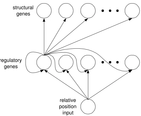
In the DRGN model, a genetic system is defined as a network ofN interacting
nodes (see Figure 1). The activation state of each node is a continuous variable
in the range [0,1], where 0 represented a completely inactive gene and 1 a fully
expressed gene. The network is updated synchronously in discrete time steps,
where each step represents the duration between cell divisions.
The network containsNsstructural nodes,Nrregulatory nodes and a single
input node. The structural nodes represent a subset of genes whose pattern of
activation specifies the current state of differentiation of the cell. These nodes
have no regulatory outputs, that is, their level of expression has no influence
on the future dynamics of the network. The regulatory nodes in the network
represent genes that play a regulatory role only.
The sharp distinction between structural and regulatory roles for genes
re-flects the traditional definition of a gene as the region of DNA encoding a single
protein [1]. Proteins are typically classed as either structural or regulatory and
genes have traditionally been classified according to the type of protein they
encode. It is now understood that the regulation of gene expression is a
signifi-cantly more complicated process than initially thought [28]. Genes may code for
multiple products via alternative splicing, and regulation may occur at stages
respect therefore, our model represents a first approximation to the complexity
of the regulatory process, with the potential for future refinement.
The input node was used to specify the relative position of the cell in the
lineage. After division, this node was set to 0 in the left daughter and 1 in
the right daughter. This minimal external input reflects the combined effects
of the different contextual signals received by the two cells resulting from their
respective positions in the embryo. A clear example of this type of signal is the
pop-1 gene inC. elegans, which is differentially expressed in the two daughters
produced following an anterior–posterior cell division [25]. It is important to
note that, at the level of abstraction of the DRGN model, this input does not
need to be assigned any single biological function. Rather than explicitly
requir-ing that cell fate be specified by any particular mechanism (such as asymmetric
division or inductive signals), it simply indicates that there is some difference
in regulatory context between the two daughter cells.
In most organisms, the time-scale for a single cell division is measured in
minutes or hours [1]. The time taken for an individual transcription event is
generally shorter, therefore a single cell cycle may consist of multiple
tion events. To capture the potential complexity of the interacting
transcrip-tion factors, we have used a network in which the regulatory nodes are fully
connected. Thus an individual link in the network does not necessarily
repre-sent a direct physical interaction, but rather the degree of influence that the
transcription of the source gene at timethas on the transcription of the target
gene at time t+ 1, where each time step represents a single cell division that
may entail multiple transcription events.
These interactions can be summarised in a weight matrix, in which the entry
at rowi, columnjspecifies the influence that genejhas on genei. These entries
may be positive or negative, depending on whether the product produced by
genej is an activator or a repressor in the regulatory context of genei. A zero
of self-connections (i.e. from nodeito nodei) allows for the possibility of genes
influencing their own regulation.
The state of the network was updated synchronously, with the activation of
nodeiat timet+ 1,ai(t+ 1), given by
ai(t+ 1) =σ¡ωiI(t) +
Nr
X
j=1
wijaj(t)−θi¢ (1)
whereNr is the number of regulatory nodes,ωi is the level of interaction from
the single input,I, to nodei,wij is the level of the interaction from node j to
nodei,θi is the activation threshold of nodei, andσ(.) is the sigmoid function,
given by
σ(x) = 1
1 +e−x (2)
4.2
The Developmental Process
The set of nodes and links of a DRGN represent the set of genes and their
interactions in a model organism. To simulate the developmental process of the
organism, the network was used to generate a cell lineage in the following way.
The original network, representing a fertilised egg cell, was initialised by setting
all node activations to 0 and the relative position input to 0.5. The activation
of each gene was then updated once. Cell division was implemented by creating
two copies of the network with identical weights and node activations. The
relative position input was set to 0 in the left daughter and 1 in the right
daughter, representing the different contextual signals received by each cell as
a consequence of its position in the embryo. The state of the network was
again updated and a new division occurred. This process was repeated until the
4.3
The Evolutionary Process
To derive a suitable set of gene interactions for performing the cell lineage tasks,
an automated machine learning technique was used to find a set of weights for
each network. An evolutionary algorithm (EA) was selected as an appropriate
search technique based on prior experience, the distributed nature of the
repre-sentation being evolved and its extensibility for a variety of tasks and parameter
settings. Note that, although EAs are inspired by evolutionary processes in
bi-ology, the intention in this study is not to model the evolution ofC. elegans per
se. Other automated learning techniques could also have been applied.
A simple evolutionary search strategy called the 1+1 ES was used [2].
Ini-tially a single network was generated with uniformly distributed random weights
in the range [−1,1]. The error values for this individual were calculated as
de-scribed below and stored. A new network was derived from this network by
adding uniformly distributed random values in the range [−0.5,0.5] to a
ran-domly chosen subset of the network weights (typically 10%). The error values
for the modified individual were calculated and compared to that of the original
individual. The individual with the lowest error was retained and used as the
basis for the creation of a further new network. This process was repeated for a
specified number of generations, or until a satisfactory solution was discovered
(described in Section 5).
Two related error values were calculated for each target cell, measuring the
difference between the pattern of activation of its structural nodes and the
pat-tern of activation of the corresponding cell in the target lineage. One error value
was based on the number of incorrect gene activations, the other incorporated
a measure of the degree of incorrectness.
The first error value, theNumber of Gene Errors (NGE)measured the
num-ber of incorrect structural gene activations in a cell. A correct gene activation
than or equal to 0.5 if the target activation was 0. The NGE was calculated by
N GE=
C X j=1 Ns X i=1 φ(pji, f
j
i) (3)
where C is the number of terminal cells in the lineage, Ns is the number of
genes in each target pattern,pji is the activation of geneiin the target pattern
jandfij is the activation of the structural geneiin the network corresponding
to cellj and φ(.) is given by
φ(pji, fij) =
0 if¡
(pji = 1)∧(f j i >0.5)
¢
∨¡
(pji = 0)∧(f j i ≤0.5)
¢
1 otherwise.
(4)
The NGE was used in the first and third tasks to halt evolution when a “perfect”
solution (no remaining incorrect gene activations) was found.
The second measure, the Sum Squared Error (SSE), measured the
differ-ence between the target activation (either 1 or 0) and the continuous-valued
activation of each node. The SSE was calculated by
SSE= C X j=1 Ns X i=1
(pji −f j i)
2
(5)
The SSE was used as the basis for comparing two networks during evolution.
5
Cell Lineage Tasks
5.1
Task A: Initial Cell Diversification
5.1.1 Aim
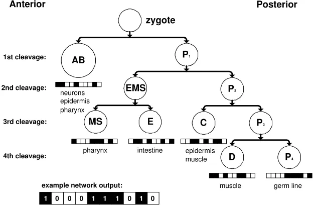
The initial cell divisions of C. elegans are invariant, with each precursor cell
dividing to produce a somatic cell, which goes on to form part of the body of
the embryo, and a further precursor cell. After the fourth division, the precursor
cell forms the basis of the organism’s germ line [38] (see Figure 2). The aim of the
of a well-characterised biological developmental sequence, and investigate its
behavior by requiring it to generate a diverse set of expression patterns.
5.1.2 Task Description
The first task involved generating a cell lineage corresponding to the initial
diversification of six founder cells inC. elegans embryogenesis, from which the
remaining cells will develop.
InC. elegans (and many other organisms) there is not a clear relationship
between the initial branches of the cell lineage and terminal cell fate. While
the intestine and germ cells are all derived from the E and P4cells respectively, epidermal cells are derived from both the AB and C cells. Conversely, the
daughters of the AB cell will eventually differentiate into neuronal, epidermal
and muscle cells [36]. Therefore, no strong correlations between the cells
pro-duced during initial diversification can necessarily be assumed. For this reason,
we defined six random patterns of structural gene activation corresponding to
the six cells at the beginning of each simulation trial (see Figure 2). The use of
random patterns represents the lower limit of task correlation where each target
developmental lineage is essentially arbitrary. Performance on a more correlated
target was evaluated in Task B (see Section 5.2).
5.1.3 Method
In Task A, a lineage was developed until six cells corresponding to the AB, MS,
E, C, D and P4cells had been generated. The patterns of activation of the Ns
structural genes in each of these cells were then compared to the corresponding
target pattern and the NGE and SSE calculated.
In order to explore the relationship between the task complexity and level of
regulation required, a family of parameterised networks were generated, varying
the size of the target pattern of each terminal cell (Ns= 4, 8, 12, 16, 20) and the
combination, 10 sets of target patterns and 10 initial networks were randomly
generated. A set of target patterns was generated by initialising the target
pattern of activation of each of the six cells such that each gene had a 50%
chance of being on or off. Each network was tested against each target pattern
(i.e. a total of 100 trials for each combination). Each trial was run for up to
50,000 generations, halting earlier if a solution with an NGE of zero was found.
For the purpose of comparison, a family of parameterised Boolean networks
were also generated, varying the number of regulatory nodes (Nr = 4, 8, 16)
and the level of connectivity (K = 2, 4, 6). These networks were evolved to
match the same sets of target patterns as the DRGN model. In the case of the
Boolean networks, the relative position input was incorporated by adding an
additional node to theNrregulatory nodes that could have regulatory outputs
to other nodes, but no regulatory inputs. Similarly, Ns additional structural
nodes were added that could have inputs from the regulatory nodes, but no
outputs. A cell lineage was generated from the network using the same process
as the DRGN (described in Section 4.2). The EA used to search for suitable
networks was the same as that used for the DRGN (described in Section 4.3),
except that, at each step, a new network was created using two steps. First,
each regulatory interaction had was randomly rewired with probability 0.05.
Second, the output of each of the Boolean updating rules for a given node was
flipped with probability 0.05.
5.1.4 Results
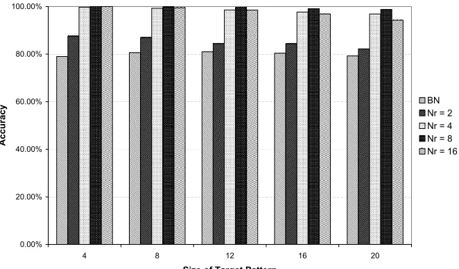
The DRGNs demonstrated competence on the cell diversification task, with
the majority of trials evolving a solution with greater than 90% accuracy (see
Figure 5a). The best performance on all sizes was shown by networks with
eight regulatory nodes (100% for 4-bit targets to 98.7% for 20-bit targets). The
networks with four and sixteen regulatory nodes achieved a similar level of
considerably lower, suggesting that some minimum level of regulatory
complex-ity was required to in order to perform the differentiation task. Interestingly,
there appeared to be an “optimal” level of regulation. The networks with eight
regulatory nodes consistently achieved higher levels of accuracy than those with
sixteen regulatory nodes within the range of target patterns used in this study.
A possible explanation is that this level of regulation represents a balance in the
trade off between the complexity of the task and the complexity of the search
space, which increases with the number of regulatory nodes. Furthermore, the
length of time required for evolution to find a good network with eight regulatory
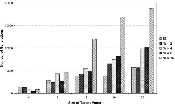
nodes scaled more slowly as the size of the task increased (see Figure 5b).
While the performance of the network with two regulatory nodes was
sig-nificantly less accurate, considering the size of the more complex tasks and the
minimal input provided, the performance (over 80% accuracy) was still
surpris-ingly good: twenty structural genes in each of six target patterns equates to a
total of 120 bits of output, generated from only a single bit of input provided
for each of five divisions. Clearly a significant amount of information can be
stored by the regulatory interactions within a DRGN.
Only the results of the best performing set of Boolean networks (N = 16; K =
2) are shown (see Figure 5a). As can be clearly seen, all of the DRGNs (including
those with two regulatory nodes) outperformed the Boolean networks. Closer
investigation of the Boolean network solutions revealed that they were generally
unable to make sufficient use of the input bit to differentiate their subsequent
patterns of activation. The errors generally occurred when two sister cells (e.g. E
and MS) remained on the same trajectory and hence displayed identical patterns
of activation.
To provide insights into the space of possible DRGNs that the EA is
search-ing, we calculated both the average performance of each individual network
across the ten target patterns as well as the average performance on a
pattern tended to find solutions with similar levels of residual error, suggesting
that good solutions could be reached by the EA from any part of the space.
How-ever, a greater level of variation was observed between the average residual error
for different target pattern sets. Variation across the pattern sets indicates that
some sets of patterns are consistently more difficult than others for the class of
DRGNs. A likely cause is that the “easier” target pattern sets contain a higher
degree of systematic structure, with fewer inconsistent interactions.
5.2
Task B: Combinatorial Control of Cell Lineages
5.2.1 Aim
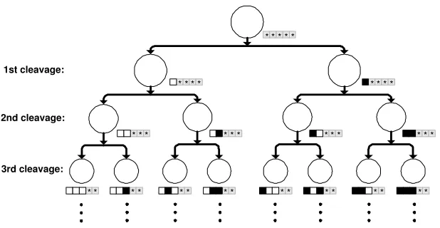
A common feature of eukaryotic cell lineages is the use of combinatorial gene
expression to allow a relatively large number of individual cell fates to be
spec-ified by a much smaller number of regulatory genes [1] (see Figure 3). In C.
elegans, it has been proposed that specific genes may act as a binary switch
to control the diversification of cell fates of a series of divisions [20]. The aim
of the second task was to explore the ability of the DRGN model to generate
complex, correlated developmental trajectories using combinatorial activation
of a limited number of genes.
5.2.2 Task Description
After each cell division, the network was required to distinguish between the two
newly created cells by the deactivation of a structural gene in the left daughter,
and the activation of the corresponding structural gene in the right daughter.
The target patterns of gene activation after the first division therefore, were
“OFF” in the first gene of the left daughter and “ON” in the first gene of
the right daughter. After the second division, “OFF–OFF” in the leftmost
daughter, followed by “OFF–ON”, “ON–OFF”, and finally “ON–ON” in the
a solution capable of generating a single cell lineage to a great depth at the
expense of all other lineages, a requirement was imposed to correctly match the
target patterns of activation in all cells at a given level before the next level was
generated (i.e. the two cells at the first level had to be correctly specified before
the four cells at the second level were generated, and so on).
5.2.3 Method
The network structure, error measures and EA were used as described in
Sec-tion 4. Again, the effect of different levels of regulaSec-tion was explored by the use
of a parameterised family of networks in which the size of the regulatory layer
was varied (Nr = 2, 4, 8, 16). Ten trials, each initialised with a random set
of network weights, were run for each value of Nr. As the target pattern was
open-ended (arbitrarily large cell lineages could potentially be generated), each
trial has halted when there had been no further improvement in SSE for 50,000
generations.
5.2.4 Results
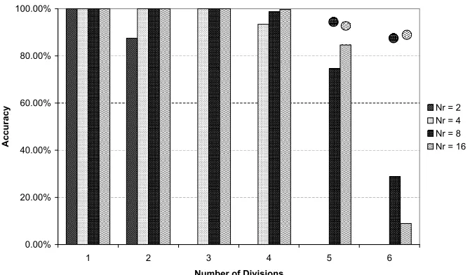
The largest combinatorial cell lineages were, unsurprisingly, generated by the
networks with eight and sixteen regulatory nodes (see Figure 6). For each of
these regulatory layer sizes, the EA managed to find at least one solution capable
of generating the first five levels of cell division (32 terminal cells) with 100%
accuracy and the sixth level of cell division (64 terminal cells) with 87% accuracy
(on average, 335 correct gene activations out of a total of 384 genes). Again,
the benefit of increasing the size of the regulatory layer appeared to diminish
beyond eight regulatory nodes.
Task B was in several respects a more difficult problem than Task A. Whereas
fitness in the first task was measured solely on the basis of the end products of
the differentiation process (the terminal cells), in the second task each of the
in its trajectory. Task B was also more difficult due to the greater depth of
the lineage and the increased density of the expression patterns. The pattern
of each cell differed from that of its sibling by only one bit, resulting in many
parts of the lineage tree having very similar expression patterns.
5.3
Task C: Termination of Cell Lineages
5.3.1 Aim
The final simulation task aimed to further investigate the ability of DRGNs to
control temporal sequences of information and provide correct output signals at
appropriate points in time. At a certain point in development, differentiation
of a particular cell lineage is complete, and division ceases. The timing of this
event is also under genetic control. One of the best understood examples of
genes controlling developmental timing inC. elegans is the interaction between
thelin-4 andlin-14 genes. These two genes control the timing of cell division
events in multiple cell types. Mutations to these genes result in phenotypes in
which specific stages of larval development are either skipped or repeated. The
temporal pattern of larval development is controlled by the level of expression
oflin-14, which decreases over time due to repression brought about by
increas-ing levels of lin-4 activation. Other interactions of this type have since been
discovered (for a review, see [30]).
5.3.2 Task Description
The final developmental task required the evolution of a network that was able
to specify the appropriate terminal point of each lineage beyond which cells
stopped dividing. As targets, we used several of the sublineages2 taken from
cell lineage ofC. elegans [36] (see Figure 4). Each of these sublineages forms a
branch of the lineage tree of initial cell divisions shown in Figure 2. One of the
structural genes was designated to have control over the the termination of cell
division, such that a cell divided so long as this gene was active, but stopped
dividing once this gene became inactive. As in Task B, the network was required
to match the correct decisions of all cells at a given level before the next level
was generated.
5.3.3 Method
The network structure, error measures and EA were used as described in
Sec-tion 4. Four different target lineages corresponding to the sublineages of cells
D (39 terminal cells), E (39 terminal cells), C (95 terminal cells) and MS (187
terminal cells) were used. The effect of varying the level of regulation was
ex-plored by varying the size of the regulatory layer (Nr = 2, 4, 8, 16). For each
combination of target lineage andNr, 10 trials were run, each initialised with a
random set of network weights. Each trial was run for 250,000 generations, or
until a solution with an NGE of zero was found.
5.3.4 Results
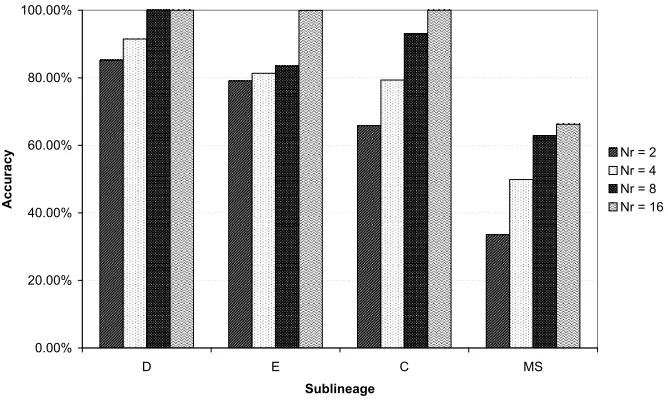
DRGNs were evolved that were able to generate sublineages D, E, and C with
100% accuracy and the MS sublineage with 66.2% accuracy (see Figure 7). The
performance on each of the sublineages is discussed in order of increasing size.
Sublineage D: For each regulatory layer size, the EA was able to find a
perfect solution in at least one of the ten trials and all ten of the trials involving
networks with eight and sixteen regulatory genes found a perfect solution.
Sublineage E: Perfect solutions were found by the EA in all ten of the trials
involving networks with sixteen regulatory nodes but only two of the trials
D and E both had the same number of terminal cells (39), the asymmetrical
arrangement of the left and right branches of sublineage E rendered it a more
difficult task. For sublineage D, the network was not required to make any
symmetry breaking decision until the third division. For sublineage E, this
de-cision was not only required one division earlier, but the subsequent trajectories
were mutually exclusive, increasing the information needing to be stored in the
regulatory interactions.
Sublineage C: The EA found perfect solutions in all but one of the trials
involving networks with sixteen regulatory nodes, and in six of the ten trials
involving networks with eight regulatory nodes.
Sublineage MS: The MS sublineage proved considerably more difficult than
the other sublineages. The greatest accuracy (66.2%) was obtained by a DRGN
with sixteen regulatory nodes. As well as being more than twice as large as
the previous sublineage, the MS sublineage also had a more irregular structure.
The MS sublineage consists of two major branches (MSa and MSp) that are
highly similar in many respects (as in sublineage C), however, there are two
critical differences. The right branch contains a lineage that undergoes apoptosis
(programmed cell death) after five divisions—a division earlier than the point at
which the corresponding lineage on the left branch terminates. This irregularity
posed a problem for the DRGNs as they were essentially being required to
learn to recognise a single special case out of 32 otherwise regular lineages.
Similarly, the left branch contained a single lineage that terminated after eight
divisions, where the corresponding lineage in the right branch terminated after
seven divisions, representing a single special case out of the 28 otherwise regular
lineages that had not yet terminated at that point. The exact cause of these
types of irregularities in the real C. elegans cell lineages varies on a case by
interaction between cells generated along the midline of the embryo [36]. The
failure of DRGNs at this point suggests a possible case where a more information
rich description of a cell’s spatial position or other physical factors may be
required.
6
Discussion and Conclusion
The results reported in this paper demonstrate that a network of interacting
genes is able to control the developmental trajectories of a moderate number of
individual cells with only a minimal level of external input. Networks with less
than ten regulatory genes were consistently able to control the activity patterns
of up to twice as many structural genes on tasks involving target patterns that
were random (Task A), correlated (Task B) or consisted of complex symmetrical
and asymmetrical lineages (Task C). The only information provided to the
net-work in each case was its relative position in the lineage after division—whether
it lay on the left or the right (anterior or posterior).
The first task, matching specified target patterns, showed that generating
arbitrary patterns of coordinated behaviour is relatively easy for DRGNs.
Fur-thermore, a trade was observed between the complexity of the task, represented
by the size of the target patterns, and the size of search space, determined by
the number of regulatory nodes in a network. This balance challenges the
intu-ition that larger problems are necessarily going to be solved more efficiently by
a larger network.
The second task, involving the generation of unique patterns for each level
of a cell lineage in a combinatorial fashion, demonstrated the ability of DRGNs
to maintain and transmit information over a number of division cycles. It also
highlighted a possible limitation of the EA used to find the network weights.
Theoretically, a network with N structural genes should be able to represent
limits performance, but rather the ability of the EA to find a suitable means
of representing the trajectories. Examining the final evolved networks revealed
that they tended to use most of their state space to represent the early
divi-sions. While this resulted in very robust performance on the initial divisions,
later divisions required the state space to be partitioned into increasingly small
compartments, and errors became more frequent.
The third task, matching the lineage topologies of severalC. elegans
sublin-eages, demonstrated the ability of the DRGNs to store temporal information.
Examining the state space trajectories representing each lineage revealed that
the network exploited gradients of activity to control the timing of division
ter-mination. This final task also demonstrated that not all lineage topologies were
equally easy to generate and that their difficulty was not necessarily correlated
with the size of the lineage. It was significantly easier to find a network able to
generate sublineage D than sublineage E, despite the fact that both contained 39
cells. The irregularity of sublineage E, with respect to its self similarity across
different scales, proved to be more challenging for the networks. This insight was
supported by further tests in which cell lineages were generated from random
networks—a significant portion of the lineages contained self similar patterns,
whereas none contained the type of asymmetric pattern observed in sublineage
E.
The competence of the network performance suggests that the DRGN model
is sufficient, given the definition of our developmental tasks, to simulate
biolog-ically inspired behaviours up to a reasonable level of complexity. The failures
of the networks are also instructive, indicating a potential role for other
infor-mational signals in the control of embryonic development. The simplicity of the
DRGN model makes it amenable to the use of machine learning techniques to
find networks able to generate specific patterns of behaviour. Furthermore, this
simplicity enables analysis of the found networks, providing some insight into
The innate tendency of control mechanisms based on recurrent networks to
generate systematic or quasi-systematic structures may offer some insight into
the topologies of cell lineages observed in nature. If the control of one particular
lineage topology is more easily generated than another, it is possible that the
patterns of development exhibited by biological organisms may reflect
inher-ent biases in their gene network controllers. The fact that some of these self
similar structures are broken, not by innate control of termination, but rather
by apoptosis, suggests both a means for evolution to circumvent these innate
control tendencies and also a possible explanation for some instances of
apop-tosis. It is not always clear why particular cell lineages are formed at all if the
resulting cell is only going to be killed at some later point in development [26].
One answer may be that it is easier to internally program the development of
a systematic lineage topology and utilise additional signals to “prune” excess
branches. Incorporating the additional mechanisms required to explore this
hy-pothesis represent one of the potential extensions that could be applied to the
DRGN model.
The design of the DRGN model and its assessment using a variety of cell
lineage tasks provide a window into the complexity of the control tasks solved by
every multicellular organism as it develops from a single cell to an embryo. It is
axiomatic that development involves the control of gene expression in both time
and space, and simulation forces the computational aspects of these processes
to be explicitly incorporated into models. In particular, simulating cell lineage
control with the DRGN model enabled us to explore the influence of network
architectures on the shape of developmental lineages. Observed cell lineage
topologies may reflect inherent biases of the developmental processes that
con-struct them, which are in turn constrained by the fundamental properties of the
Acknowledgments
An early version of this paper appeared in the proceedings of ACAL 2003 [14]
and we thank H. Abbass, the conference reviewers and two anonymous reviewers
of this paper for their comments. We also thank R. Azevedo, J. Hallinan, J.
Mattick, U. Platzer, B. Tonkes and members of the Complex and Intelligent
Systems group for useful discussions and comments. This study was supported
by an APA to NG and an ARC grant to JW.
References
1. Alberts, B., Bray, D., Lewis, J., Raff, M., Roberts, K., & Watson, J. D.
(1994). Molecular Biology of the Cell, 3rd ed. New York, NY: Garland.
2. B¨ack, T., Fogel, D., & Michalewicz, Z. (1997). Handbook of Evolutionary
Computation. Oxford, UK: Oxford University Press.
3. P. J. Bentley (Ed.). (1999). Creative Evolutionary Design. San Francisco,
CA: Morgan Kaufman.
4. Bodnar, J. W. (1997). Programming the Drosophila embryo. Journal of
Theoretical Biology,188, 391–445.
5. Bongard, J. & Pfeifer, R. (2003). Evolving complete agents using artificial
ontogeny. In F. Hara & R. Pfeifer (Eds.), Morpho-functional Machines:
The New Species (Designing Embodied Intelligence) (pp. 237–258). Berlin:
Springer-Verlag.
6. Braun, V., Azevedo, R. B. R., Gumbel, M., Agapow, P.-M., Leroi, A. M. &
Meinzer, H.-P. (2003). ALES: cell lineage analysis and mapping of
7. Davidson, E. H., McClay, D. R., & Hood, L. (2003). Regulatory gene
networks and the properties of the developmental process. Proceedings of
the National Academy of Science of the USA,100, 1475–1480.
8. de Jong, H. (2002). Modeling and simulation of genetic regulatory systems:
A literature review. Journal of Computational Biology,9, 67–103.
9. Di Paolo, E. A., Noble, J., & Bullock, S. (2000). Simulation models as
opaque thought experiments. In M. Bedau, J. McCaskill, N. Packard, &
S. Rasmussen (Eds.), Artificial Life VII (pp. 497–506). Cambridge, MA:
The MIT Press/Bradford Books.
10. Eggenberger, P. (2003). Genome-physics interaction as a new concept to
re-duce the number of genetic parameters in artificial evolution. In R. Sarker,
R. Reynolds, H. Abbass, K.-C. Tan, R. McKay, D. Essam, & T. Gedeon
(Eds.), Proceedings of the IEEE 2003 Congress on Evolutionary
Computa-tion(pp. 191–198). Piscataway, NJ: IEEE Press.
11. Elman, J. L. (1990). Finding structure in time. Cognitive Science, 14,
179–211.
12. Fleischer, K. (1996). Investigations with a multicellular developmental
model. In C. G. Langton & T. Shimohara (Eds.), Artificial Life V (pp.
229–236). Cambridge, MA: The MIT Press/Bradford Books.
13. Furusawa, C. & Kaneko, K. (2000). Complex organisation in multicellularity
as a necessity in evolution. Artificial Life,6, 265–281.
14. Geard, N. & Wiles, N. (2003). A gene regulatory network for cell
differ-entiation inCaenorhabditis elegans. In H. Abbass & J. Wiles, Proceedings
of the Australian Conference on Artificial Life (ACAL 2003) (pp. 86–100)
15. Hasty, J., McMillen, D., Isaacs, F., & Collins, J. J. (2001). Computational
studies of gene regulatory networks: in numero molecular biology. Nature
Reviews Genetics,2, 268–279.
16. Hogeweg, P. (2000). Shapes in the shadow: Evolutionary dynamics of
morphogenesis. Artificial Life, 6, 85–101.
17. Hornby, G. S., Lipson, H., & Pollack, J. B. (2003). Generative
representa-tions for the automated design of modular physical robots. IEEE
Transac-tions on Robotics and Automation,19, 703–719.
18. Huang, S. & Ingber, D. E. (2000). Shape-dependent control of cell growth,
differentiation, and apoptosis: Switching between attractors in cell
regula-tory networks. Experimental Cell Research,261, 91–103.
19. Jan, N. J. & Jan, L. Y. (1998). Asymmetric cell division. Nature, 392,
775–778.
20. Kaletta, T., Schnabel, H. & Schnabel, R. (1997). Binary specification of
the embryonic lineage inCaenorhabditis elegans. Nature,390, 294–298.
21. Kauffman, S. A. (1993). The Origins of Order: Self-Organization and
Selection in Evolution. Oxford, UK: Oxford University Press.
22. Kitano, H., Hamahashi, S., & Luke, S. (1998). The perfect C. elegans
project: An initial report. Artificial Life,4, 141–156.
23. Kumar, S. & Bentley, P. (2003). Biologically inspired evolutionary design.
In A. M. Tyrrell, P. C. Haddow, & J. Torresen (Eds.), Proceedings of the
International Conference on Evolvable Systems 2003 (pp. 57–68). Berlin:
Springer.
24. Labouesse, M. & Mango, S. E. (1999). Patterning theC. elegansembryo.
25. Lin, R., Hill, R. J., & Priess, J. R. (1998). POP-1 and anterior-posterior
fate decisions in C. elegans embryos. Cell,92, 229–239.
26. Metzstein, M. M., Stanfield, G. M. & Horvitz, H. R. (1998). Genetics of
programmed cell death in C. elegans: past, present and future. Trends in
Genetics, 14, 410–416.
27. Mjolsness, E., Sharp, D. H., & Reinitz, J. (1991). A connectionist model of
development. Journal of Theoretical Biology,152, 429–453.
28. Orphanides, G. & Reinberg, D. (2002). A unified theory of gene expression.
Cell,108, 439–451.
29. Rose, L. S. & Kemphues, K. J. (1998). Early patterning of theC. elegans
embryo. Annual Review of Genetics,32, 521–545.
30. Rougvie, A. E. (2001). Control of developmental timing in animals.Nature
Reviews Genetics,2, 690–701.
31. Schnabel, R., Hutter, H., Moerman, D. & Schnabel, H. (1997). Assessing
normal embryogenesis in Caenorhabditis elegans using a 4D microscope:
variability of development and regional specification. Developmental
Biol-ogy,184, 234–265.
32. Sipper, M. (2002). Machine Nature: The Coming Age of Bio-Inspired
Computing. New York, NY: McGraw Hill.
33. Sol´e, R. V., Salazar-Ciudad, I., & Garcia-Fern´andez, J. (2002).
Com-mon pattern formation, modularity and phase transitions in a gene network
model of morphogenesis. Physica A,305, 640–654.
34. Somogyi, R. & Sniegoski, C. A. (1996). Modelling the complexity of genetic
networks: Understanding multigenic and pleiotropic regulation.Complexity,
35. Stanley, K. O. & Miikkulainen, R. (2003). A taxonomy for artificial
em-bryogeny. Artificial Life, 9, 93–130.
36. Sulston, J. E., Schierenberg, E., White, J. G., & Thompson, J. N. (1983).
The embryonic cell lineage of the nematodeCaenorhabditis elegans.
Devel-opmental Biology,100, 64–119.
37. Vohradsk´y, J. (2001). Neural model of the genetic network. The Journal
of Biological Chemistry,276, 36168–36173.
38. Wolpert, L. (1998). The Principles of Development. Oxford, UK: Oxford
University Press.
39. Wuensche, A. (1998). Genomic regulation modeled as a network with basins
of attraction. In R. B. Altman, A. K. Dunker, L. Hunter, & T. E. Klein
(Eds.), Pacific Symposium on Biocomputing ’98 (pp. 89–102). Singapore:
structural genes
regulatory genes
[image:35.595.171.443.120.343.2]relative position input
Figure 1: The structure of the DRGN model. Gene regulation is modelled using
a partially connected network of N nodes. Section 4.1 describes the different
AB
EMS
MS E C
D P1
P2
P3
P4
zygote
neurons epidermis pharynx
pharynx intestine epidermis muscle
muscle germ line 1st cleavage:
4th cleavage: 3rd cleavage: 2nd cleavage:
Anterior Posterior
0
1 0 0 1 1 1 0 1 0
[image:36.595.149.467.211.416.2]example network output:
Figure 2: The cell lineage of very earlyC. elegans embryogenesis. Each
precur-sor cell cleavage results in the production of one somatic cell, which will divide to
generate epidermal, intestinal, neural and muscle cells, and a further precursor
cell. The final precursor cell, P4, gives rise to the germ line (redrawn from [36]).
Also shown is an example of the target activation patterns used in Task A, for
a trial with 10 structural genes. The enlarged example pattern illustrates the
correspondence between the patterns in the figure and the target activation of
1st cleavage:
3rd cleavage: 2nd cleavage:
* * * * *
* * * * * * * *
* * *
* * * * * * * * *
[image:37.595.152.461.261.421.2]* * * * * * * * * * * * * * * *
Figure 3: A cell lineage detailing the production of unique cell lineages by
combinatorial gene activation. The target patterns of gene activation used in
Task B are shown below each cell. The representation is the same as that shown
in Figure 2 except that greyed out squares represent genes whose output is not
E
l r l r
dv dv
D
d v d v
d v d v
ar pl ar pl
C
x
MS
d v d v
l r x
x
x x
x x
x x
x x
x x
x
Figure 4: The C. elegans sublineages used in Task C. All divisions occur
along the anterior–posterior axis unless otherwise specified as being along the
dorsal(d)–ventral(v) or left(l)–right(r) axes. An x indicates a cell that undergoes
apoptosis. The vertical axis of each lineage provides an indication of the
rela-tive timing of each division event, however, for the purposes of the simulations
reported here, all divisions at a given level occurred simultaneously. Redrawn
[image:38.595.135.476.169.478.2]Figure 5a: The DRGN performance on Task A. All results are averaged over
100 trials (10 random starting positions for each of 10 random sets of target
patterns). For comparison the accuracy of the best performing Boolean network
(withNr = 16 andK = 2) (BN) is also shown. Accuracy was defined by the
number of remaining incorrect structural genes (NGE) as a percentage of the
Figure 5b: The length of time taken by the EA in Task A before no further
Figure 6: The DRGN performance on Task B. The average accuracy of the
DRGNs is shown for each level of division, after there had been no improvement
for 50,000 generations. Each bar indicates the accuracy averaged across all ten
trials. Average accuracy after the second division forNr= 2 and after the fourth
division forNr= 4 was 0.00%. The circles indicate the accuracy averaged across
only those trials that actually reached that level of division (i.e. the trials in
which a network correctly specified only four levels of division were not included
Figure 7: The DRGN performance on Task C. The average accuracy achieved by
the DRGNs on each of the D, E, C and MS sublineages ofC. elegans, averaged